
Abstract
Two types of modeling and simulation as service configuration problems are formally defined and their complexities are analyzed. Optimization and heuristic solutions for these configuration problems are introduced. The important engineering parameters related to the schemes and their scalability are also investigated.
Keywords
1. Introduction
The modeling and simulation as a service (MSaaS) approach has been maturing for the past 3–4 years. It introduces many advantages for both military and civilian purposes.1–5 These advantages include but are not limited to on-demand self-service, broad network access, resource pooling, rapid elasticity, ease of technical administration, cost reduction, flexibility and fault tolerance.6–8 MSaaS also fits well to the recent trends in information technologies.
At the first glance, it is not easy to see the distinction between software as a service (SaaS)3,6,9–11 and MSaaS because MSaaS is in essence a special subset of SaaS. 2 The difference between MSaaS and SaaS becomes clearer when the service-oriented approach (SOA) and distributed simulation technologies are considered, because federating models or simulations into a composite MSaaS has special challenges and dynamics. Before elaborating on these special challenges, we first would like to clarify the term federation, which has a different meaning in cloud computing from modeling and simulation (M&S). In cloud computing, the term “federation” is used not only for federating software, but also for infrastructure or platforms, and therefore a federation may also mean a cloud service that integrates various resources in the form of infrastructure as a service (IaaS) (e.g., memory, processor time, etc.) from multiple datacenters.7,12 On the other hand, in the MSaaS domain, federations integrate multiple MSaaSs either in a standalone application or service module (SM; i.e., a service in service-oriented architecture approach) form, and are categorized into four broad classes, as shown in Table 1.
Types of modeling and simulation as service federations.
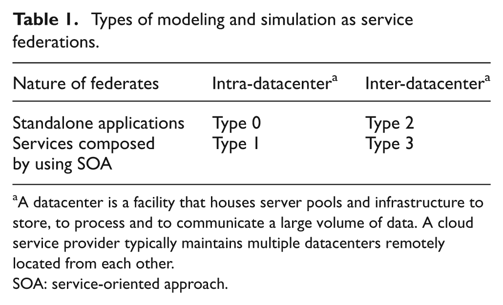
A datacenter is a facility that houses server pools and infrastructure to store, to process and to communicate a large volume of data. A cloud service provider typically maintains multiple datacenters remotely located from each other.
SOA: service-oriented approach.
Type 0: Multiple MSaaSs in the form of standalone applications located in the same datacenter are federated. 12
Type 1: Multiple SMs located in the same datacenter are composed into a composite MSaaS following SOA.
Type 2: Various software applications from various datacenters that may belong to different clouds are integrated into a seamless software federation by a MSaaS provider.
Type 3: Not complete software applications, but software modules and data located in multiple datacenters are brought together for dynamically configured service-oriented software federations. The datacenters that provide SMs may belong to different clouds (i.e., cloud service provider).
Let us clarify the difference between Type 2 and 3 by using a military MSaaS13,14 example depicted in Figure 1. Joint theater level simulation (JTLS), joint conflict and tactical simulation (JCATS) and virtual battle space (VBS2) are three widely used combat modeling software systems. 13 They work at different resolution levels. JTLS works in theater level to simulate scenarios with large units in very large areas. On the other hand, VBS2 is a very high resolution model that also provides three-dimensional visualization services for a relatively limited number of entities in a limited space. JCATS is in between these two models. JTLS, JCATS and VBS2 can be integrated into a Type 2 federation by using a runtime infrastructure (RTI) as defined in high-level architecture (HLA). 13 Please note that the co-location of JTLS and RTI in Figure 1 is just an example. Any of these federates can be co-located in a datacenter. Alternatively, services provided by RTI can be distributed in multiple datacenters.
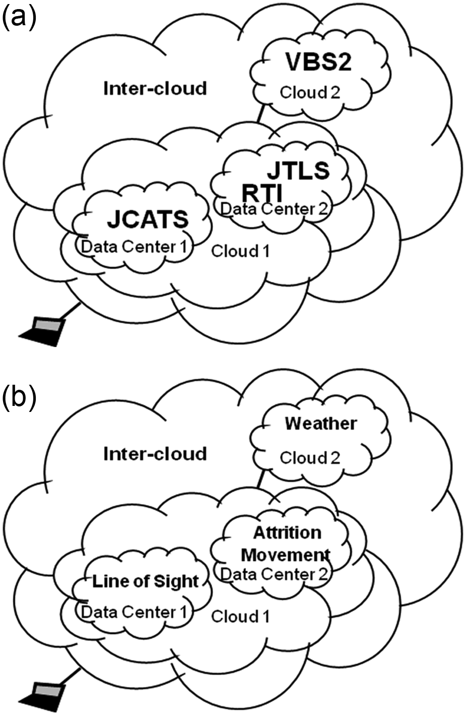
An example for (a) Type 2 and (b) Type 3 modeling and simulation as service inter-datacenter federations.
In Type 3, instead of complete combat models, software modules that models different aspects of theater are federated. In other words, services from multiple data centers are composed into a composite MSaaS. For example, a software module in one datacenter can make the line of sight calculations, and another one from another datacenter computes the effects of weather on the results. Configuring a Type 3 federation is definitely a more challenging task.
For the realization of a Type 2 or 3 inter-datacenter federation, the first task is the configuration of the federation, which is the selection of the services offered by datacenters to integrate for a given simulation task. When the federation is being configured, all the policy and physical constraints, performance expectations and interoperability requirements need to be satisfied. Among these, interoperability requirements 15 are a special challenge for MSaaS. In an inter-datacenter, there can be multiple MSaaSs that can provide the same service. Therefore, determining that the federates are interoperable with each other and selecting the set that fits best to the constraints and performance expectations is a new challenge. We call this challenge the MSaaS inter-datacenter federation (MIF) configuration (MIFC). In this paper, we define MIFC and introduce solutions for that.
In Section 2, the Type 2 MSaaS Inter-datacenter Federation Configuration (MIFC2) problem is formally defined. We also prove that MIFC2 is NP-complete and therefore introduce a heuristic algorithm for it. Section 3 is for Type 3 MSaaS Inter-datacenter Federation Configuration (MIFC3). MIFC3 is also a complex problem. However, for MIFC3, we follow a different approach and introduce an optimization algorithm based on exhaustive search in the solution space. We also define MIFC3 as a multi-criteria design problem with posterior articulation of user preferences. 16 MIFC3 is a new territory for federating models because it is based on SOA and service composition, and therefore it promises new opportunities and advancements in M&S. In Section 4, we give the results from our experiments where we also investigate how scalable the optimization algorithm for MIFC3 is. We conclude our paper in Section 5.
2. Type 2 modeling and simulation as a service inter-datacenter federation configuration
MIFC2 should support autonomous service and federation management, and has two phases in a federation execution: during startup, after startup. Starting a federation up takes time, because all federates need to connect to the federation and register/subscribe for the simulated objects. 13 MIFC2 configures the federation to minimize the startup time. After the startup, time performance of the federation (i.e., the fastest simulation speed that the federation can manage) is also important. Therefore, MIFC2 should reconfigure the federation to reach the desired simulation speed when requirements or constraints change.
2.1 Definition of the MIFC2 problem
The sequence of events when starting a HLA federation depends on federation agreement. However, the following events and sequence are typically a part of any HLA federation startup process:
RTI starts;
all federates start and join the federation;
all federates register the object classes that they will update during execution;
all federates update the initial status of their entities;
all federates subscribe for the object classes that they are interested in;
federates are updated about the initial status of the entities by RTI;
the federation starts moving forward.
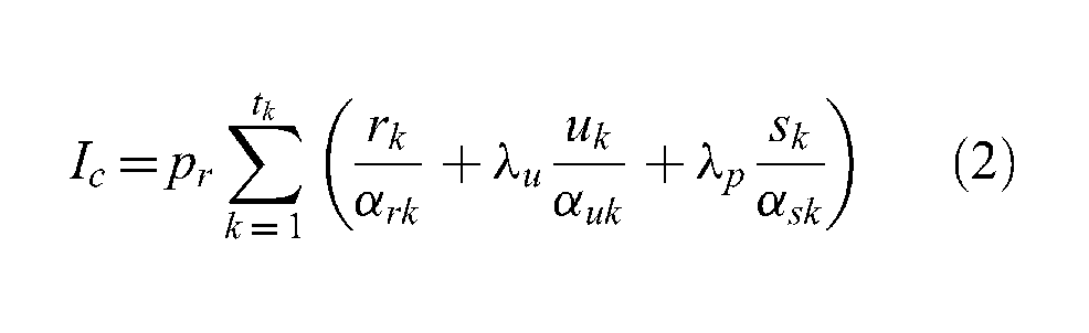
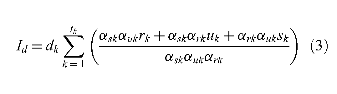
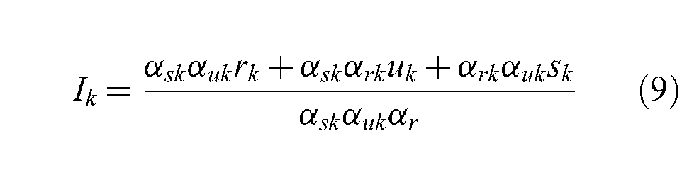
Therefore, the time required for starting up a federation, Is, is positively related to the propagation delay dk between every federate k and the RTI, the average processing time pr that the RTI needs for processing a registration message, the number of object classes rk that every federate k registers to the federation, the number of entities uk (i.e., the entities can be aggregated or atomic) for which every federate k publishes status updates during the startup of the federation, and the number of objects sk that every federate k subscribes from the federation. This relation is shown in Equation (1), where αrk, αuk and αsk are the encapsulation gain of federate k for registration (i.e., the number of entities that can be registered by a single message), updates and subscriptions, respectively, tk is the total number of federates, λ u is the ratio between the processing time cost of a single registration and an update message and λ p is the ratio between the processing time cost of a single registration and a subscription message:
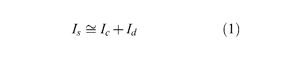
where processing delay Ic and propagation delay Id are
The MIFC2 objective function for startup is
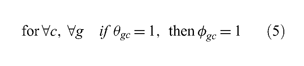
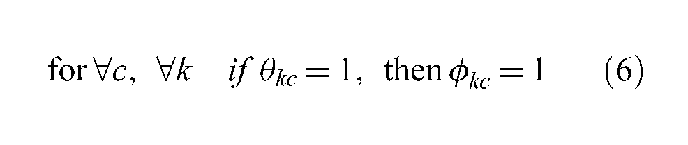
subject to
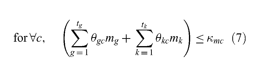
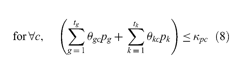
where
c is the id number for a datacenter;
g is the id number for a platform;
k is the id number for a federate (i.e., simulation software);
θgc = 1 if platform g is assigned to datacenter c;
ϕgc = 1 if platform g can be assigned to datacenter c;
θkc = 1 if federate k is assigned to datacenter c;
ϕkc = 1 if federate k can be assigned to datacenter c;
tg is the total number of platforms;
mg is the memory requirement for platform g;
mk is the memory requirement for federate k;
κmc is the total memory capacity available for the federation in datacenter c;
pg is the process time requirement for platform g;
pk is the process time requirement for federate k;
κpc is the total process time assigned for the federation by datacenter c.
Since bandwidth constraints are reflected into the propagation delay, which is taken into account within the objective function, we do not have a constraint about the communication links. Nevertheless, we assume that all the datacenters considered in our calculations are connected to each other. Therefore, we do not introduce an additional constraint for connectivity. Please also note that MIFC2 is assigning simulation applications to datacenters but not simulated entities to the applications. Therefore, the performance of each application in simulation tasks is not taken into account in our optimization.
If we assume that there are no constraints (i.e., we can assign all the federates and RTI to be run in a single datacenter), and neglect the propagation delay within a datacenter, the optimum solution for the federation startup is clearly when the entire federation is located in that datacenter but not distributed within the inter-cloud (i.e., the combination of clouds that include all the datacenters involved in running the federation). When any of Constraints 5–8 is applied, federates may need to be distributed to multiple datacenters within the inter-cloud, and therefore their initial locations (i.e., datacenter) must be selected carefully.
We can transform a 0-1 knapsack problem to an optimal MIFC2 problem in a polynomial time as follows. Stage 1: Map each item in the 0-1 knapsack problem to a federate for the optimal MIFC2 problem. Each federate has memory requirement mk equal to the weight wk of its related item in the 0-1 knapsack problem. Processing time requirement pk is 0 for every federate. Each federate has rk number of objects to register, which is equal to the value vk of its related item in the 0-1 knapsack problem. The number of entities to subscribe sk and update uk is the same for all federates and equal to 1. Stage 2: Create n datacenters. Each datacenter has the same memory κmc and processing time constraints κpc. Memory constraint κmc is equal to the weight constraint W given for the 0-1 knapsack problem, and the processing time constraint κpc is equal to 1. The number of datacenters n is the number of datacenters that can host all federates (i.e., there is a solution for the optimal MIFC2 problem or in other words there are multiple knapsacks and the number of knapsacks is equal to the number that can hold all the items). Stage 3: Assign 0 to the memory mg and the processing time pg requirements for the RTI. Stage 4: Initialize all the other parameters defined in Equations (2) and (3) as 1. When we run MIFC2 for this configuration, the set of federates located in the same datacenter as the one selected for the RTI is the set of items selected for the optimal 0-1 knapsack. This proves the theorem. □
Since the optimal MIFC2 problem is NP-complete, we designed Algorithm 1 for MIFC2. This algorithm reaches a feasible solution, which is the approximation of the optimal MIFC2 for a given topology.
Type 2 modeling and simulation as a service Inter-datacenter Federation Configuration heuristic for the federation startup.
2.2 MIFC2 scheme after the federation startup
After the startup, the constraints, the requirements and the performance parameters may change. MIFC2 can observe these changes and relocate the simulation software and platforms accordingly. Two options are considered as the relocation parameter: the startup time Is given by Equation (1) and the federation execution speed Ie given by Equation (11):
Equation (11) excludes parameters related to the object registration and subscription included in Equation (1). The federation execution speed mainly depends on the number of updates ukr from a federate k to the RTI, and the number of updates urk from the RTI to federate k. Please note that the encapsulation gain for the update message from federate k to the RTI αkr may be different from that of αrk from the RTI to federate k. Please also note that the number of updates affects the federation execution speed more when the federation is time managed. In Equation (11), we do not take the execution speed of individual federates into account because the performance of individual federates is not related to the performance of MIFC2, although they affect the performance of federations. Please also note that runtime communications are very complex and dependent on the nature of scenario events being executed at a time.
From these two options, we selected startup time Is as the parameter for relocation after federation startup, because Is includes Ie and the number of update messages are related to the number of registration/subscription messages. Moreover, Is is still an important parameter after startup because federations crash during the execution, and the recovery time from a crash depends on the federation startup time.
Therefore, we can still use the same objective function, constraints and heuristic for MIFC2 after startup. However, during execution there is a risk of hysteresis effect that should be avoided. When several configurations have a similar Is value, the configuration may be changed continuously and frequently if not managed properly. We call this effect as the hysteresis effect. To avoid hysteresis, we designed Algorithm 2 with two stages to reconfigure the federation after startup.
The algorithm for federation reconfiguration after the federation startup.
Conservation stage: as long as Constraints 5–8 are satisfied and the condition at Equation (12) holds, MIFC2 does not attempt to relocate federates or RTI:
where
er is the desired federation execution speed (i.e., simulation time speed / real time speed);
ti is the federation execution speed in the last interval;
tm is the federation execution speed in the interval m;
i is the number of execution speed sampling intervals.
Adaptation stage: when MIFC2 finds a new configuration that has a Is value δs better than the current configuration, it reconfigures the federation. δs is called the aggressiveness value. The smaller δs is, the more responsive MIFC2 becomes against the changes in constraints and parameters. We examine the effect of this factor in our experiments, and present the results in Section 4.
3. Type 3 modeling and simulation as a service inter-datacenter federation configuration
In the previous section, we defined MIFC2 and proved that MIFC2 is a NP-complete problem. In this section, we define the MIFC3 problem. We do not analyze the complexity of MIFC3 in this paper. However, it is clearly more complex than MIFC2. Still, we will approach MIFC3 differently from our approach for MIFC2, and attempt to develop a scheme that finds the optimum solution through exhaustive search. We will later analyze the scalability of this approach in Section 4. Please note that a similar heuristic to the one developed for MIFC2 can also be applied to MIFC3 and vice versa.
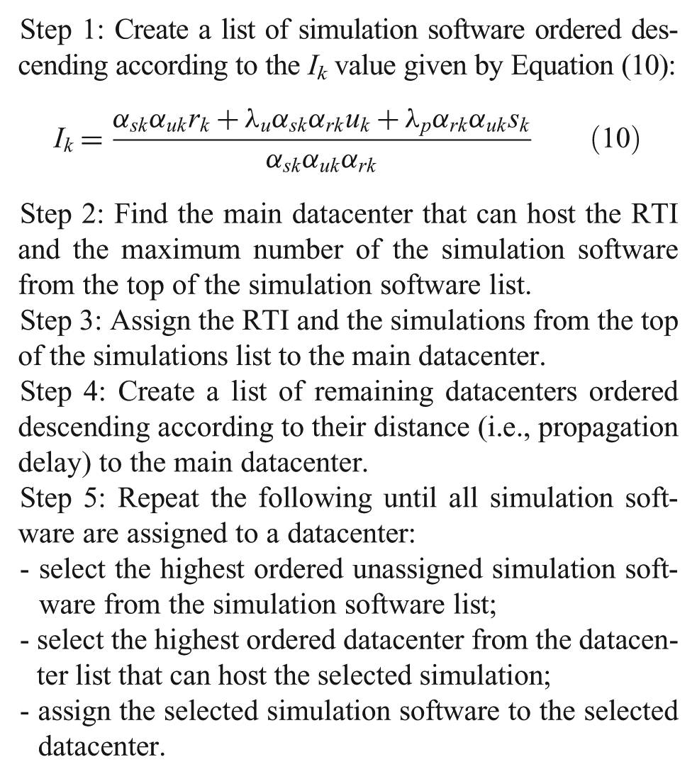
Main stages in Type 3 modeling and simulation as a service inter-datacenter federation configuration.
Before starting to explain MIFC3, we would like to clarify two terms: SM and service. An MIF consists of multiple SMs, such as geo SM, weather SM, etc. There may be multiple datacenters that can provide a service (i.e., MSaaS) that matches the requirements and constraints of a SM. Our scheme developed for MIFC3 first forms a set of all compatible services S = {s1,., sq} in the inter-cloud. Then, it creates a set of alternative MIF configurations A = {a1, …, ak}) composed of compatible services that fulfill the constraints of the application (i.e., ai = {sSM1, …, sSMn}, where n is the total number of SMs for the MIF). In the service selection process, our scheme takes also the policies of clouds into account. At the third stage, our MIFC3 scheme computes the criteria value for each of the alternative configurations in A and selects the non-dominated set of solutions (Ad⊆A) based on the criteria values. Finally, the non-dominated set of solutions Ad is given to the user for a posterior articulation of the user preferences.
3.1 The definition of MIFC3 problem
We use two criteria – cost c and performance p– when configuring a MIF. The cost c of a configuration is the total cost of all services that a MIF configuration consists of:
In Equation (13), ci is the cost of service i and n represent the number of services federated in the MIF, which is also equal to the number of SMs in the MIF. For the same service, clouds may apply multiple price policies such as on-demand, reserved and spot 3 with different quality of service (QoS) parameters. We treat a service with different prices as different services. For example, a cloud gives different on-demand and spot prices for the same geo-service. For us, those services are separate with different prices and QoS, although they are actually the same service.
In this paper, we relate the performance of an application to the average response time T and failure rate β in keeping the average response time promised by the cloud. An architecture and framework to measure and monitor average response time and failure rates are explained by Garg et al. 9 Average response time and failure rates 18 may be parametric values. For example, the time required for line of sight calculation may depend on the size of the terrain, which can change during federation execution. Service fan-out (i.e., the dependence of a service on some other for fulfillment) can also affect the response time. In our approach, we assume that an average value for the performance that takes also issues like fan-out into account can be given based on specified parameters and previous performance data. 9 Finally, performance can be treated as a generic criterion and related also to any other QoS or quality of experience (QoE) parameter. For example, propagation delay between the services and the application that federates the services is a very important parameter that impacts on the performance of a simulation federation. Without changing our MIFC3 scheme, average response time can be replaced with propagation delay when configuring a MIF. Moreover, our MIFC3 scheme allows using more than one criterion for performance if needed. In this paper, the performance criterion p is calculated as follows:
Please note that the number of datacenters, which provide services to a MIF, may be smaller than the number of services federated n, because one datacenter can provide more than one service for the MIF.
MIFC3 objectives are minimizing these criteria (i.e., c and p). Please note that our performance criteria p is a negative criterion, which means higher p implies an undesirable effect on the performance of the MIF. If a positive performance metric, such as sustainability or reliability, is selected, the objective becomes maximizing the performance criteria. For the criteria selected in this paper, MIFC3 objectives are minimize c; minimize p;
subject to
the datacenter that provides the MIF has a service-level agreement (SLA) to federate every service in the MIF; every service in the MIF is compatible with all the other services in the MIF; c ≤ ct; p ≤ pt;
where ct is the cost limit agreed with the user (SLA); pt is the performance limit agreed with the user (SLA).
This is clearly a multi-criteria design problem with posterior articulation of user preferences. Based on the nature of c and p, MIFC3 can also be treated as a multi-objective combinatorial optimization problem.
3.2 MIFC3 scheme
Our MIFC3 scheme can be divided into two main phases, the same as our MIFC2 scheme: the first phase is the proactive and distributed inter-cloud formation stage during which various data structures are created and maintained. In the second phase, a MIF that satisfies the requirements and constraints given by a user is formed.
1) Inter-cloud formation phase: for MIFC3 the following data structures need to be maintained by all the clouds that may provide MSaaS:
-compatibility strings set;
-service mapping matrix (SMM);
-service cost array (SCA);
-service performance array (SPA).
The first of these data structures is a set of compatibility strings S = {s1, s2, …, sq}. In S, each item si is represented as a binary string of length z, where z is the total number of services available in the inter-cloud. We call these binary strings compatibility strings. Each service has a fixed place in every compatibility string (i.e., a binary digit that represents a service is at the same location in every compatibility string). This fixed place of a service in a service compatibility string is also treated as the identification of the service.
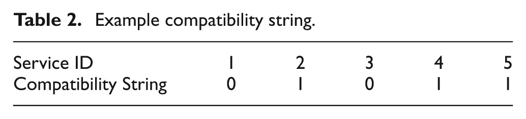
When a cloud makes a SLA for a service with another cloud, one bit is appended to all the compatibility strings in the compatibility strings set of the cloud. The appended bits to a compatibility string are set as “1” if all the other services indicated as “1” (i.e., compatible services) in the string are compatible with the new service, and as “0” otherwise. For example, in the compatibility string given in Table 2, Services 2, 4 and 5 are compatible with each other, which means that they can be federated in the same MIF. After this, a new string for each other service available in the inter-cloud and compatible with the new service is added into the set if there is not already another compatibility string that has both of these two services set as “1”. In these new strings only two services are set as “1” (i.e., the new service and the compatible service) and the others are set as “0”. If there is no service compatible with the new service, then a new string is added only with “1” for the new service and “0” for all the other services into the compatibility strings set.
Example compatibility string.
There may be multiple services available for the same SM in the inter-cloud. For example, there may be multiple datacenters that offer geo-services or the same service may be offered with various prices. Please remember our example to differentiate a SM from a service: a geo-service required for a MIF is a SM and the actual geo-service provided by a cloud is a service. A single service may also provide services for multiple SMs. For example, a service provided by a cloud can support both geo and weather SMs. Therefore, we need a data structure that maps SMs to services. We call this data structure the SMM. An example SMM is depicted in Table 3. Each SM is a row, and each service is a column in this matrix. If a service can support a SM, the related field is 1, and it is 0 otherwise. When a new service is registered to an inter-cloud, every cloud that has a SLA for this new service adds a new column to their SMM for the new service.
Example service mapping matrix.
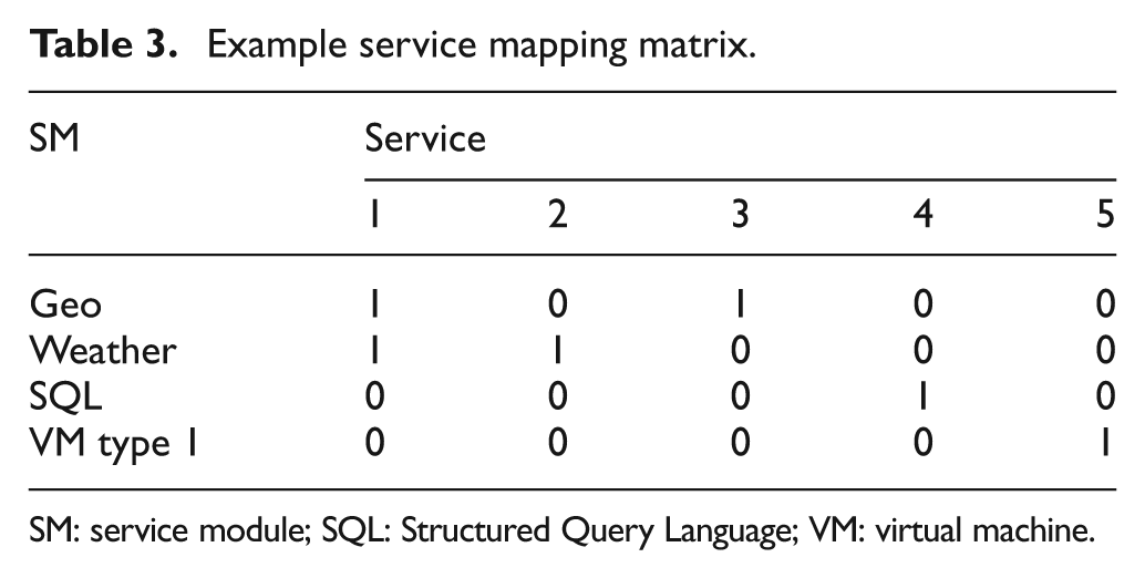
SM: service module; SQL: Structured Query Language; VM: virtual machine.
Each cloud also maintains the cost and the performance values for every service that they can federate in SCA and SPA, respectively.
2) MIF formation phase: MIF formation is illustrated in Algorithm 4. It starts when a cloud receives a request for a MIF. At the first step all the compatibility strings that include all the SMs in the requested MIF are derived from the compatibility strings set. For this the SM strings (i.e., the row for the SM in the SMM) for all SMs required for the MIF are multiplied (i.e., bitwise “and” operation) with each compatibility string one by one. If the result of the “and operation” is zero even for one SM string, the compatibility string is not included into the set of selected compatibility strings SMIF: SMIF⊆ S si∈SMIF iff si×SMMSM≠ 0 for ∀SM in the MIF
If SMIF is an empty set, it indicates that there is not a MIF configuration that can meet the requirements of the MIF. The user is informed that there is no feasible configuration and the process is terminated. If SMIF is not an empty set, Step 2 starts. For this, all the possible configurations for the compatibility strings in SMIF are listed. In each MIF configuration there is one and only one service selected for each SM. The resulted configurations are collected in alternative MIF configurations set A: A = {a1, a2, …, ak} ai = {sSM1, …, sSMn}
Then the cost c and the performance p values are calculated for all the alternative MIF configurations in A. If the cost c or performance p value of a configuration is above the limits (i.e., c > ct or p > pt), the configuration is removed from A. If A is empty at the end of this step, the user is informed that there is no feasible configuration and the process is terminated.
If A is not an empty set, there is at least one feasible configuration for the MIF request. If A includes only one configuration there is no need for the articulation of the preferences. The user is provided with the MIF according to the only MIF configuration in A. If there are multiple configurations in A, then all the configurations but the non-dominated ones are removed from A. In the non-dominated set there cannot be any configuration that has both cost c and performance p values larger than another configuration in the non-dominated set. The points linked with the bold line in Figure 2 are the non-dominated set for the example in the figure. If the non-dominated set includes only one configuration, there is no need for the articulation of the preferences. The user is provided with the MIF according to the only MIF configuration in the non-dominated set. If there are multiple configurations in the non-dominated set, the user selects the configuration for the MIF from the non-dominated set.
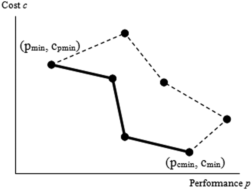
Non-dominated set example.
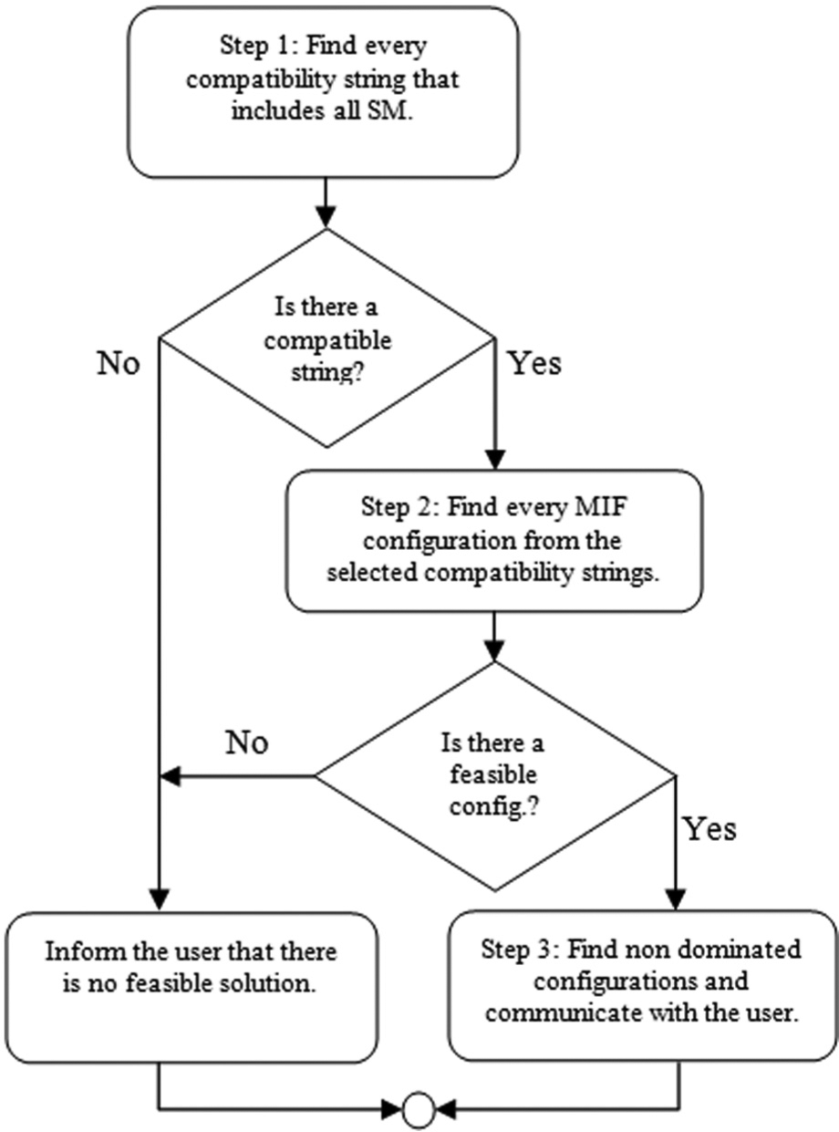
Main steps in the MIF formation stage.
4. Experimental results
We run experiments both for our MIFC2 and MIFC3 schemes. For MIFC2, we focused on the performance of the scheme, and tested its performance sensitivity against the changes in the number of datacenters, simulations and entities. For MIFC3, our focus is its scalability because it is not a heuristic but an optimization technique. We investigate up to how many SMs in a MIF and services in an inter-cloud our MIFC3 scheme can be feasible. For this we analyze parameters such as the expected number of compatibility strings investigated and configurations in the non-dominated solution sets.
4.1 Results from MIFC2 experiments
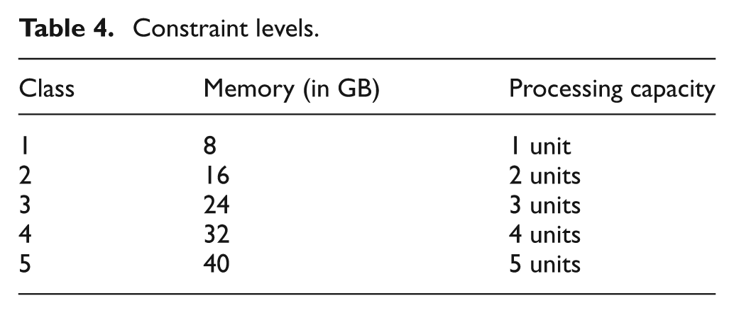
In this section we examine the performance of our MIFC2 heuristics through simulation, where a federation with one RTI and between 3 and 10 federates (i.e., a typical constructive simulation federation for a complex military M&S event 13 ) are run in an inter-cloud that has up to 10 datacenters. Each federate is assigned randomly between 1024 and 5120 entities. The memory and processing time requirements of federates are related to the number of entities that they simulate. The memory and processing time constraints of each datacenter are factored into five classes between one and five, as shown in Table 4. To study the sensitivity of the algorithms against the aggressiveness parameter δs, the simulation is run for five simulation days, and constraints of the datacenters are changed in time intervals distributed randomly according to exponential distribution with a mean value 6 hours.
Constraint levels.
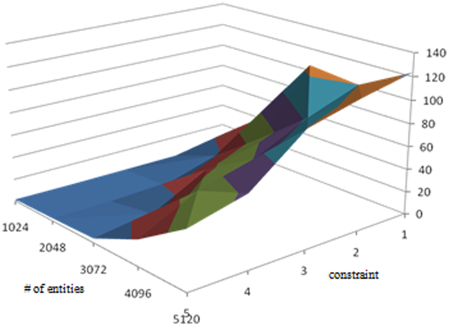
In Figure 3, the number of datacenters required to host the federation is depicted for various constraints and number of entity levels. This figure is important to better understand the other figures because the number of datacenters required to run a federation makes an impact on the performance of our MIFC2 scheme. When the constraint level is high, it means more resources are assigned to the federation by each datacenter. The processing time unit in Table 4 is the same unit as the one used for the federate processing time requirement. Therefore, when the constraint level is higher, the number of datacenters needed for a federation execution is less. On the other hand, when the requirements are higher, the number of datacenters involved for the federation execution also becomes higher.
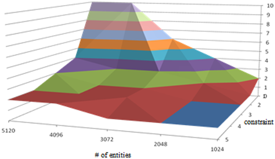
Number of datacenters involved in a federation execution.
The federation startup time is closely related to the number of datacenters over which the federation is distributed. The higher the number of datacenters, the higher the federation startup time becomes. Therefore, as the constraint level gets higher (i.e., the memory and process capacities allocated increase), the startup time decreases, as shown in Figures 4 and 5. The relation between the propagation delay (i.e., the average time required for transferring a packet from one datacenter to the other) and startup time is more trivial and is shown in Figure 5.
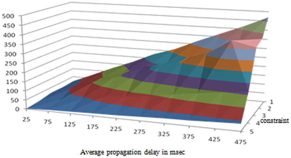
Average startup time in seconds.
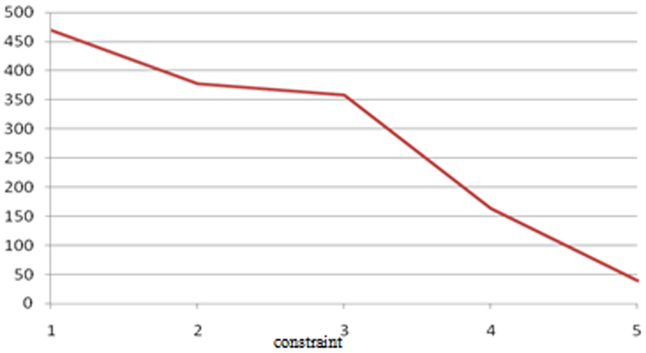
Average startup time in 100 ms for propagation delay 475 ms.
A similar relation also exists between the average number of entities simulated by the federates and the startup time. When federates have more entities to update, starting up a simulation takes longer. Figure 6 illustrates this relation when the propagation delay is 125 ms. For the other propagation delay values, the same relation is also observed.
Average startup time in seconds for propagation delay 125 ms.
In Figures 7 and 8, the sensitivity of the MIFC2 scheme against the aggressiveness parameter δs is illustrated when the propagation delay is 475 ms. We tested the algorithm for various aggressiveness factors, which is a percentage of the initial startup time for the federation. For shorter aggressiveness values (i.e., closer to 2%), the average startup time increases almost as long as the aggressiveness value comparing to the initial startup time. When the aggressiveness factor is higher (i.e., closer to 20%), the average startup time increases to less than 15% of the aggressiveness value compared to the initial startup time.
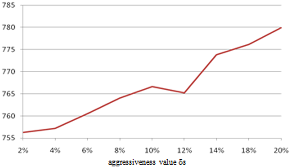
Average startup time in 100 ms for propagation delay 475 ms.
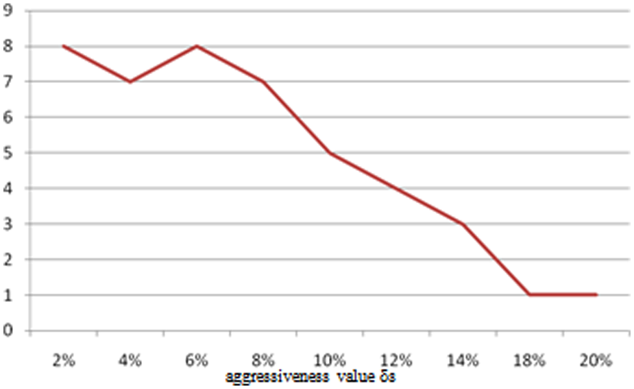
Number of configuration changes for propagation delay 475 ms.
As expected, the configuration is changed (i.e., the datacenters involved in the execution of the federation) less number of times when the aggressiveness value is higher. For example, when the aggressiveness value is 18% or 20%, the federation configuration changes only once on average during five days’ federation execution in our simulation set up.
4.2 Results from MIFC3 experiments
In our MIFC3 experiments we test with the following performance metrics:
α: the average number of compatibility strings in S;
ϕ: the average number of compatibility strings in SMIF;
δ: the average number of alternative configurations;
ε: the average number of non-dominated feasible alternative configurations.
These are important parameters because they imply the scalability of our scheme. For example, the number of alternative configurations gives the number of times that the cost and performance calculations are made and evaluated for reaching the non-dominated set. We tested these metrics against the factoring parameters given in Table 5. We assigned random values distributed according to the uniform distribution within the ranges in Table 5 to our factoring parameters, and observed the sensitivity of our performance metrics to the changes of those values.
Factoring parameters used in the experiments.
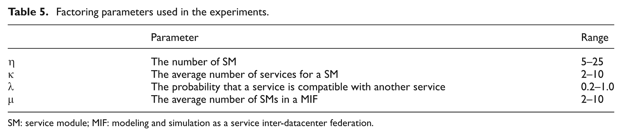
SM: service module; MIF: modeling and simulation as a service inter-datacenter federation.
The average number of compatibility strings for various numbers of available services (i.e., η×κ) and the compatibility probabilities (i.e., λ) are illustrated in Figure 9. Interestingly the number of compatibility strings is not correlated to the compatibility probability. As the number of services increases, the number of compatibility strings also increases, which is expected. The number of compatibility strings is slightly less than the number of services, which is negligible in terms of the amount of data for the memory and processing power requirements.
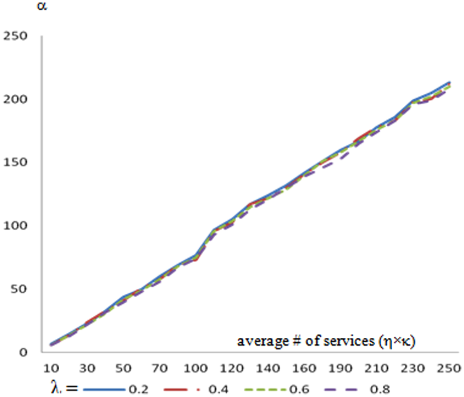
Average number of compatibility strings (α).
The average number of compatibility strings evaluated for a MIF is approximately one out of the tenth of the total number of compatibility strings when the compatibility probability is 0.4, as depicted in Figure 10. We observe that there is a linear relation between the number of compatibility strings and the number of services, which is again as expected. Nevertheless, we did not observe any relation between the number of compatibility strings (i.e., neither for the total number of compatibility strings α, nor for the number of compatibility strings selected for a MIF ϕ) and the compatibility probability λ.
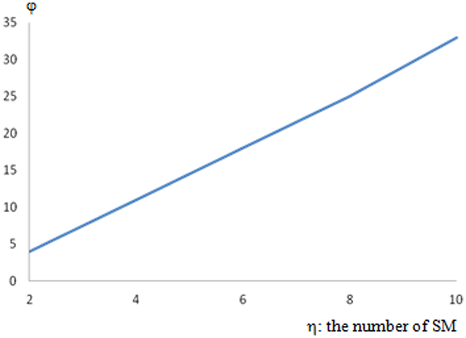
Average number of compatibility strings in SMIF for λ = 0.4.
When a MIF consists of 10 SMs, which have 10 services available on average, the average for the total number of alternative configurations δ is 330,000. This is a very reasonable number for such a demanding configuration. Even when the number of services available for each SM is 20 for 10 SMs, the total number of configurations is 5300. Therefore, we can run an exhaustive search for finding the optimum solution by using our MIFC3 scheme for a MIF that federates a high number of services. However, Figure 11 also implies that for a larger number of SMs the average number of alternative configurations becomes too many for an exhaustive search. Please note that the results in Figure 11 are for the compatibility ratio λ = 0.4.
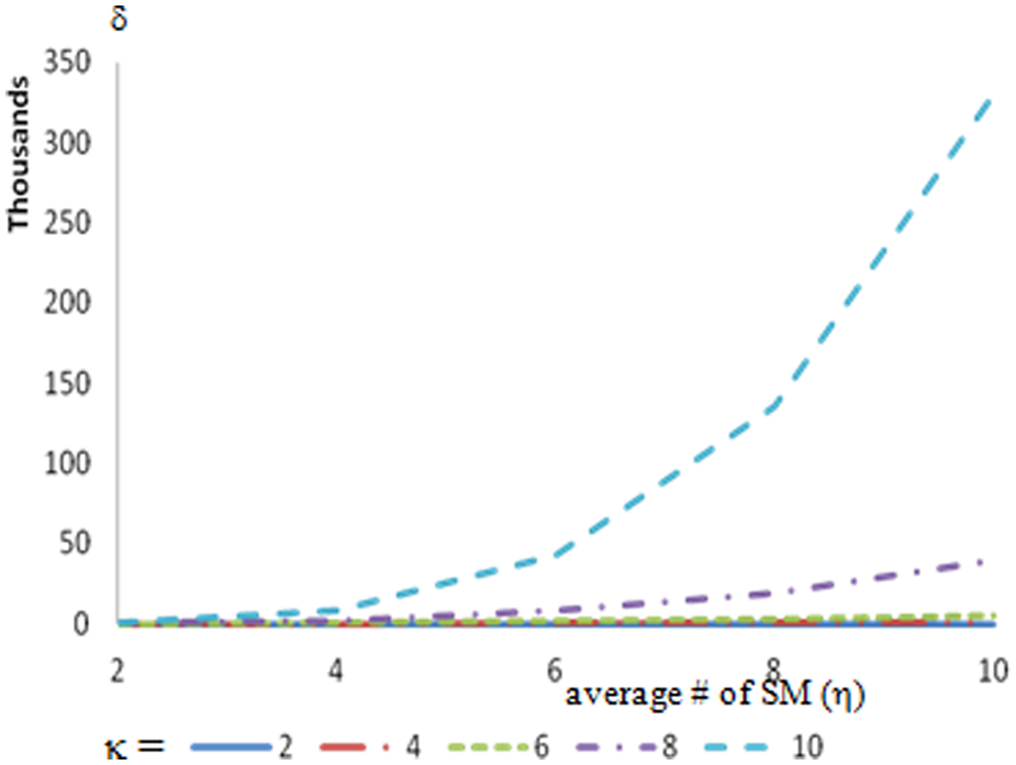
Average number of alternative configurations for a MIF when λ = 0.4.
The average number of alternative configurations in a non-dominated set is depicted in Figure 12. We did not apply any cost or performance limit criteria. Therefore, Figure 12 plots the upper bound, which is the worst case. Still the average number of configurations given to the user to select from is 8, which is very reasonable. Please note that the cost and performance values are assigned randomly to the services. When there is a correlation between cost and performance values the number of configurations in a non-dominated set becomes very small, often 1, which means that we end up with a single solution and there is no need for a posterior articulation of user preferences. Please also note that there is no correlation between the non-dominated set and the actual values assigned to cost and performance parameters. We did not observe any meaningful relation between the non-dominated set and the total number of alternative configurations either.
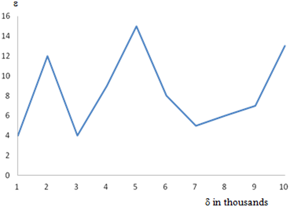
The average number of non-dominated alternative configurations ε.
5. Conclusion
Distributed simulations and inter-clouds introduce additional challenges for MSaaS, which make MSaaS a special subset of SaaS. In particular, interoperability requirements and the other constraints related to performance, resources and policies need to be taken into account when configuring a MSaaS federation in an inter-datacenter environment. A MIF can be one of four integration types. In Type 0 and 1, a single datacenter provides a MSaaS to the front end. In Type 2, multiple simulation systems (i.e., SaaS) from several datacenters are federated into a single MIF, which requires selection of the right set of standalone simulation applications that fulfill the requirements and the constraints. This configuration problem is called MIFC2 and is proven as NP-complete. MIFC3 is a more complex problem and selects the right SMs (i.e., models and functions) from the services available in multiple datacenters. For MIFC2 a heuristic is introduced. For MIFC3, an algorithm that finds the optimum solution is developed. A heuristic similar to our MIFC2 scheme can also be applied to the MIFC3 problem and vice versa.
Footnotes
Funding
This work was supported in part by EU FP7 Accountability for Cloud and Other Future Internet Services (A4Cloud) Project.