Use of the calibration approach in confidence intervals for mean response times of an open queueing network with feedback

Abstract

To construct various confidence intervals of mean response times for an open queueing network model with feedback, the calibration approach is used. In this paper, a data-based recurrence relation is used to compute a sequence of response times. Sample means from those response times are used to estimate true mean response times. With the help of numerical simulation study, we investigate the accuracy of the different calibrated confidence intervals of mean response times by calculating the coverage percentage and average length.

Keywords

Feedback calibration technique coverage percentage response time queueing network models

1. Introduction

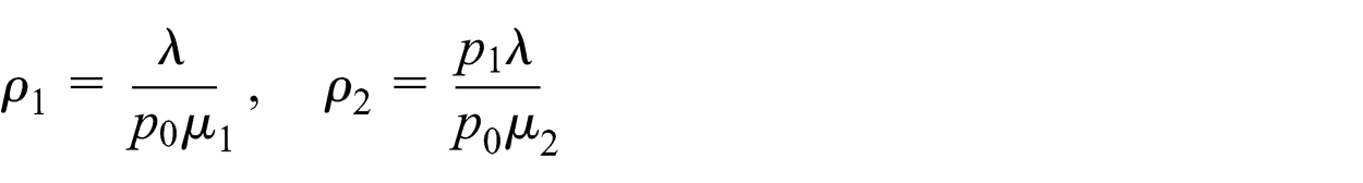
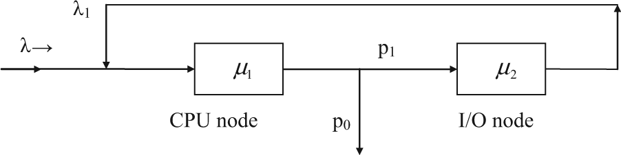
The response time is defined as the time spent by a customer from arrival until it departs. Consider a network model of a computer system with feedback in which a job may return to previously visited nodes. The system consists of a central processing unit (CPU) node and an input/output (I/O) node with respective service rates $μ_{1}$ and $μ_{2}$ . The external arrival rate is $λ$ . After service completion at the CPU node, the job proceeds to the I/O node with probability p ₁, and departs from the system with probability p ₀, where p ₀ = 1 –p _1. Jobs leaving the I/O node are always fed back to the CPU node (Figure 1). The successive service time at both nodes is assumed to be mutually independent and independent of the state of the system. The traffic intensity at the CPU node and I/O node is respectively given by

ρ_{1} = {\frac{λ}{p_{0} μ}}_{1}, ρ_{2} = {\frac{p_{1} λ}{p_{0} μ}}_{2}

Figure 1.

Two-stage open queueing network with feedback.

Intensity $ρ_{1}$ and $ρ_{2}$ can be interpreted as expected number of arrivals per mean service time. The condition for stability of the system is that both $ρ_{1}$ and $ρ_{2}$ are less than unity.

Statistical inference in queueing networks with feedback is rarely found in the literature and the work related in the past mainly concentrates on only parametric statistical inference, in which the distribution of population is with a known form. Basic properties of queueing networks are introduced by Disney.¹ Jackson’s theorem states that each node behaves like an independent queue.² Thiruvaiyaru et al.³ established that maximum likelihood estimators of the parameters of an open Jackson network are derived, and their joint asymptotic normality. Open queueing networks are useful in studying the behavior of computer communication networks.⁴

So far very few authors have studied the nonparametric statistical inferences. Efron^5–7 originally developed and proposed the bootstrap, which is a resampling technique that can be effectively applied to estimate the sampling distribution of any statistic. Gedam and Pathare^8–11 have studied the nonparametric statistical estimation approaches of various queueing network models. Chu and Ke¹² examined the statistical behavior of the mean response time for the M/G/1 queueing system using bootstrapping simulation. These same authors studied the interval estimation of mean response time for a G/M/1 queueing system using the empirical Laplace function approach.¹³ Chu and Ke also developed a data-based recurrence relation to compute a sequence of mean response times and constructed confidence intervals of mean response times for the G/G/1 queueing system using simulation.¹⁴

There is hardly any work regarding the use of the calibration technique in queueing networks with feedback. This motivates us to develop the nonparametric statistical inference of mean response time for a queueing network model with the feedback and use calibration technique to construct confidence intervals for mean response times $r_{1}$ and $r_{2}$ . The calibration technique is used for improving the coverage accuracy of any system of approximate confidence intervals. The idea of the bootstrap calibration technique is to first use bootstrap to estimate the true coverage of confidence intervals and the intervals are then adjusted by comparing with the target nominal level.

Nonparametric inference for estimating mean response time is discussed in Section 2 and the calibration technique is discussed in Section 3. In Sections 4–11 we have proposed different calibrated confidence intervals for mean response time. In Section 12, a numerical simulation study is conducted. All simulation results are shown by appropriate tables for illustrating performances of all estimation approaches. In Section 13 some conclusions are given.

2. Nonparametric estimation approach for mean response time

Let $(X_{i}, Y_{i}, i = 1, 2)$ be the nonnegative continuous random variables representing respectively inter-arrival times and service times of the CPU node and I/O node of a queueing network with feedback. The random variables $Y_{i}, i = 1, 2$ are independent of $X_{i}, i = 1, 2$ .

Let $(X_{1 j}, p_{0} Y_{1 j}, j = 1, 2 . . . . n)$ be a random sample drawn from $(X_{1}, Y_{1})$ that represents inter-arrival time and service time for the jth customer at the CPU node of a queueing network with feedback. Let $(p_{1} X_{2 j}, p_{0} Y_{2 j}, j = 1, 2 . . . . n)$ be a random sample drawn from $(X_{2}, Y_{2})$ that represents inter-arrival time and service time for the jth customer at the I/O node of a queueing network with feedback.

Let $R_{1 j}, j = 1, 2 . . . . n$ represent the response time of the jth customer at the CPU node of a queueing network with feedback, which is determined from $(X_{1 j}, p_{0} Y_{1 j}, j = 1, 2 . . . . n)$ . Similarly, $R_{2 j}, j = 1, 2 . . . . n$ represents the response time of the jth customer at the I/O node of a queueing network with feedback and is determined from $(p_{1} X_{2 j}, p_{0} Y_{2 j}, j = 1, 2 . . . . n)$ .

Let $W_{ij}, i = 1, 2 . j = 1, 2 . . . . n$ represent the waiting time of the jth customer at the ith node of a queueing network with feedback. Then

R_{ij} = W_{ij} + p_{0} Y_{ij}, i = 1, 2 . j = 1, 2 . . . . n

(1)

With the help of analysis by Kleinrock,⁴ we can evaluate $W_{ij}, i = 1, 2 . j = 1, 2 . . . . n$ the using recurrence relation given by

W_{1 j} = (R_{1, (j - 1)} + X_{1 j}) I ({R_{1, (j - 1)} > X_{1 j}})

(2)

W_{2 j} = (R_{2, (j - 1)} + p_{1} X_{2 j}) I ({R_{2, (j - 1)} > p_{1} X_{2 j}})

(3)

for $j = 2, 3 . . . . n$ and $W_{i 1} = 0, i = 1, 2$ , where $I (.)$ denotes the indicator function. Using Equation (1), we get

R_{1 j} = (R_{1, (j - 1)} + X_{1 j}) I ({R_{1, (j - 1)} > X_{1 j}}) + p_{0} Y_{1 j}

(4)

R_{2 j} = (R_{2, (j - 1)} + p_{1} X_{2 j}) I ({R_{2, (j - 1)} > p_{1} X_{2 j}}) + p_{0} Y_{2 j}

(5)

for $j = 2, 3 . . . . n$ and $R_{i 1} = Y_{i 1}, i = 1, 2$ . Equations (4) and (5) are the exact data-based recurrence relations for calculating response times $R_{ij}, i = 1, 2 . j = 1, 2 . . . . n$ that are exactly as a sequence of a customer’s response times for a queueing network with feedback, hence

{\hat{r}}_{i} = \frac{1}{n} \sum_{j = 1}^{n} R_{ij}, i = 1, 2

(6)

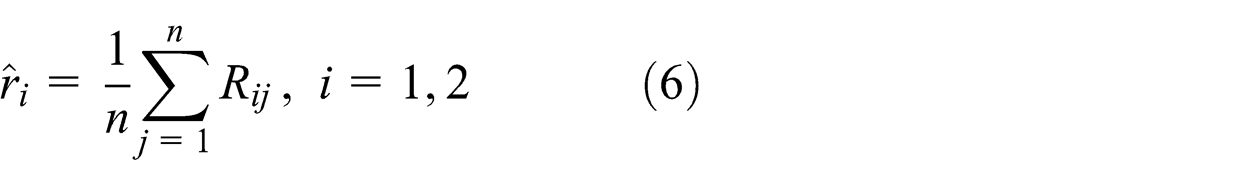
the arithmetic mean of these response times is a natural estimator of the mean response times $r_{i}$ , i = 1,2 for a queueing network with feedback.

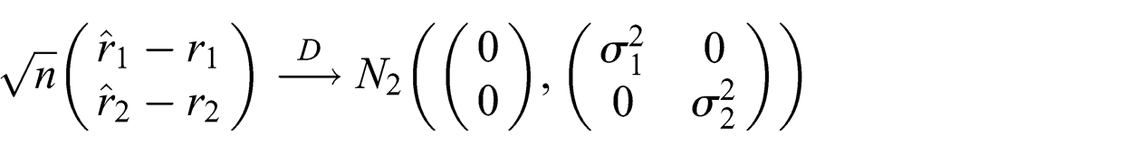
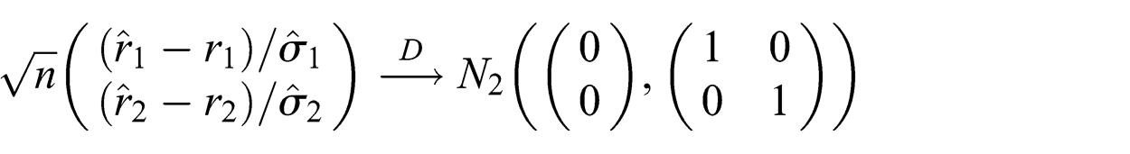
According to the Strong Law of Large Numbers,¹⁵ we know that ${\hat{r}}_{i}$ , i = 1,2 is a strongly consistent estimator of $r_{i}$ , i = 1,2. The true distributions of $(X_{i}, Y_{i}, i = 1, 2)$ are not often known in practice, so the exact distributions of ${\hat{r}}_{i}$ , i = 1,2 cannot be derived. However, under the assumption of $X_{i}$ and $Y_{i}$ being independent, the asymptotical distributions of ${\hat{r}}_{i}$ , i = 1,2 can be developed. By Slutsky’s theorem,¹⁶ we have

\sqrt{n} (\begin{matrix} {\hat{r}}_{1} - r_{1} \\ {\hat{r}}_{2} - r_{2} \end{matrix}) \overset{D}{\to} N_{2} ((\begin{matrix} 0 \\ 0 \end{matrix}), (\begin{matrix} σ_{1}^{2} & 0 \\ 0 & σ_{2}^{2} \end{matrix}))

where $σ_{i}^{2} = \frac{1}{n} \sum_{j = 1}^{n} (R_{ij} - {\hat{r}}_{i})^{2}, i = 1, 2$ , is the variance of $R_{ij}, i = 1, 2 . j = 1, 2 . . . . n$ and $\overset{D}{\to}$ denotes convergence in distribution. Then ${\hat{σ}}_{i}^{2}$ , $i = 1, 2$ is a strongly consistent estimator of $σ_{i}^{2}, i = 1, 2$ . Again applying Slutsky’s theorem, we have

\sqrt{n} (\begin{matrix} ({\hat{r}}_{1} - r_{1}) / {\hat{σ}}_{1} \\ ({\hat{r}}_{2} - r_{2}) / {\hat{σ}}_{2} \end{matrix}) \overset{D}{\to} N_{2} ((\begin{matrix} 0 \\ 0 \end{matrix}), (\begin{matrix} 1 & 0 \\ 0 & 1 \end{matrix}))

Thus, ${\hat{r}}_{i}$ , i = 1,2 is a strongly consistent and asymptotically normal (CAN) estimator with approximate variances ${\hat{σ}}_{i}^{2} / n, i = 1, 2 .$

3. Calibration technique

The actual coverage of a confidence interval procedure is rarely equal to the desired (nominal) coverage and often is substantially different. One way to think about the coverage accuracy of a confidence procedure is in terms of its calibration. We could construct a confidence procedure with exactly the desired coverage. Each calibration brings another order of accuracy but at a formidable computational cost. The calibration process produces a second-order accurate confidence point.¹⁷ As the calibration technique is used for improving the coverage accuracy of any system of approximate confidence intervals, we think that it is important to improve the accuracy of confidence intervals of mean response times in practical cases also. The bootstrap can be used to carry out the calibration.

The general theory of calibration is reviewed by Efron and Tibshirani,¹⁷ following the ideas of Loh,¹⁸ Beran,¹⁹ Hall²⁰ and Hall and Martin.²¹ The bootstrap calibration technique was introduced by Loh.^18,22 Let a confidence limit ${\hat{r}}_{i} [α]$ have probability $α$ of covering the true value $r_{i}$ , that is $P_{F i} {r_{i} \leq {\hat{r}}_{i} [α]} = α, i = 1, 2$ , where $F_{i}$ is unknown continuous probability distribution. For an approximate confidence limit there is true probability $β_{i}$ that $r_{i}$ is less than ${\hat{r}}_{i} [α]$ , say $β_{i} (α) = P_{F i} {r_{i} \leq {\hat{r}}_{i} [α]}$ . If we knew the function $β_{i} (α)$ then we could calibrate an approximate confidence interval to give exact coverage. Suppose we know that $β_{i} (0.06) = 0.05 and β_{i} (0.93) = 0.95$ . Then instead of $({\hat{r}}_{i} [0.05], {\hat{r}}_{i} [0.95])$ , we would use $({\hat{r}}_{i} [0.06], {\hat{r}}_{i} [0.93])$ to get a central 90% interval with correct coverage probabilities.

In practice we usually do not know the calibration function $β_{i} (α)$ . However, we can use the bootstrap to estimate $β_{i} (α)$ . The bootstrap estimate of $β_{i} (α)$ is $\overset{\land}{β_{i}} (α) = P_{\overset{\land}{F} i} {{\hat{r}}_{i} \leq {\hat{r}}_{i} {[α]}^{*}}$ , where $\overset{\land}{F_{i}}$ and ${\hat{r}}_{i}$ are fixed, while ${\hat{r}}_{i} {[α]}^{*}$ is the αth confidence limit based on the bootstrap dataset from $\overset{\land}{F_{i}}$ . The estimate $\overset{\land}{β_{i}} (α)$ is obtained by taking B bootstrap datasets and seeing what proportion of them have ${\hat{r}}_{i} \leq {\hat{r}}_{i} [α]^{*}$ .

4. Consistent and asymptotically normal calibrated confidence interval and normal calibrated confidence intervals for mean response time

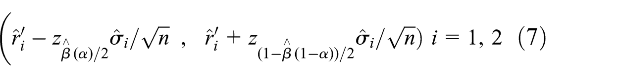
Using CAN estimators ${\hat{r}}_{i}$ , i = 1,2 and their associated approximate variances ${\hat{σ}}_{i}^{2} / n$ , i = 1,2, we construct calibrated confidence intervals for $r_{i}$ , i = 1,2. Let $z_{α}$ be the upper αth quantile of the standard normal distribution. Compute $\overset{\land}{β} (α) = P {r_{i} \leq ({\hat{r}}_{i} - z_{α / 2} {\hat{σ}}_{i} / \sqrt{n})}$ and $\overset{\land}{β} (1 - α) = P {r_{i} \leq ({\hat{r}}_{i} + z_{α / 2} {\overset{\land}{σ}}_{i} / \sqrt{n})}$ . Then approximately $100 (1 - α) %$ calibrated confidence intervals for $r_{i}$ , i = 1,2 are given by

{\hat{r}}_{i}' - z_{\overset{\land}{β} (α) / 2} {\hat{σ}}_{i} / \sqrt{n}, {\hat{r}}_{i}' + z_{(1 - \overset{\land}{β} (1 - α)) / 2} {\hat{σ}}_{i} / \sqrt{n}) i = 1, 2

(7)

For a sufficiently large value of n, the CAN calibrated confidence intervals approaches to normal calibrated confidence intervals.

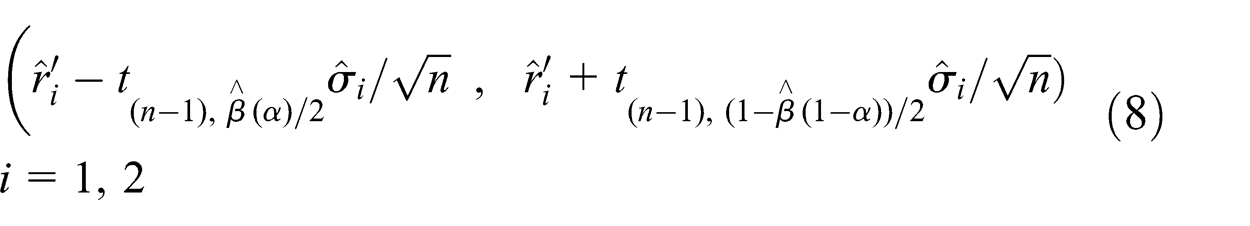
5. Student’s t calibrated confidence intervals (exact-t)

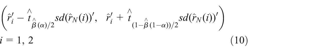
Let $t_{α}$ be the upper αth quantile of the Student’s t-distribution. Compute $\overset{\land}{β} (α) = P {r_{i} \leq ({\hat{r}}_{i} - t_{(n - 1), α / 2} {\hat{σ}}_{i} / \sqrt{n}}$ and $\overset{\land}{β} (1 - α) = P {r_{i} \leq ({\hat{r}}_{i} + t_{(n - 1), α / 2} {\hat{σ}}_{i} / \sqrt{n}}$ . Then the $100 (1 - α) %$ Student’s t calibrated confidence intervals for $r_{i}$ , i = 1,2 are given as

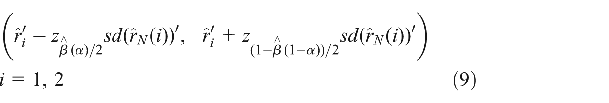
({\hat{r}}_{i}' - t_{(n - 1), \overset{\land}{β} (α) / 2} {\overset{\land}{σ}}_{i}' / \sqrt{n}, {\hat{r}}_{i}' + t_{(n - 1), (1 - \overset{\land}{β} (1 - α)) / 2} {\overset{\land}{σ}}_{i}' / \sqrt{n}) i = 1, 2

(8)

6. Standard bootstrap calibrated confidence intervals

According to the bootstrap procedure, a simple random sample $(X_{1 j}^{*}, p_{0} Y_{1 j}^{*}, j = 1, 2, . . . . n)$ and $(p_{1} X_{2 j}^{*}, p_{0} Y_{2 j}^{*}, j = 1, 2, . . . . n)$ called a bootstrap sample is taken from the empirical distribution function of $(X_{1 j}, p_{0} Y_{1 j}, j = 1, 2, . . . . n)$ and $(p_{1} X_{2 j}, p_{0} Y_{2 j}, j = 1, 2, . . . . n)$ , respectively. Using Equations (4) and (5), we can obtain $r_{ij}, i = 1, 2 . j = 1, 2, . . . . n$ as a sequence of customer’s response time. Similarly we can obtain $r_{ij}^{*}, i = 1, 2 . j = 1, 2, . . . . n$ . It follows that ${\hat{r}}_{i} = \frac{1}{n} \sum_{j = 1}^{n} r_{ij}, i = 1, 2$ is a natural estimate of the mean response time $r_{i}$ , i = 1,2 for a queueing network. ${\hat{r}}_{i}^{*} = \frac{1}{n} \sum_{j = 1}^{n} r_{ij}^{*}, i = 1, 2$ is called the bootstrap estimate of ${\hat{r}}_{i}, i = 1, 2$ . The above resampling process can be repeated N times. The N bootstrap estimates ${\hat{r}}_{i 1}^{*}, {\hat{r}}_{i 2}^{*}, \dots, {\hat{r}}_{iN}^{*}, i = 1, 2$ can be computed from the bootstrap resample. Averaging the N bootstrap estimates, we get that ${\hat{r}}_{N} (i) = \frac{1}{N} \sum_{j = 1}^{N} {\hat{r}}_{ij}^{*}, i = 1, 2$ is the bootstrap estimate of $r_{i}$ , i = 1,2 and the standard deviation of ${\hat{r}}_{i}$ , $i = 1, 2$ can be estimated by $sd ({\hat{r}}_{N} (i)) = {\frac{1}{N - 1} \sum_{j = 1}^{N} {({\hat{r}}_{ij}^{*} - {\hat{r}}_{N} (i))}^{2}}^{1 / 2}, i = 1, 2$ . By central limit theorem, the distribution of ${\hat{r}}_{i}, i = 1, 2$ is approximately normal. After computing $\overset{\land}{β} (α) = P {r_{i} \leq ({\hat{r}}_{i} - z_{α / 2} sd ({\hat{r}}_{N} (i)))}$ and $\overset{\land}{β} (1 - α) = P {r_{i} \leq ({\hat{r}}_{i} - z_{α / 2} sd ({\hat{r}}_{N} (i)))}$ we get $100 (1 - α) %$ standard bootstrap (SB) calibrated confidence intervals for $r_{i}$ , i = 1,2 as

\begin{matrix} ({\hat{r}}_{i}' - z_{\overset{\land}{β} (α) / 2} sd ({\hat{r}}_{N} (i))', {\hat{r}}_{i}' + z_{(1 - \overset{\land}{β} (1 - α)) / 2} sd ({\hat{r}}_{N} (i))') \\ i = 1, 2 \end{matrix}

(9)

7. Bootstrap-t calibrated confidence intervals

Considering N bootstrap estimates ${\hat{r}}_{i 1}^{*}, {\hat{r}}_{i 2}^{*}, \dots, {\hat{r}}_{iN}^{*}, i = 1, 2$ computed from the bootstrap resample, we compute $Z_{ij}^{*} = \frac{({\hat{r}}_{ij}^{*} - {\hat{r}}_{N} (i))}{sd ({\hat{r}}_{N} (i))}, i = 1, 2, j = 1, 2 . . . . N$ . Further $Z_{i 1}^{*}, Z_{i 2}^{*}, \dots, Z_{iN}^{*}, i = 1, 2$ follows an approximate t-distribution. Also compute $\overset{\land}{β} (α) = P {r_{i} \leq ({\hat{r}}_{i} - t_{α / 2} sd ({\hat{r}}_{N} (i)))}$ and $\overset{\land}{β} (1 - α) = P {r_{i} \leq ({\hat{r}}_{i} + t_{α / 2} sd ({\hat{r}}_{N} (i)))}$ . Then we get $100 (1 - α) %$ bootstrap-t calibrated confidence intervals for $r_{i}$ , i = 1,2 as

\begin{matrix} ({\hat{r}}_{i}' - {\overset{\land}{t}}_{\overset{\land}{β} (α) / 2} sd ({\hat{r}}_{N} (i))', {\hat{r}}_{i}' + {\overset{\land}{t}}_{(1 - \overset{\land}{β} (1 - α)) / 2} sd ({\hat{r}}_{N} (i))') \\ i = 1, 2 \end{matrix}

(10)

where ${\hat{t}}_{\hat{β} (α) / 2} and {\hat{t}}_{(1 - \hat{β} (1 - α)) / 2}$ equals the $α / 2$ percentile of the random sample $Z_{i 1}^{*}, Z_{i 2}^{*}, \dots, Z_{iN}^{*}, i = 1, 2$ .

8. Variance-stabilized bootstrap-t calibrated confidence intervals

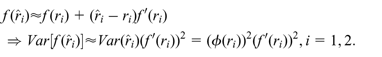
Let ${\hat{r}}_{i}, i = 1, 2$ be a strongly CAN estimator with approximate variances ${\hat{σ}}_{i}^{2} / {\hat{σ}}_{i}^{2} n n, i = 1, 2$ . Let ${\hat{σ}}_{i} = ϕ ({\hat{r}}_{i})$ . We find a transformation $f ({\hat{r}}_{i})$ such that $Var (f ({\hat{r}}_{i})) \approx constant$ . By the first-order Taylor series expansion and taking expectations on both sides, we get

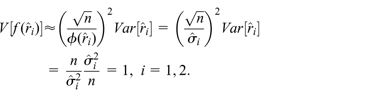
\begin{matrix} f ({\hat{r}}_{i}) \approx f (r_{i}) + ({\hat{r}}_{i} - r_{i}) f' (r_{i}) \\ \Rightarrow Var [f ({\hat{r}}_{i})] \approx Var ({\hat{r}}_{i}) {(f' (r_{i}))}^{2} = {(ϕ (r_{i}))}^{2} {(f' (r_{i}))}^{2}, i = 1, 2 . \end{matrix}

Now consider $f ({\hat{r}}_{i}) = \sqrt{n} \log (ϕ ({\hat{r}}_{i})), i = 1, 2$ is the variance-stabilizing transformation. Then we have

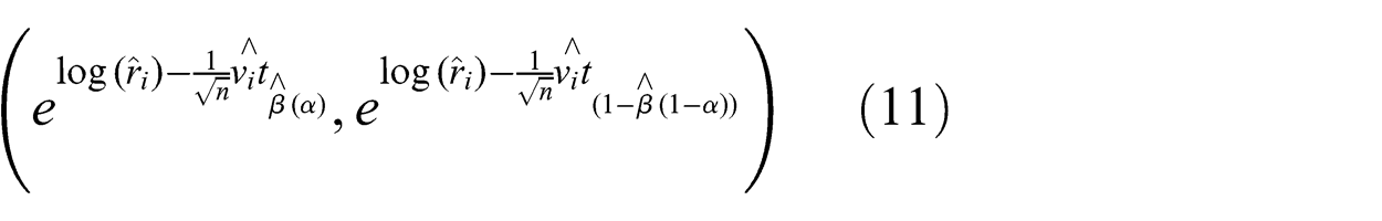
V [f ({\hat{r}}_{i})] \approx {(\frac{\sqrt{n}}{φ ({\hat{r}}_{i})})}^{2} V a r [{\hat{r}}_{i}] = {(\frac{\sqrt{n}}{{\hat{σ}}_{i}})}^{2} V a r [{\hat{r}}_{i}] = \frac{n}{{\hat{σ}}_{i}^{2}} \frac{{\hat{σ}}_{i}^{2}}{n} = 1, i = 1, 2 .

Here we consider N bootstrap estimates ${\hat{r}}_{i 1}^{*}, {\hat{r}}_{i 2}^{*}, \dots, {\hat{r}}_{iN}^{*}, i = 1, 2$ computed from the bootstrap resample. We calculate $θ_{ij}^{*} = \sqrt{n} \log ({\hat{r}}_{ij}^{*}) - \sqrt{n} \log ({\hat{r}}_{i}), i = 1, 2, j = 1, 2 . . . . N$ . Also compute $\overset{\land}{β} (α) = P {r_{i} \leq e^{\log ({\hat{r}}_{i}) - \frac{1}{\sqrt{n}} {\overset{\land}{v_{i} t}}_{1 - α / 2}}}$ and $\overset{\land}{β} (1 - α) = P {r_{i} \leq e^{\log ({\hat{r}}_{i}) - \frac{1}{\sqrt{n}} {\overset{\land}{v_{i} t}}_{α / 2}}}$ . Then we have $100 (1 - α) %$ variance-stabilized bootstrap-t (VST) calibrated confidence intervals for $r_{i}$ , i = 1,2 as

(e^{\log ({\hat{r}}_{i}) - \frac{1}{\sqrt{n}} {\overset{\land}{v_{i} t}}_{\overset{\land}{β} (α)}}, e^{\log ({\hat{r}}_{i}) - \frac{1}{\sqrt{n}} {\overset{\land}{v_{i} t}}_{(1 - \overset{\land}{β} (1 - α))}})

(11)

where ${\overset{\land}{v_{i} t}}_{\overset{\land}{β} (α)} and {\overset{\land}{v_{i} t}}_{(1 - \overset{\land}{β} (1 - α))}$ are the $(α / 2) th and (1 - α / 2) th$ percentiles of the random sample $θ_{i 1}^{*}, θ_{i 2}^{*}, \dots, θ_{iN}^{*}, i = 1, 2$ .

9. Percentile bootstrap calibrated confidence intervals

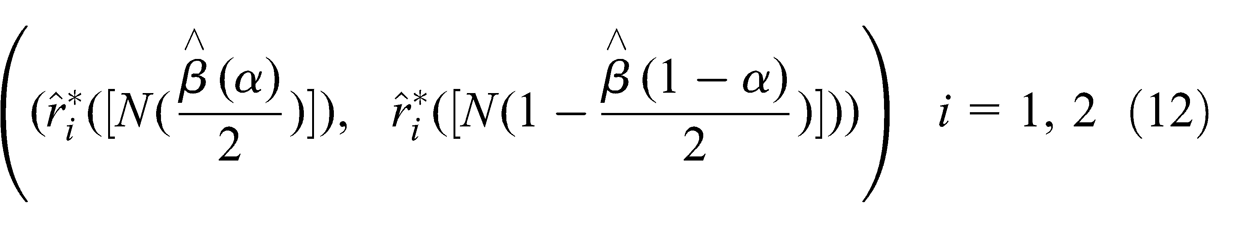
Now call ${\hat{r}}_{i 1}^{*}, {\hat{r}}_{i 2}^{*}, \dots, {\hat{r}}_{iN}^{*}, i = 1, 2$ the bootstrap distribution of ${\hat{r}}_{i}, i = 1, 2$ . Let ${\hat{r}}_{i}^{*} (1), {\hat{r}}_{i}^{*} (2), \dots, {\hat{r}}_{i}^{*} (N), i = 1, 2$ be the order statistics of ${\hat{r}}_{i 1}^{*}, {\hat{r}}_{i 2}^{*}, \dots, {\hat{r}}_{iN}^{*}, i = 1, 2$ . Compute $\overset{\land}{β} (α) = P {r_{i} \leq {\hat{r}}_{i}^{*} ([N (\frac{α}{2})])}$ and $\overset{\land}{β} (1 - α) = P {r_{i} \leq {\hat{r}}_{i}^{*} ([N (1 - \frac{α}{2})])}$ . Then utilizing the $100 (α / 2) th$ and $100 (1 - α / 2) th$ percentage points of the bootstrap distribution, $100 (1 - α) %$ percentile bootstrap (PB) calibrated confidence intervals for $r_{i}$ , i = 1,2 are obtained as

(({\hat{r}}_{i}^{*} ([N (\frac{\overset{\land}{β} (α)}{2})]), {\hat{r}}_{i}^{*} ([N (1 - \frac{\overset{\land}{β} (1 - α)}{2})]))) i = 1, 2

(12)

where [x] denotes the greatest integer less than or equal to x.

10. Bias-corrected and accelerated bootstrap calibrated confidence intervals

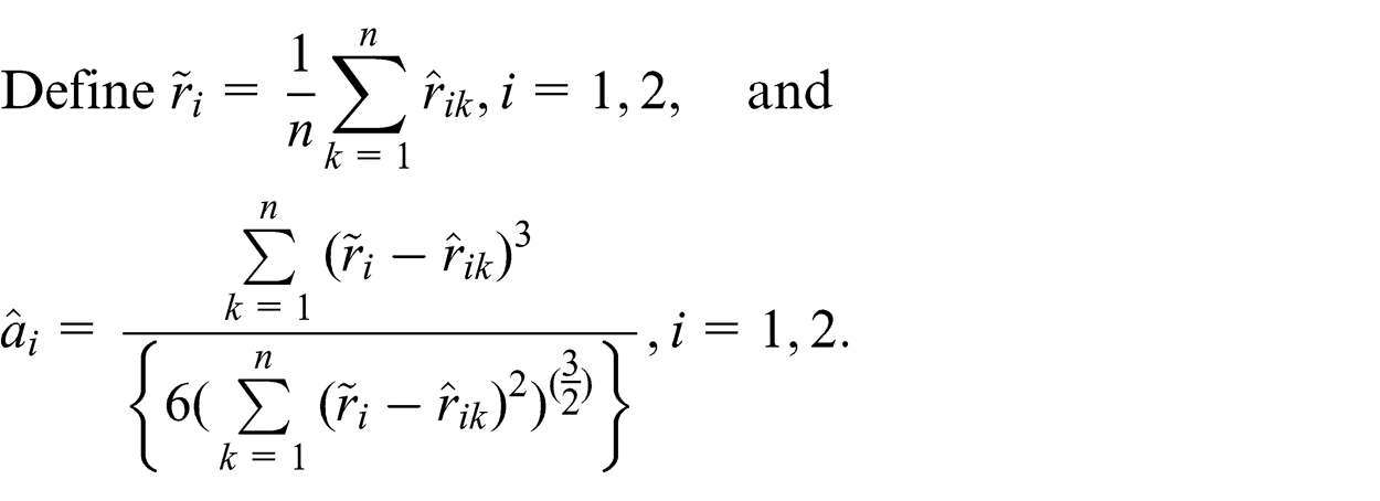
The bootstrap distribution ${\hat{r}}_{i 1}^{*}, {\hat{r}}_{i 2}^{*}, \dots, {\hat{r}}_{iN}^{*}, i = 1, 2$ may be biased. The PB calibrated confidence interval for mean response time is designed to correct this potential bias. Set $p_{i} = \frac{1}{N} \sum_{j = 1}^{N} I ({\hat{r}}_{ij}^{*} < {\hat{r}}_{i}), i = 1, 2$ , where $I (.)$ is the indicator function. Define ${\hat{z}}_{i} = ϕ^{- 1} (p_{i}), i = 1, 2$ , where $ϕ^{- 1}$ denotes the inverse function of the standard normal distribution $ϕ$ . Except for correcting the potential bias of the bootstrap distribution, we can accelerate the convergence of bootstrap distribution. Let $({\tilde{X}}_{i} (k), {\tilde{Y}}_{i} (k), i = 1, 2, k = 1, 2, \dots n)$ denote the original samples with the kth observation $(X_{ik}, Y_{ik}, i = 1, 2)$ deleted; also let ${\hat{r}}_{ik}, i = 1, 2$ be the estimator of $r_{i}$ , i = 1,2 calculated by using $({\tilde{X}}_{i} (k), {\tilde{Y}}_{i} (k), i = 1, 2)$ .

Define {\tilde{r}}_{i} = \frac{1}{n} \sum_{k = 1}^{n} {\hat{r}}_{ik}, i = 1, 2 and {\hat{a}}_{i} = \frac{\sum_{k = 1}^{n} {({\tilde{r}}_{i} - {\hat{r}}_{ik})}^{3}}{{6 (\sum_{k = 1}^{n} {({\tilde{r}}_{i} - {\hat{r}}_{ik})}^{2})^{(\frac{3}{2})}}}, i = 1, 2

${\hat{z}}_{i}$ and ${\hat{a}}_{i}, i = 1, 2$ are named bias-correction and acceleration, respectively. Also compute $\overset{\land}{β} (α) = P {r_{i} \leq {\hat{r}}_{i}^{*} ([N α_{i 1}])}$ and $\overset{\land}{β} (1 - α) = P {r_{i} \leq {\hat{r}}_{i}^{*} ([N α_{i 2}])}$ , where $α_{i 1} = ϕ {{\hat{z}}_{i} + \frac{({\hat{z}}_{i} - z_{\frac{α}{2}})}{1 - {\hat{a}}_{i} ({\hat{z}}_{i} - z_{\frac{α}{2}})}}$ $α_{i 2} = ϕ {{\hat{z}}_{i} + \frac{({\hat{z}}_{i} + z_{\frac{α}{2}})}{1 - {\hat{a}}_{i} ({\hat{z}}_{i} + z_{\frac{α}{2}})}}, i = 1, 2$ .

Thus, $100 (1 - α) %$ bias-corrected and accelerated bootstrap (BCaB) calibrated confidence intervals for $r_{i}$ , i = 1,2 are

({\hat{r}}_{i}^{*} ([N α'_{i 1}]), {\hat{r}}_{i}^{*} ([N α'_{i 2}])), i = 1, 2

(13)

where $α'_{i 1} = φ {{\hat{z}}_{i}' + \frac{({\hat{z}}_{i}' - z_{\frac{\overset{\land}{β} (α)}{2}})}{1 - {\hat{a}}_{i}' ({\hat{z}}_{i}' - z_{\frac{\overset{\land}{β} (α)}{2}})}}$ $α'_{i 2} = φ {{\hat{z}}_{i}' + \frac{({\hat{z}}_{i}' + z_{\frac{(1 - \overset{\land}{β} (1 - α))}{2}})}{1 - {\hat{a}}_{i}' ({\hat{z}}_{i}' + z_{\frac{(1 - \overset{\land}{β} (1 - α))}{2}})}}, i = 1, 2 .$

11. Bias-corrected percentile bootstrap calibrated confidence intervals

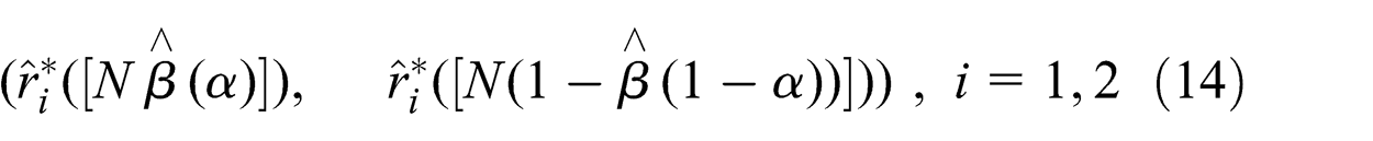
Set $p'_{i} = \frac{1}{N} \sum_{j = 1}^{N} I ({\hat{r}}_{ij}^{*} < {\hat{r}}_{i}), i = 1, 2$ , where I(.) is the indicator function. Define ${\hat{z}}_{i} = ϕ^{- 1} (p'_{i}), i = 1, 2$ , where $ϕ^{- 1}$ denotes the inverse function of the standard normal distribution $ϕ$ . Then $a' = ϕ (2 {\hat{z}}_{i} - z_{α}), i = 1, 2$ and $a ″ = ϕ (2 {\hat{z}}_{i} + z_{α}), i = 1, 2$ . Then compute $\overset{\land}{β} (α) = P {r_{i} \leq {\hat{r}}_{i}^{*} ([Na'])}$ and $\overset{\land}{β} (1 - α) = P {r_{i} \leq {\hat{r}}_{i}^{*} ([Na ″)])}$ . Further 100(1-α)% bias-corrected percentile bootstrap (BCPB) calibrated confidence intervals for mean response time $r_{i}$ , i = 1,2 are

({\hat{r}}_{i}^{*} ([N \overset{\land}{β} (α)]), {\hat{r}}_{i}^{*} ([N (1 - \overset{\land}{β} (1 - α))])), i = 1, 2

(14)

where [x] denotes the greatest integer less than or equal to x.

12. Simulation study

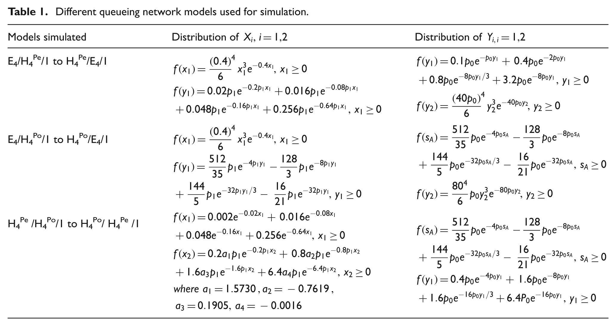
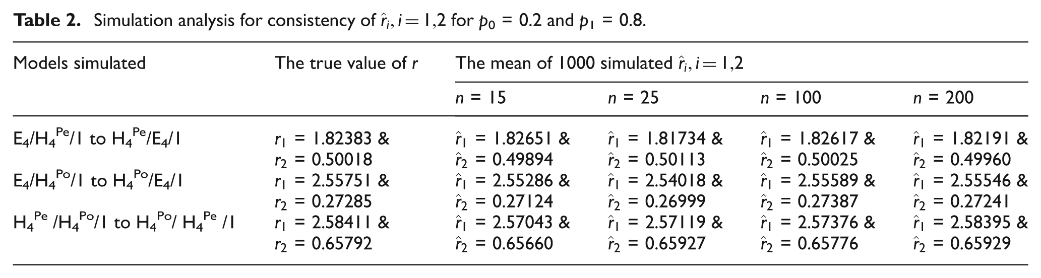
To evaluate performances of calibrated confidence intervals for mean response times of a queueing network with feedback, a numerical simulation study was undertaken. The consistency of $r_{i}$ , i = 1,2 is examined by comparing the true value of $r_{i}$ , i = 1,2 with the average of simulated estimates ${\hat{r}}_{i}$ , i = 1,2, whereas the different calibrated confidence intervals are assessed in terms of their coverage percentages and average length. In order to achieve these goals, we select three different queueing network modes with feedback: E₄/H₄ ^Pe/1 to H₄ ^Pe/E₄/1, E₄/H₄ ^Po/1 to H₄ ^Po/E₄/1 and H₄ ^Pe /H₄ ^Po/1 to H₄ ^Po/ H₄ ^Pe /1, where $E_{4}$ represents a four-stage Erlang distribution, $H_{4}^{Pe}$ a four-stage hyper-exponential distribution and $H_{4}^{P 0}$ a four-stage hypo-exponential distribution.

The distributions of $X_{i}, i = 1, 2$ and $Y_{i}, i = 1, 2$ , as well as the corresponding true mean values of mean response times $r_{i}$ , i = 1,2 for the three different queueing network models, are shown in Tables 1 –3. With regards to E₄/H₄^Pe/1 to H₄^Pe/E₄/1, E₄/H₄^Po/1 toH₄^Po/E₄/1 and H₄^Pe /H₄^Po/1 to H₄^Po/ H₄^Pe /1 queueing network modes with feedback, there is no theoretical formula for the true value of $r_{i}$ , i = 1,2. Using the strong law of large numbers, we have estimated the true value of $r_{i}$ , i = 1,2 by the simulated sample values of ${\hat{r}}_{i}$ , i = 1,2 with sufficiently large sample size. For queueing network models in Table 1, the approximated values of $r_{i}$ , i = 1,2 are obtained from the simulated sample values of ${\hat{r}}_{i}$ , i = 1,2 with sample size n = 10⁷. We find that the approximated mean response time approaches to the true value of $r_{i}$ , i = 1,2 when n≥10⁷.

Table 1.

Different queueing network models used for simulation.

Models simulated	Distribution of $X_{i}, i = 1, 2$	Distribution of $Y_{i, i} = 1, 2$
E₄/H₄ ^Pe/1 to H₄ ^Pe/E₄/1	$\begin{matrix} f (x_{1}) = {\frac{(0.4)}{6}}^{4} x_{1}^{3} e^{- 0.4 x_{1}}, x_{1} \geq 0 \\ f (y_{1}) = 0.02 p_{1} e^{- 0.2 p_{1} x_{1}} + 0.016 p_{1} e^{- 0.08 p_{1} x_{1}} \\ + 0.048 p_{1} e^{- 0.16 p_{1} x_{1}} + 0.256 p_{1} e^{- 0.64 p_{1} x_{1}}, x_{1} \geq 0 \end{matrix}$	$\begin{matrix} f (y_{1}) = 0.1 p_{0} e^{- p_{0} y_{1}} + 0.4 p_{0} e^{- 2 p_{0} y_{1}} \\ + 0.8 p_{0} e^{- 8 p_{0} y_{1} / 3} + 3.2 p_{0} e^{- 8 p_{0} y_{1}}, y_{1} \geq 0 \\ f (y_{2}) = {\frac{(40 p_{0})}{6}}^{4} y_{2}^{3} e^{- 40 p_{0} y_{2}}, y_{2} \geq 0 \end{matrix}$
E₄/H₄ ^Po/1 to H₄ ^Po/E₄/1	$\begin{matrix} f (x_{1}) = {\frac{(0.4)}{6}}^{4} x_{1}^{3} e^{- 0.4 x_{1}}, x_{1} \geq 0 \\ f (y_{1}) = \frac{512}{35} p_{1} e^{- 4 p_{1} y_{1}} - \frac{128}{3} p_{1} e^{- 8 p_{1} y_{1}} \\ + \frac{144}{5} p_{1} e^{- 32 p_{1} y_{1} / 3} - \frac{16}{21} p_{1} e^{- 32 p_{1} y_{1}}, y_{1} \geq 0 \end{matrix}$	$\begin{matrix} f (s_{A}) = \frac{512}{35} p_{0} e^{- 4 p_{0} s_{A}} - \frac{128}{3} p_{0} e^{- 8 p_{0} s_{A}} \\ + \frac{144}{5} p_{0} e^{- 32 p_{0} s_{A} / 3} - \frac{16}{21} p_{0} e^{- 32 p_{0} s_{A}}, s_{A} \geq 0 \\ f (y_{2}) = \frac{80^{4}}{6} p_{0} y_{2}^{3} e^{- 80 p_{0} y_{2}}, y_{2} \geq 0 \end{matrix}$
H₄ ^Pe /H₄ ^Po/1 to H₄ ^Po/ H₄ ^Pe /1	$\begin{matrix} f (x_{1}) = 0.002 e^{- 0.02 x_{1}} + 0.016 e^{- 0.08 x_{1}} \\ + 0.048 e^{- 0.16 x_{1}} + 0.256 e^{- 0.64 x_{1}}, x_{1} \geq 0 \\ f (x_{2}) = 0.2 a_{1} p_{1} e^{- 0.2 p_{1} x_{2}} + 0.8 a_{2} p_{1} e^{- 0.8 p_{1} x_{2}} \\ + 1.6 a_{3} p_{1} e^{- 1.6 p_{1} x_{2}} + 6.4 a_{4} p_{1} e^{- 6.4 p_{1} x_{2}}, x_{2} \geq 0 \\ where a_{1} = 1.5730, a_{2} = - 0.7619, \\ a_{3} = 0.1905, a_{4} = - 0.0016 \end{matrix}$	$\begin{matrix} f (s_{A}) = \frac{512}{35} p_{0} e^{- 4 p_{0} s_{A}} - \frac{128}{3} p_{0} e^{- 8 p_{0} s_{A}} \\ + \frac{144}{5} p_{0} e^{- 32 p_{0} s_{A} / 3} - \frac{16}{21} p_{0} e^{- 32 p_{0} s_{A}}, s_{A} \geq 0 \\ f (y_{1}) = 0.4 p_{0} e^{- 4 p_{0} y_{1}} + 1.6 p_{0} e^{- 8 p_{0} y_{1}} \\ + 1.6 p_{0} e^{- 16 p_{0} y_{1} / 3} + 6.4 P_{0} e^{- 16 p_{0} y_{1}}, y_{1} \geq 0 \end{matrix}$

Table 2.

Simulation analysis for consistency of ${\hat{r}}_{i}, i = 1, 2$ for p ₀ = 0.2 and p ₁ = 0.8.

Models simulated	The true value of r	The mean of 1000 simulated ${\hat{r}}_{i}, i = 1, 2$
Models simulated	The true value of r	n = 15	n = 25	n = 100	n = 200
E₄/H₄ ^Pe/1 to H₄ ^Pe/E₄/1	$r_{1}$ = 1.82383 & $r_{2}$ = 0.50018	${\hat{r}}_{1}$ = 1.82651 & ${\hat{r}}_{2}$ = 0.49894	${\hat{r}}_{1}$ = 1.81734 & ${\hat{r}}_{2}$ = 0.50113	${\hat{r}}_{1}$ = 1.82617 & ${\hat{r}}_{2}$ = 0.50025	${\hat{r}}_{1}$ = 1.82191 & ${\hat{r}}_{2}$ = 0.49960
E₄/H₄ ^Po/1 to H₄ ^Po/E₄/1	$r_{1}$ = 2.55751 & $r_{2}$ = 0.27285	${\hat{r}}_{1}$ = 2.55286 & ${\hat{r}}_{2}$ = 0.27124	${\hat{r}}_{1}$ = 2.54018 & ${\hat{r}}_{2}$ = 0.26999	${\hat{r}}_{1}$ = 2.55589 & ${\hat{r}}_{2}$ = 0.27387	${\hat{r}}_{1}$ = 2.55546 & ${\hat{r}}_{2}$ = 0.27241
H₄ ^Pe /H₄ ^Po/1 to H₄ ^Po/ H₄ ^Pe /1	$r_{1}$ = 2.58411 & $r_{2}$ = 0.65792	${\hat{r}}_{1}$ = 2.57043 & ${\hat{r}}_{2}$ = 0.65660	${\hat{r}}_{1}$ = 2.57119 & ${\hat{r}}_{2}$ = 0.65927	${\hat{r}}_{1}$ = 2.57376 & ${\hat{r}}_{2}$ = 0.65776	${\hat{r}}_{1}$ = 2.58395 & ${\hat{r}}_{2}$ = 0.65929

Table 3.

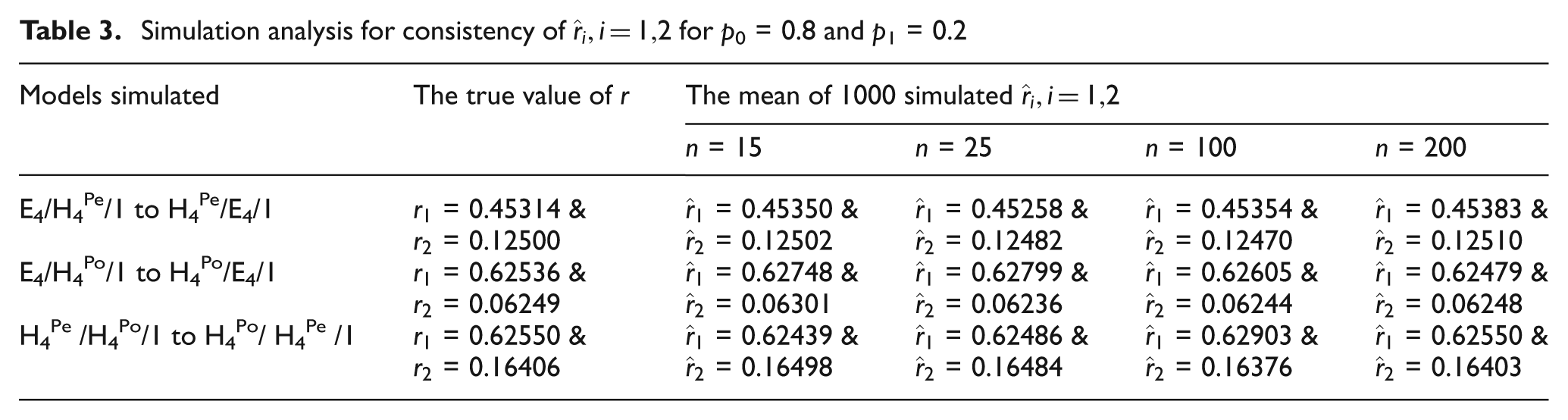
Simulation analysis for consistency of ${\hat{r}}_{i}, i = 1, 2$ for p ₀ = 0.8 and p ₁ = 0.2

Models simulated	The true value of r	The mean of 1000 simulated ${\hat{r}}_{i}, i = 1, 2$
Models simulated	The true value of r	n = 15	n = 25	n = 100	n = 200
E₄/H₄ ^Pe/1 to H₄ ^Pe/E₄/1	$r_{1}$ = 0.45314 & $r_{2}$ = 0.12500	${\hat{r}}_{1}$ = 0.45350 & ${\hat{r}}_{2}$ = 0.12502	${\hat{r}}_{1}$ = 0.45258 & ${\hat{r}}_{2}$ = 0.12482	${\hat{r}}_{1}$ = 0.45354 & ${\hat{r}}_{2}$ = 0.12470	${\hat{r}}_{1}$ = 0.45383 & ${\hat{r}}_{2}$ = 0.12510
E₄/H₄ ^Po/1 to H₄ ^Po/E₄/1	$r_{1}$ = 0.62536 & $r_{2}$ = 0.06249	${\hat{r}}_{1}$ = 0.62748 & ${\hat{r}}_{2}$ = 0.06301	${\hat{r}}_{1}$ = 0.62799 & ${\hat{r}}_{2}$ = 0.06236	${\hat{r}}_{1}$ = 0.62605 & ${\hat{r}}_{2}$ = 0.06244	${\hat{r}}_{1}$ = 0.62479 & ${\hat{r}}_{2}$ = 0.06248
H₄ ^Pe /H₄ ^Po/1 to H₄ ^Po/ H₄ ^Pe /1	$r_{1}$ = 0.62550 & $r_{2}$ = 0.16406	${\hat{r}}_{1}$ = 0.62439 & ${\hat{r}}_{2}$ = 0.16498	${\hat{r}}_{1}$ = 0.62486 & ${\hat{r}}_{2}$ = 0.16484	${\hat{r}}_{1}$ = 0.62903 & ${\hat{r}}_{2}$ = 0.16376	${\hat{r}}_{1}$ = 0.62550 & ${\hat{r}}_{2}$ = 0.16403

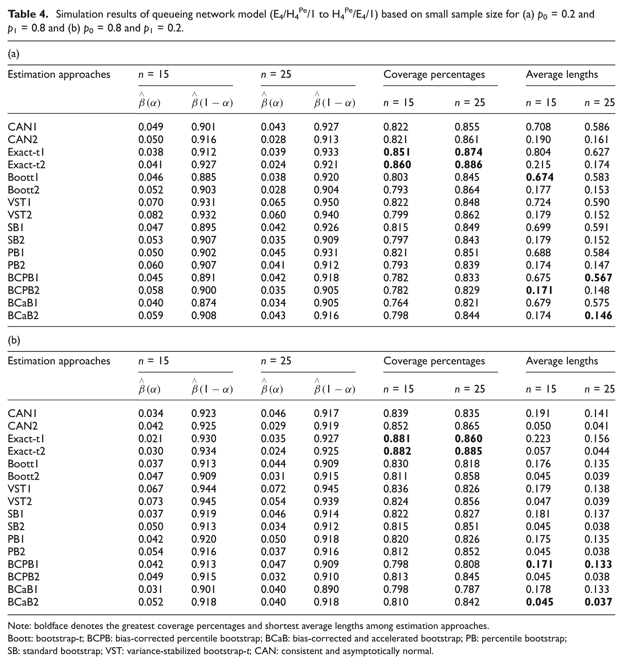
Thus, for each specified queueing network model with feedback in Table 1, a random sample of size n (= 15, 25, 100, 200) is drawn from the original samples. Using recurrence relations (4) and (5), the natural estimates ${\hat{r}}_{i}$ , i = 1,2 are calculated. Further B = 1000 bootstrap re-samples are drawn from the original samples. According to Equations (7)–(14) we obtain CAN/Normal, Exact-t, SB, bootstrap-t (Boott), VST, PB, BCaB and BCPB calibrated confidence intervals for response time $r_{i}$ , i = 1,2 with confidence level 90%. The above simulation process is replicated N = 1000 times and we have computed coverage percentages and average lengths. We utilize Matlab to accomplish all simulations. All simulated results are displayed in Tables 2 –9. The consistency property of the natural estimator ${\hat{r}}_{i}$ , i = 1,2 is demonstrated by Tables 2 and 3, but the performance of the calibrated confidence interval for $r_{i}$ , i = 1,2 can be examined in terms of Tables 4 –9.

Table 4.

Simulation results of queueing network model (E₄/H₄ ^Pe/1 to H₄ ^Pe/E₄/1) based on small sample size for (a) p ₀ = 0.2 and p ₁ = 0.8 and (b) p ₀ = 0.8 and p ₁ = 0.2.

(a)
Estimation approaches	n = 15		n = 25		Coverage percentages		Average lengths
Estimation approaches	$\overset{\land}{β} (α)$	$\overset{\land}{β} (1 - α)$	$\overset{\land}{β} (α)$	$\overset{\land}{β} (1 - α)$	n = 15	n = 25	n = 15	n = 25
CAN1	0.049	0.901	0.043	0.927	0.822	0.855	0.708	0.586
CAN2	0.050	0.916	0.028	0.913	0.821	0.861	0.190	0.161
Exact-t1	0.038	0.912	0.039	0.933	0.851	0.874	0.804	0.627
Exact-t2	0.041	0.927	0.024	0.921	0.860	0.886	0.215	0.174
Boott1	0.046	0.885	0.038	0.920	0.803	0.845	0.674	0.583
Boott2	0.052	0.903	0.028	0.904	0.793	0.864	0.177	0.153
VST1	0.070	0.931	0.065	0.950	0.822	0.848	0.724	0.590
VST2	0.082	0.932	0.060	0.940	0.799	0.862	0.179	0.152
SB1	0.047	0.895	0.042	0.926	0.815	0.849	0.699	0.591
SB2	0.053	0.907	0.035	0.909	0.797	0.843	0.179	0.152
PB1	0.050	0.902	0.045	0.931	0.821	0.851	0.688	0.584
PB2	0.060	0.907	0.041	0.912	0.793	0.839	0.174	0.147
BCPB1	0.045	0.891	0.042	0.918	0.782	0.833	0.675	0.567
BCPB2	0.058	0.900	0.035	0.905	0.782	0.829	0.171	0.148
BCaB1	0.040	0.874	0.034	0.905	0.764	0.821	0.679	0.575
BCaB2	0.059	0.908	0.043	0.916	0.798	0.844	0.174	0.146
(b)
Estimation approaches	n = 15		n = 25		Coverage percentages		Average lengths
Estimation approaches	$\overset{\land}{β} (α)$	$\overset{\land}{β} (1 - α)$	$\overset{\land}{β} (α)$	$\overset{\land}{β} (1 - α)$	n = 15	n = 25	n = 15	n = 25
CAN1	0.034	0.923	0.046	0.917	0.839	0.835	0.191	0.141
CAN2	0.042	0.925	0.029	0.919	0.852	0.865	0.050	0.041
Exact-t1	0.021	0.930	0.035	0.927	0.881	0.860	0.223	0.156
Exact-t2	0.030	0.934	0.024	0.925	0.882	0.885	0.057	0.044
Boott1	0.037	0.913	0.044	0.909	0.830	0.818	0.176	0.135
Boott2	0.047	0.909	0.031	0.915	0.811	0.858	0.045	0.039
VST1	0.067	0.944	0.072	0.945	0.836	0.826	0.179	0.138
VST2	0.073	0.945	0.054	0.939	0.824	0.856	0.047	0.039
SB1	0.037	0.919	0.046	0.914	0.822	0.827	0.181	0.137
SB2	0.050	0.913	0.034	0.912	0.815	0.851	0.045	0.038
PB1	0.042	0.920	0.050	0.918	0.820	0.826	0.175	0.135
PB2	0.054	0.916	0.037	0.916	0.812	0.852	0.045	0.038
BCPB1	0.042	0.913	0.047	0.909	0.798	0.808	0.171	0.133
BCPB2	0.049	0.915	0.032	0.910	0.813	0.845	0.045	0.038
BCaB1	0.031	0.901	0.040	0.890	0.798	0.787	0.178	0.133
BCaB2	0.052	0.918	0.040	0.918	0.810	0.842	0.045	0.037

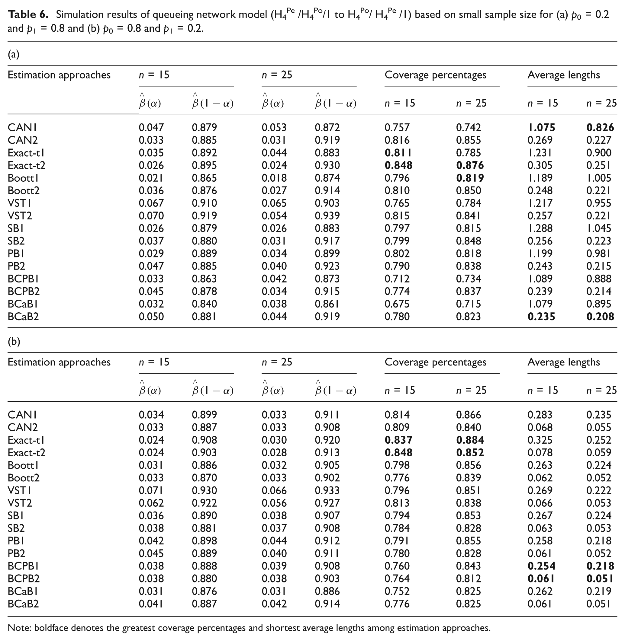
Note: boldface denotes the greatest coverage percentages and shortest average lengths among estimation approaches. Boott: bootstrap-t; BCPB: bias-corrected percentile bootstrap; BCaB: bias-corrected and accelerated bootstrap; PB: percentile bootstrap; SB: standard bootstrap; VST: variance-stabilized bootstrap-t; CAN: consistent and asymptotically normal.

Table 5.

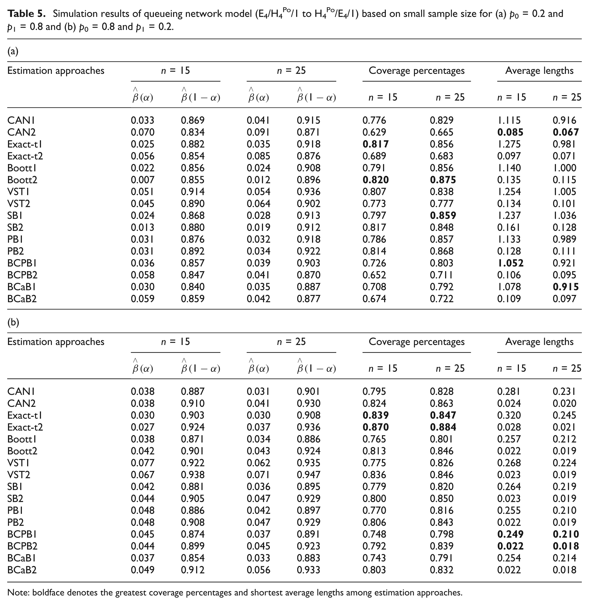
Simulation results of queueing network model (E₄/H₄ ^Po/1 to H₄ ^Po/E₄/1) based on small sample size for (a) p ₀ = 0.2 and p ₁ = 0.8 and (b) p ₀ = 0.8 and p ₁ = 0.2.

(a)
Estimation approaches	n = 15		n = 25		Coverage percentages		Average lengths
Estimation approaches	$\overset{\land}{β} (α)$	$\overset{\land}{β} (1 - α)$	$\overset{\land}{β} (α)$	$\overset{\land}{β} (1 - α)$	n = 15	n = 25	n = 15	n = 25
CAN1	0.033	0.869	0.041	0.915	0.776	0.829	1.115	0.916
CAN2	0.070	0.834	0.091	0.871	0.629	0.665	0.085	0.067
Exact-t1	0.025	0.882	0.035	0.918	0.817	0.856	1.275	0.981
Exact-t2	0.056	0.854	0.085	0.876	0.689	0.683	0.097	0.071
Boott1	0.022	0.856	0.024	0.908	0.791	0.856	1.140	1.000
Boott2	0.007	0.855	0.012	0.896	0.820	0.875	0.135	0.115
VST1	0.051	0.914	0.054	0.936	0.807	0.838	1.254	1.005
VST2	0.045	0.890	0.064	0.902	0.773	0.777	0.134	0.101
SB1	0.024	0.868	0.028	0.913	0.797	0.859	1.237	1.036
SB2	0.013	0.880	0.019	0.912	0.817	0.848	0.161	0.128
PB1	0.031	0.876	0.032	0.918	0.786	0.857	1.133	0.989
PB2	0.031	0.892	0.034	0.922	0.814	0.868	0.128	0.111
BCPB1	0.036	0.857	0.039	0.903	0.726	0.803	1.052	0.921
BCPB2	0.058	0.847	0.041	0.870	0.652	0.711	0.106	0.095
BCaB1	0.030	0.840	0.035	0.887	0.708	0.792	1.078	0.915
BCaB2	0.059	0.859	0.042	0.877	0.674	0.722	0.109	0.097
(b)
Estimation approaches	n = 15		n = 25		Coverage percentages		Average lengths
Estimation approaches	$\overset{\land}{β} (α)$	$\overset{\land}{β} (1 - α)$	$\overset{\land}{β} (α)$	$\overset{\land}{β} (1 - α)$	n = 15	n = 25	n = 15	n = 25
CAN1	0.038	0.887	0.031	0.901	0.795	0.828	0.281	0.231
CAN2	0.038	0.910	0.041	0.930	0.824	0.863	0.024	0.020
Exact-t1	0.030	0.903	0.030	0.908	0.839	0.847	0.320	0.245
Exact-t2	0.027	0.924	0.037	0.936	0.870	0.884	0.028	0.021
Boott1	0.038	0.871	0.034	0.886	0.765	0.801	0.257	0.212
Boott2	0.042	0.901	0.043	0.924	0.813	0.846	0.022	0.019
VST1	0.077	0.922	0.062	0.935	0.775	0.826	0.268	0.224
VST2	0.067	0.938	0.071	0.947	0.836	0.846	0.023	0.019
SB1	0.042	0.881	0.036	0.895	0.779	0.820	0.264	0.219
SB2	0.044	0.905	0.047	0.929	0.800	0.850	0.023	0.019
PB1	0.048	0.886	0.042	0.897	0.770	0.816	0.255	0.210
PB2	0.048	0.908	0.047	0.929	0.806	0.843	0.022	0.019
BCPB1	0.045	0.874	0.037	0.891	0.748	0.798	0.249	0.210
BCPB2	0.044	0.899	0.045	0.923	0.792	0.839	0.022	0.018
BCaB1	0.037	0.854	0.033	0.883	0.743	0.791	0.254	0.214
BCaB2	0.049	0.912	0.056	0.933	0.803	0.832	0.022	0.018

Note: boldface denotes the greatest coverage percentages and shortest average lengths among estimation approaches.

Table 6.

Simulation results of queueing network model (H₄ ^Pe /H₄ ^Po/1 to H₄ ^Po/ H₄ ^Pe /1) based on small sample size for (a) p ₀ = 0.2 and p ₁ = 0.8 and (b) p ₀ = 0.8 and p ₁ = 0.2.

(a)
Estimation approaches	n = 15		n = 25		Coverage percentages		Average lengths
Estimation approaches	$\overset{\land}{β} (α)$	$\overset{\land}{β} (1 - α)$	$\overset{\land}{β} (α)$	$\overset{\land}{β} (1 - α)$	n = 15	n = 25	n = 15	n = 25
CAN1	0.047	0.879	0.053	0.872	0.757	0.742	1.075	0.826
CAN2	0.033	0.885	0.031	0.919	0.816	0.855	0.269	0.227
Exact-t1	0.035	0.892	0.044	0.883	0.811	0.785	1.231	0.900
Exact-t2	0.026	0.895	0.024	0.930	0.848	0.876	0.305	0.251
Boott1	0.021	0.865	0.018	0.874	0.796	0.819	1.189	1.005
Boott2	0.036	0.876	0.027	0.914	0.810	0.850	0.248	0.221
VST1	0.067	0.910	0.065	0.903	0.765	0.784	1.217	0.955
VST2	0.070	0.919	0.054	0.939	0.815	0.841	0.257	0.221
SB1	0.026	0.879	0.026	0.883	0.797	0.815	1.288	1.045
SB2	0.037	0.880	0.031	0.917	0.799	0.848	0.256	0.223
PB1	0.029	0.889	0.034	0.899	0.802	0.818	1.199	0.981
PB2	0.047	0.885	0.040	0.923	0.790	0.838	0.243	0.215
BCPB1	0.033	0.863	0.042	0.873	0.712	0.734	1.089	0.888
BCPB2	0.045	0.878	0.034	0.915	0.774	0.837	0.239	0.214
BCaB1	0.032	0.840	0.038	0.861	0.675	0.715	1.079	0.895
BCaB2	0.050	0.881	0.044	0.919	0.780	0.823	0.235	0.208
(b)
Estimation approaches	n = 15		n = 25		Coverage percentages		Average lengths
Estimation approaches	$\overset{\land}{β} (α)$	$\overset{\land}{β} (1 - α)$	$\overset{\land}{β} (α)$	$\overset{\land}{β} (1 - α)$	n = 15	n = 25	n = 15	n = 25
CAN1	0.034	0.899	0.033	0.911	0.814	0.866	0.283	0.235
CAN2	0.033	0.887	0.033	0.908	0.809	0.840	0.068	0.055
Exact-t1	0.024	0.908	0.030	0.920	0.837	0.884	0.325	0.252
Exact-t2	0.024	0.903	0.028	0.913	0.848	0.852	0.078	0.059
Boott1	0.031	0.886	0.032	0.905	0.798	0.856	0.263	0.224
Boott2	0.033	0.870	0.033	0.902	0.776	0.839	0.062	0.052
VST1	0.071	0.930	0.066	0.933	0.796	0.851	0.269	0.222
VST2	0.062	0.922	0.056	0.927	0.813	0.838	0.066	0.053
SB1	0.036	0.890	0.038	0.907	0.794	0.853	0.267	0.224
SB2	0.038	0.881	0.037	0.908	0.784	0.828	0.063	0.053
PB1	0.042	0.898	0.044	0.912	0.791	0.855	0.258	0.218
PB2	0.045	0.889	0.040	0.911	0.780	0.828	0.061	0.052
BCPB1	0.038	0.888	0.039	0.908	0.760	0.843	0.254	0.218
BCPB2	0.038	0.880	0.038	0.903	0.764	0.812	0.061	0.051
BCaB1	0.031	0.876	0.031	0.886	0.752	0.825	0.262	0.219
BCaB2	0.041	0.887	0.042	0.914	0.776	0.825	0.061	0.051

Note: boldface denotes the greatest coverage percentages and shortest average lengths among estimation approaches.

Table 7.

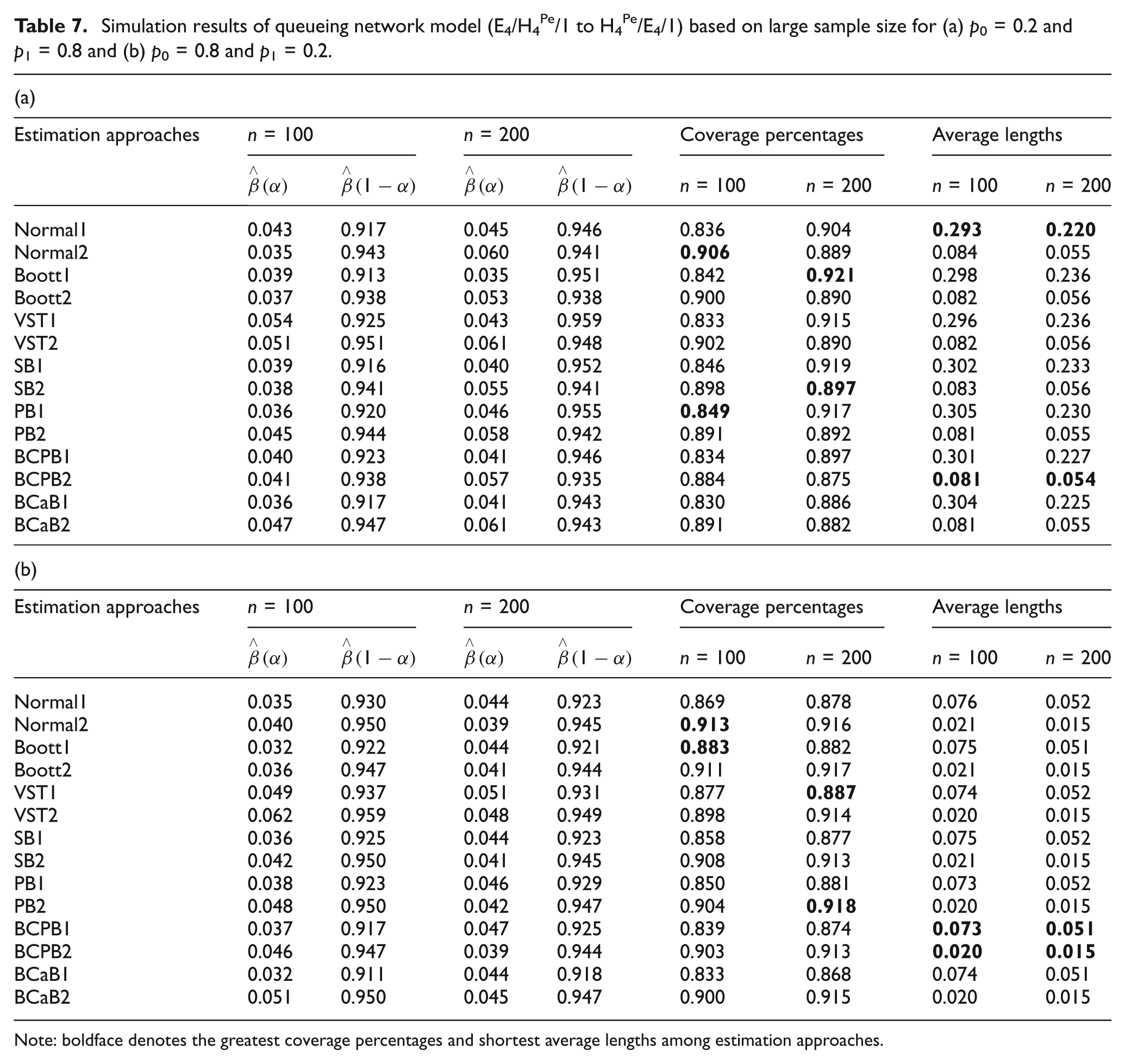
Simulation results of queueing network model (E₄/H₄ ^Pe/1 to H₄ ^Pe/E₄/1) based on large sample size for (a) p ₀ = 0.2 and p ₁ = 0.8 and (b) p ₀ = 0.8 and p ₁ = 0.2.

(a)
Estimation approaches	n = 100		n = 200		Coverage percentages		Average lengths
Estimation approaches	$\overset{\land}{β} (α)$	$\overset{\land}{β} (1 - α)$	$\overset{\land}{β} (α)$	$\overset{\land}{β} (1 - α)$	n = 100	n = 200	n = 100	n = 200
Normal1	0.043	0.917	0.045	0.946	0.836	0.904	0.293	0.220
Normal2	0.035	0.943	0.060	0.941	0.906	0.889	0.084	0.055
Boott1	0.039	0.913	0.035	0.951	0.842	0.921	0.298	0.236
Boott2	0.037	0.938	0.053	0.938	0.900	0.890	0.082	0.056
VST1	0.054	0.925	0.043	0.959	0.833	0.915	0.296	0.236
VST2	0.051	0.951	0.061	0.948	0.902	0.890	0.082	0.056
SB1	0.039	0.916	0.040	0.952	0.846	0.919	0.302	0.233
SB2	0.038	0.941	0.055	0.941	0.898	0.897	0.083	0.056
PB1	0.036	0.920	0.046	0.955	0.849	0.917	0.305	0.230
PB2	0.045	0.944	0.058	0.942	0.891	0.892	0.081	0.055
BCPB1	0.040	0.923	0.041	0.946	0.834	0.897	0.301	0.227
BCPB2	0.041	0.938	0.057	0.935	0.884	0.875	0.081	0.054
BCaB1	0.036	0.917	0.041	0.943	0.830	0.886	0.304	0.225
BCaB2	0.047	0.947	0.061	0.943	0.891	0.882	0.081	0.055
(b)
Estimation approaches	n = 100		n = 200		Coverage percentages		Average lengths
	$\overset{\land}{β} (α)$	$\overset{\land}{β} (1 - α)$	$\overset{\land}{β} (α)$	$\overset{\land}{β} (1 - α)$	n = 100	n = 200	n = 100	n = 200
Normal1	0.035	0.930	0.044	0.923	0.869	0.878	0.076	0.052
Normal2	0.040	0.950	0.039	0.945	0.913	0.916	0.021	0.015
Boott1	0.032	0.922	0.044	0.921	0.883	0.882	0.075	0.051
Boott2	0.036	0.947	0.041	0.944	0.911	0.917	0.021	0.015
VST1	0.049	0.937	0.051	0.931	0.877	0.887	0.074	0.052
VST2	0.062	0.959	0.048	0.949	0.898	0.914	0.020	0.015
SB1	0.036	0.925	0.044	0.923	0.858	0.877	0.075	0.052
SB2	0.042	0.950	0.041	0.945	0.908	0.913	0.021	0.015
PB1	0.038	0.923	0.046	0.929	0.850	0.881	0.073	0.052
PB2	0.048	0.950	0.042	0.947	0.904	0.918	0.020	0.015
BCPB1	0.037	0.917	0.047	0.925	0.839	0.874	0.073	0.051
BCPB2	0.046	0.947	0.039	0.944	0.903	0.913	0.020	0.015
BCaB1	0.032	0.911	0.044	0.918	0.833	0.868	0.074	0.051
BCaB2	0.051	0.950	0.045	0.947	0.900	0.915	0.020	0.015

Note: boldface denotes the greatest coverage percentages and shortest average lengths among estimation approaches.

Table 8.

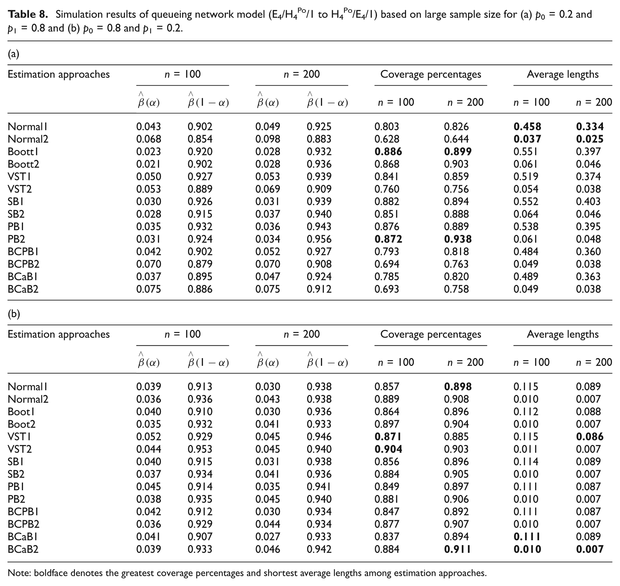
Simulation results of queueing network model (E₄/H₄ ^Po/1 to H₄ ^Po/E₄/1) based on large sample size for (a) p ₀ = 0.2 and p ₁ = 0.8 and (b) p ₀ = 0.8 and p ₁ = 0.2.

(a)
Estimation approaches	n = 100		n = 200		Coverage percentages		Average lengths
Estimation approaches	$\overset{\land}{β} (α)$	$\overset{\land}{β} (1 - α)$	$\overset{\land}{β} (α)$	$\overset{\land}{β} (1 - α)$	n = 100	n = 200	n = 100	n = 200
Normal1	0.043	0.902	0.049	0.925	0.803	0.826	0.458	0.334
Normal2	0.068	0.854	0.098	0.883	0.628	0.644	0.037	0.025
Boott1	0.023	0.920	0.028	0.932	0.886	0.899	0.551	0.397
Boott2	0.021	0.902	0.028	0.936	0.868	0.903	0.061	0.046
VST1	0.050	0.927	0.053	0.939	0.841	0.859	0.519	0.374
VST2	0.053	0.889	0.069	0.909	0.760	0.756	0.054	0.038
SB1	0.030	0.926	0.031	0.939	0.882	0.894	0.552	0.403
SB2	0.028	0.915	0.037	0.940	0.851	0.888	0.064	0.046
PB1	0.035	0.932	0.036	0.943	0.876	0.889	0.538	0.395
PB2	0.031	0.924	0.034	0.956	0.872	0.938	0.061	0.048
BCPB1	0.042	0.902	0.052	0.927	0.793	0.818	0.484	0.360
BCPB2	0.070	0.879	0.070	0.908	0.694	0.763	0.049	0.038
BCaB1	0.037	0.895	0.047	0.924	0.785	0.820	0.489	0.363
BCaB2	0.075	0.886	0.075	0.912	0.693	0.758	0.049	0.038
(b)
Estimation approaches	n = 100		n = 200		Coverage percentages		Average lengths
Estimation approaches	$\overset{\land}{β} (α)$	$\overset{\land}{β} (1 - α)$	$\overset{\land}{β} (α)$	$\overset{\land}{β} (1 - α)$	n = 100	n = 200	n = 100	n = 200
Normal1	0.039	0.913	0.030	0.938	0.857	0.898	0.115	0.089
Normal2	0.036	0.936	0.043	0.938	0.889	0.908	0.010	0.007
Boot1	0.040	0.910	0.030	0.936	0.864	0.896	0.112	0.088
Boot2	0.035	0.932	0.041	0.933	0.897	0.904	0.010	0.007
VST1	0.052	0.929	0.045	0.946	0.871	0.885	0.115	0.086
VST2	0.044	0.953	0.045	0.940	0.904	0.903	0.011	0.007
SB1	0.040	0.915	0.031	0.938	0.856	0.896	0.114	0.089
SB2	0.037	0.934	0.041	0.936	0.884	0.905	0.010	0.007
PB1	0.045	0.914	0.035	0.941	0.849	0.897	0.111	0.087
PB2	0.038	0.935	0.045	0.940	0.881	0.906	0.010	0.007
BCPB1	0.042	0.912	0.030	0.934	0.847	0.892	0.111	0.087
BCPB2	0.036	0.929	0.044	0.934	0.877	0.907	0.010	0.007
BCaB1	0.041	0.907	0.027	0.933	0.837	0.894	0.111	0.089
BCaB2	0.039	0.933	0.046	0.942	0.884	0.911	0.010	0.007

Note: boldface denotes the greatest coverage percentages and shortest average lengths among estimation approaches.

Table 9.

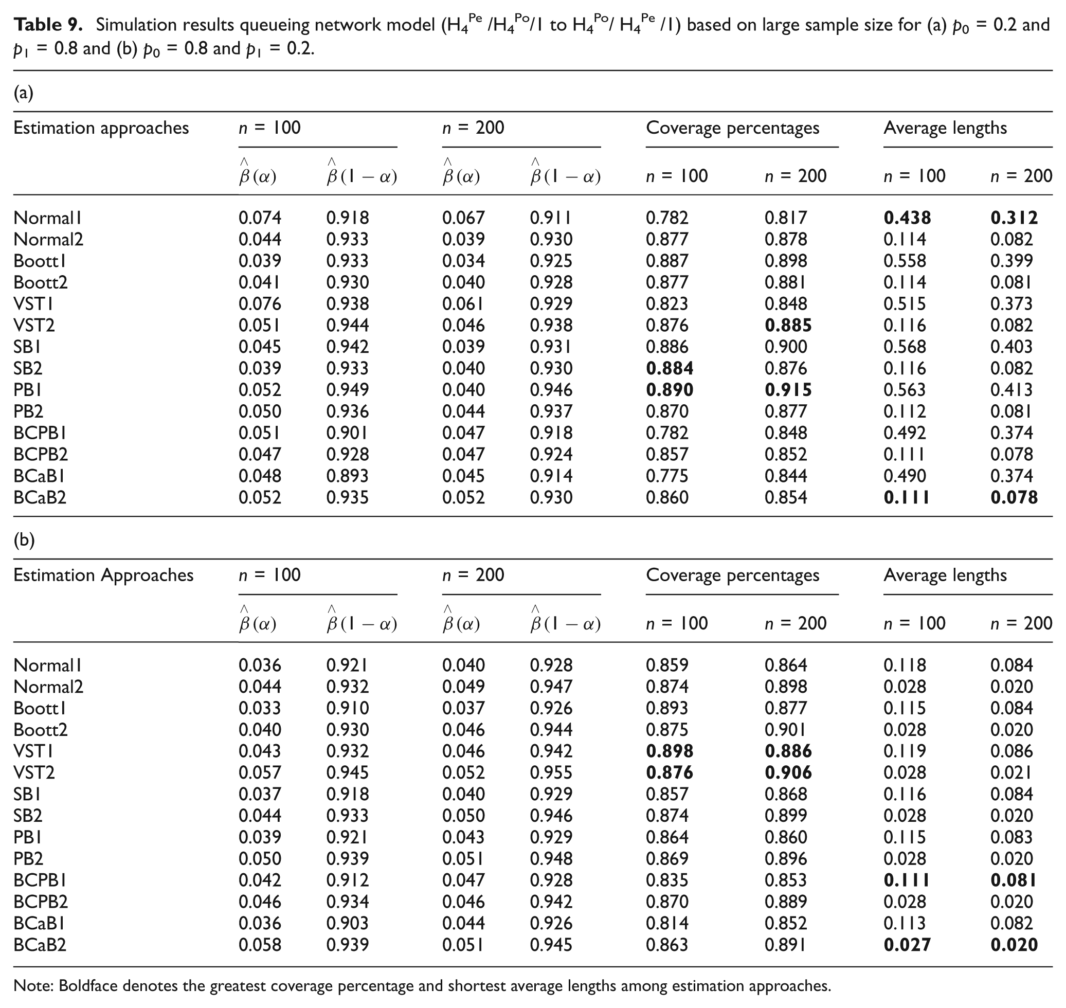
Simulation results queueing network model (H₄ ^Pe /H₄ ^Po/1 to H₄ ^Po/ H₄ ^Pe /1) based on large sample size for (a) p ₀ = 0.2 and p ₁ = 0.8 and (b) p ₀ = 0.8 and p ₁ = 0.2.

(a)
Estimation approaches	n = 100		n = 200		Coverage percentages		Average lengths
Estimation approaches	$\overset{\land}{β} (α)$	$\overset{\land}{β} (1 - α)$	$\overset{\land}{β} (α)$	$\overset{\land}{β} (1 - α)$	n = 100	n = 200	n = 100	n = 200
Normal1	0.074	0.918	0.067	0.911	0.782	0.817	0.438	0.312
Normal2	0.044	0.933	0.039	0.930	0.877	0.878	0.114	0.082
Boott1	0.039	0.933	0.034	0.925	0.887	0.898	0.558	0.399
Boott2	0.041	0.930	0.040	0.928	0.877	0.881	0.114	0.081
VST1	0.076	0.938	0.061	0.929	0.823	0.848	0.515	0.373
VST2	0.051	0.944	0.046	0.938	0.876	0.885	0.116	0.082
SB1	0.045	0.942	0.039	0.931	0.886	0.900	0.568	0.403
SB2	0.039	0.933	0.040	0.930	0.884	0.876	0.116	0.082
PB1	0.052	0.949	0.040	0.946	0.890	0.915	0.563	0.413
PB2	0.050	0.936	0.044	0.937	0.870	0.877	0.112	0.081
BCPB1	0.051	0.901	0.047	0.918	0.782	0.848	0.492	0.374
BCPB2	0.047	0.928	0.047	0.924	0.857	0.852	0.111	0.078
BCaB1	0.048	0.893	0.045	0.914	0.775	0.844	0.490	0.374
BCaB2	0.052	0.935	0.052	0.930	0.860	0.854	0.111	0.078
(b)
Estimation Approaches	n = 100		n = 200		Coverage percentages		Average lengths
Estimation Approaches	$\overset{\land}{β} (α)$	$\overset{\land}{β} (1 - α)$	$\overset{\land}{β} (α)$	$\overset{\land}{β} (1 - α)$	n = 100	n = 200	n = 100	n = 200
Normal1	0.036	0.921	0.040	0.928	0.859	0.864	0.118	0.084
Normal2	0.044	0.932	0.049	0.947	0.874	0.898	0.028	0.020
Boott1	0.033	0.910	0.037	0.926	0.893	0.877	0.115	0.084
Boott2	0.040	0.930	0.046	0.944	0.875	0.901	0.028	0.020
VST1	0.043	0.932	0.046	0.942	0.898	0.886	0.119	0.086
VST2	0.057	0.945	0.052	0.955	0.876	0.906	0.028	0.021
SB1	0.037	0.918	0.040	0.929	0.857	0.868	0.116	0.084
SB2	0.044	0.933	0.050	0.946	0.874	0.899	0.028	0.020
PB1	0.039	0.921	0.043	0.929	0.864	0.860	0.115	0.083
PB2	0.050	0.939	0.051	0.948	0.869	0.896	0.028	0.020
BCPB1	0.042	0.912	0.047	0.928	0.835	0.853	0.111	0.081
BCPB2	0.046	0.934	0.046	0.942	0.870	0.889	0.028	0.020
BCaB1	0.036	0.903	0.044	0.926	0.814	0.852	0.113	0.082
BCaB2	0.058	0.939	0.051	0.945	0.863	0.891	0.027	0.020

Note: Boldface denotes the greatest coverage percentage and shortest average lengths among estimation approaches.

In Tables 2 and 3, the mean of N simulated ${\hat{r}}_{i}$ , i = 1,2 for various n and three specified queueing network models (described in Table 1) are recorded. Tables 2 and 3 imply that the sample mean of ${\hat{r}}_{i}$ , i = 1,2 converges to the true value of $r_{i}$ , i = 1,2 as the sample size n becomes large enough, under any specified queueing network models, as we expect. According to simulation analysis, we show that ${\hat{r}}_{i}$ , i = 1,2 is a consistent estimator of the response times $r_{i}$ , i = 1,2 for queueing network models. All estimates of $\overset{\land}{β} (α) and \overset{\land}{β} (1 - α)$ along with coverage percentages and average lengths of mean response time $r_{i}$ , i = 1,2 based on simulation analysis for different queueing network models with feedback for different interval estimation approaches are shown in Tables 4 to 6 for sample size n = 15, 25 and Tables 7 –9 for sample size n = 100, 200.

According to the simulation results we observe that average lengths are decreasing but coverage percentages are increasing when sample size n increases. The coverage percentage approaches 90% when n increases.

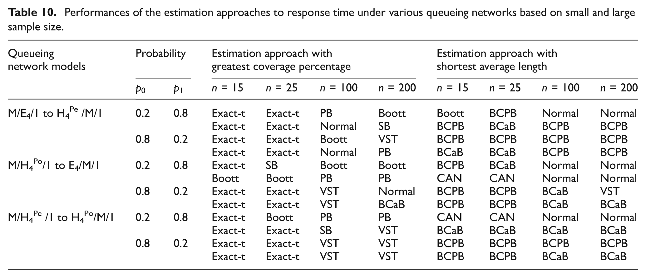
Further, Table 10 shows the comparative study of different estimation approaches. Table 10 is prepared using Tables 4 –9 and it provides estimation approaches with greatest coverage percentage and shortest average length for sample size n (= 15, 25, 100, 200).

Table 10.

Performances of the estimation approaches to response time under various queueing networks based on small and large sample size.

Queueing network models	Probability		Estimation approach with greatest coverage percentage				Estimation approach with shortest average length
Queueing network models	$p_{0}$	$p_{1}$	n = 15	n = 25	n = 100	n = 200	n = 15	n = 25	n = 100	n = 200
M/E₄/1 to H₄ ^Pe /M/1	0.2	0.8	Exact-t	Exact-t	PB	Boott	Boott	BCPB	Normal	Normal
	0.2	0.8	Exact-t	Exact-t	Normal	SB	BCPB	BCaB	BCPB	BCPB
	0.8	0.2	Exact-t	Exact-t	Boott	VST	BCPB	BCPB	BCPB	BCPB
	0.8	0.2	Exact-t	Exact-t	Normal	PB	BCaB	BCaB	BCPB	BCPB
M/H₄ ^Po/1 to E₄/M/1	0.2	0.8	Exact-t	SB	Boott	Boott	BCPB	BCaB	Normal	Normal
	0.2	0.8	Boott	Boott	PB	PB	CAN	CAN	Normal	Normal
	0.8	0.2	Exact-t	Exact-t	VST	Normal	BCPB	BCPB	BCaB	VST
	0.8	0.2	Exact-t	Exact-t	VST	BCaB	BCPB	BCPB	BCaB	BCaB
M/H₄ ^Pe /1 to H₄ ^Po/M/1	0.2	0.8	Exact-t	Boott	PB	PB	CAN	CAN	Normal	Normal
	0.2	0.8	Exact-t	Exact-t	SB	VST	BCaB	BCaB	BCaB	BCaB
	0.8	0.2	Exact-t	Exact-t	VST	VST	BCPB	BCPB	BCPB	BCPB
	0.8	0.2	Exact-t	Exact-t	VST	VST	BCPB	BCPB	BCaB	BCaB

13. Conclusions

This paper provides the comparative study of different calibrated confidence intervals of mean response times $r_{1}$ and $r_{2}$ for a two-stage open queueing network with feedback. Using a recurrence relation approach, we obtain a sequence of response time. The mean of these response times is used as an estimate of the mean response time $r_{i}$ , i = 1,2. This estimator, ${\hat{r}}_{i}$ , i = 1,2, is verified to be consistent by simulation analysis. Different estimation approaches CAN/Normal, Exact-t, SB, Boott, VST, PB, BCaB and BCPB are applied to produce calibrated confidence intervals for mean response times $r_{1}$ and $r_{2}$ . Coverage percentages and average lengths are adopted to understand, compare and assess performance of the resulted calibrated confidence intervals. Table 10 shows performances of the estimation approaches. These approaches are easily applied to practical queueing networks, such as all types of an open, closed and mixed queueing networks, as well as cyclic and retrial queueing models.

Footnotes

Funding

This research received no specific grant from any funding agency in the public, commercial or not-for-profit sectors.

Author biographies

Vinayak K Gedam received his MSc degree in statistics from Rastrasant Tukdoji Maharaj, Nagpur University, Nagpur (India) and his PhD degree in statistics in 2000 from Rastrasant Tukdoji Maharaj, Nagpur University, Nagpur. He joined Sant Gadge Baba Amaravati University, Amaravati (India), as an assistant professor in statistics. Currently he is an associate professor with the Department of Statistics and Centre for Advanced Studies in Statistics, Savitribai Phule Pune University, Pune (India). His research interests include statistical inference (parametric and nonparametric), queueing theory and queueing network models and stochastic transportation problems.

Suresh B Pathare received his MSc degree in statistics (1998) and his MPhil degree in statistics (2004) from Department of Statistics and Centre for Advanced Studies in Statistics, University of Pune (India). Currently he is an assistant professor in statistics at the Indira College of Commerce and Science, Pune. Also he is pursuing his PhD degree from the Department of Statistics and Centre for Advanced Studies in Statistics, Savitribai Phule Pune University, Pune (India). His research interests include statistical inference (parametric and nonparametric), queueing theory and queueing network models.

References

Disney

. Random flow in queueing networks: a review and a critique. Trans AIEE 1975; 7: 268–288.

Jackson

. Networks of waiting lines. Oper Res 1957; 5: 518–521.

Thiruvaiyaru

Basava

Bhat

. Estimation for a class of simple queueing network. Queueing Syst 1991; 9: 301–312.

Kleinrock

. Queueing systems, vol. II, computer applications. New York: John Wiley & Sons, 1976.

Efron

. Bootstrap methods: another look at the jackknife. Ann Stat 1979; 7: 1–26.

Efron

. The jackknife, the bootstrap, and other resampling plans. CBMS-NSF regional conference series in applied mathematics, monograph 38. Philadelphia, PA: SIAM; 1982.

Efron

. Better bootstrap confidence intervals. J Am Stat Assoc 1987; 82: 171–200.

Gedam

Pathare

. Calibrated confidence intervals for intensities of a two stage open queueing network. J Stat Appl Probab 2014; 3: 33–44.

Gedam

Pathare

. Calibrated confidence intervals for intensities of a two stage open queueing network with feedback. J Stat Math 2013; 4: 151–161.

10.

Gedam

Pathare

. Comparison of different confidence intervals of intensities for an open queueing network with feedback. Am J Oper Res 2013; 3: 307–327.

11.

Pathare

Gedam

. Some estimation approaches of intensities for a two stage open queueing network. Stat Optim Inform Comput 2014; 2: 33–46.

12.

Chu

. Confidence intervals of mean response time for an M/G/1 queueing system: bootstrap simulation. Appl Math Comput 2006; 180: 255–263.

13.

Chu

. Interval estimation of mean response time for a G/M/1 queueing system: empirical Laplace function approach. Math Meth Appl Sci 2006; 30: 707–715.

14.

Chu

. Mean response time for a G/G/1 queueing system: simulated computation. Appl Math Comput 2007; 196: 772–779.

15.

Rousses

. A course in mathematical statistics. 2nd ed. New York: Academic Press, 1997.

16.

Hogg

Craig

. Introduction to mathematical statistics. Englewood Cliffs, NJ: Prentice-Hall; 1995.

17.

Efron

Tibshirani

. An introduction to the bootstrap. New York: Chapman and Hall, 1993.

18.

Loh

. Calibrating confidence coefficient. J Am Stat Assoc 1987; 82: 155–162.

19.

Beran

. Prepivoting to reduce level error of confidence sets. Biometrika 1987; 74: 457–468.

20.

Hall

. On the bootstrap and confidence intervals. Ann Stat. 1986; 14: 1431–1452.

21.

Hall

Martin

. On bootstrap resampling and iteration. Biometrika 1988; 75: 661–671.

22.

Loh

. Bootstrap calibration for confidence interval construction and selection. Stat sinica 1991; 1: 477–491.