
Abstract
We introduce an integrated framework for modeling and simulation of ecosystems based on cellular models. The framework integrates cellular modeling, web-based simulation, and geographic information systems (GISs) for data collection and visualization. In this framework, data extraction from GISs is automated; we use the Cell-DEVS formalism for modeling the ecosystem and the CD++ cellular modeling tool within the RISE (RESTful Interoperability Simulation Environment) middleware for web-based simulation. The simulation results are easily integrated with Google Earth data for visualization. We discuss the design, implementation, and benefits of the integrated approach for modeling and simulation in spatial analysis of ecosystem services. We show different case studies in the area of ecological systems, demonstrating how to apply the framework, its usability, and flexibility. We focus on the use of models available in remote servers, their integration with GIS data for inputs, and georeferenced visualization of the results. We show how the modeling methods based on DEVS and their modular interfaces make it easy to build such an architecture and we discuss its application to the field of environmental systems.
1. Introduction
Ecosystems are the life-support systems of the planet, and they are the main source of human life and all other forms of life, providing food, water, clean air, timber, fuel, regulation of infected disease, climate regulation, aesthetic enjoyment, etc. Tansley first defined the term “ecosystem” in 1935 as a system composed of both living organisms and their environments, the chemical–physical components. 1
Unfortunately, ecosystems are in decline around the globe. The Millennium Ecosystem Assessment Report 2005 produced by the United Nations Environment Program states that 60% of the ecosystem services that support life on Earth are being degraded. 2 The effects of agricultural activity and the production of commercial forests cannot be considered separately from environmental and ecological issues. In this light, new technological approaches, methods, and models are needed to address the key factors regarding ecosystem change so as to limit, prevent, or manage ecosystem disruption.
Modeling and simulation is a good way to assess the real system and to predict the expected future of systems that we cannot otherwise test, such as ecosystems, which show a high degree of heterogeneity in space and time. The outcome of the modeling and simulation might also be useful in suggesting management methods to improve the productivity or to control the natural activity of the ecosystem. Modeling and simulation methods have increasingly been used to analyze and understand the properties of ecosystems. 3
Though modeling the dynamics of different applications of ecological system is extremely challenging, a variety of efforts have been presented to define tools and methodologies for modeling and simulation, allowing improved analysis of the complex dynamics of these systems. Of the different approaches, the Discrete Event Systems Specification (DEVS) formalism has become an increasingly accepted modeling framework in this area. 4 The DEVS formalism was defined to specify discrete event systems using a modular description and hierarchical organization. This formalism allows the reuse of tested models, leading to reductions in development and computation time. 5 However, it requires the user to have expertise in advanced programming, distributed programming, etc.
All models of ecological and environmental systems are a simplification of the behavior observed in nature because of ecosystems’ high degree of heterogeneity, periodicity, complexity, dynamicity, geographical coverage, and randomness. There are an enormous number of parameters (about 120,000 parameters 3 ) of interest when modeling ecosystems. Therefore, it is important to select the parameters that are essential to describe the behavior of the system in the context of the problem. To deal with these numerous factors, different methods have been proposed. One of the main methods is the use of spatial representation of the models for ecosystem analysis because it provides efficient and realistic views of the system to users. 6 In this approach, a cell space organizes the structure of the model of a physical system by dividing the area of influence into geometrically distributed cells. The Cell-DEVS formalism and the CD++ toolkit 7 provide a powerful modeling and simulation framework that simplifies the building of these kind complex cellular models by permitting a simple and intuitive model specification. The Cell-DEVS formalism is an extension to define cellular models with explicit timing delays. 8 In Cell-DEVS, a complex system, such as an ecosystem, is described as a space composed of cells, as stated earlier. The Cell-DEVS formalism improves execution performance and ensures the simplicity and reusability of cellular models by using a discrete-event approach. Nevertheless, configuring simulation tools like these might be complex.
In recent years, web-based simulation enabled configuration and reuse issues to be solved by supporting distributed simulation through the World Wide Web. Some other benefits of web-based simulation include visualization of the simulation results, scalability, and global cooperation of the community. Therefore, web-based simulation can be useful for improving modeling and simulation of ecosystems effectively. However, many web-based simulation systems are under the control of single team or a closed community, using interfaces that are tied to their implementation.9,10 Instead, the RESTful Interoperability Simulation Environment (RISE) middleware10,11 uses RESTful web services to hide all the functionalities in resources named with uniform resource identifiers (URIs). These URIs are connected to each other via uniform virtual channels in which simulation synchronization is achieved via XML messages using hypertext transfer protocol (HTTP) methods. The DCD++ environment 12 is an extension of the CD++ environment that enables distributed simulation of DEVS and Cell-DEVS models, and it has been integrated under the RISE middleware. Using RISE, DEVS and Cell-DEVS models can be run in a remote server running parallel simulation algorithms, like those presented by Liu and Wainer 13 in parallel architectures, and providing the results to be integrated with other software components remotely using web-based simulation services.
Web-based simulation environments enable the integration of existing web services with modeling and simulation. However, ecological and environmental modeling and simulation are influenced by spatial relationships, and the analysis of such simulation results faces difficulties in the interpretation of data and in conveying the results clearly to the users. 14 For these applications, geographic information systems (GISs) and their associated data visualization technologies can play an important role by solving the aforementioned difficulties. These GIS software applications are used for capturing, storing, retrieving, manipulating, and visualizing spatially or geographically referenced data. Currently, GISs can be used to manage large amounts of geographically related information, and for manipulating data, performing analysis, and visualization. They are usually organized in several layers of data and make the data accessible in several forms, such as maps or raw data. Modeling and simulation tools can benefit from the use of geographical data, especially when simulating environmental and ecological applications and, in particular, the ones that we are interested in modeling here: agriculture, forestry, minerals, climate, pollution, spread of disease, urban planning, etc. Hence, interfacing between GISs and simulation models is an important means to explore the potential of GISs for performing interactive analysis.
For ecosystem simulations, it would be very effective if the inputted data came directly from GIS software. Conversely, it is also useful if the simulation results are displayed using an appropriate geospatial visualization system. Geospatial visualization systems allow the behavior results of the environmental applications under study to be viewed; therefore, we can evaluate the potential environmental impacts more rigorously. For instance, Google Earth is a geospatial visualization system that can be used to visualize and evaluate simulation results. Google Earth provides the capability of integrating satellite images, aerial photography, and digital map data into a three-dimensional interactive virtual template of the world. 15
Based on these considerations, our objective is to define a web-based integrated architecture for modeling, simulation, and visualization of ecosystems using Cell-DEVS to explore and forecast the behavior for supporting the decision making. The basic idea is to provide a framework that combines GIS data collection, modeling, and simulation using DEVS and Cell-DEVS theory, remote execution using web-based simulation, and visualization of the results using a geospatial visualization system (in our examples, we have used Google Earth), allowing the users to choose the best available technologies to analyze the ecosystem behavior for future policy decisions. The GIS data collection process is done automatically by generating initial value files for the Cell-DEVS model from GIS data. The multi-layer definition of GIS raw data can be directly imported into multi-layer Cell-DEVS models, like the models presented in the following sections. To understand the use of the architecture with practical uses, we show different prototype applications using the proposed integrated framework. In this framework, Cell-DEVS is used as an abstract formalism that enables the separation of modeling and simulation; the RISE middleware also decouples simulator implementation from underling hardware, while web-based simulation is the coupling of modeling and simulation with the Web; as a result, the system becomes ideal for online deployment.
The rest of the paper is organized as follows. Section 2 provides information about the related works in web-based distributed simulation in the domain of the DEVS and Cell-DEVS formalisms. Section 3 describes briefly about the Cell-DEVS modeling and simulation environment. In this section, we also present two case studies, so that one can get a clear idea of how to model and simulate using the CD++ tool in the Cell-DEVS environment. The objective of this section is to present a set of ecological models and to show how to model them with the Cell-DEVS methodology. These models then reside in a remote server and can be reused within the context of our simulation environment, which is presented in Section 4. Here, we present the integration of web-based simulation and GIS visualization, showing how to use initial data obtained in GIS systems and how to improve their visualization using remote simulation through web services. Section 5 presents an illustrative example that describes a complete web-based simulation and GIS visualization process using the integrated architecture. Finally, Section 6 provides conclusions.
2. Background
The use of web-based integrated platforms for modeling, simulation, and visualization of ecological and environmental systems has a number of advantages. Integrating GISs, modeling, web-based simulation, and visualization allow the definition of a complex software application with distinct features. The GIS can be used to collect and manage spatial information. Modeling allows the representation of the dynamic relationships among studied entities in order to predict behavior. Web-based simulation eases the implementation of simulation and reuse using web technologies. 16 Finally, visualization allows presentation of the simulation results in an intuitive way for fast decision making, enhancing the communication of results to non-technical users.
In recent years, many simulation models in the area of environmental systems have been developed using cellular automata (CA) formalism.17,18 This formalism provides a good mechanism to represent spatial information. The CA formalism defines a model as an infinite regular n-dimensional lattice of cells. The state of these cells is updated in discrete time-steps according to local rules in a synchronous fashion. The CA are consistent with the concept of unified space–time and can handle boundary and initial conditions, inhomogeneities and isotropies of a dynamic system 19 ; many ecological models have been built with CA because of these properties. For instance, Chen and Mynett 20 developed a two-dimensional CA model (EcoCA) to approximate prey–predator behavior. DINAMICA 21 is a CA model focusing on the development of spatial patterns produced by landscape dynamics. This model is also useful to investigate many other types of environmental dynamic phenomena.
However, CA can be restricted by the simplicity of their formal description. The CA also frequently need to be modified for simulation purposes.7,22 They use a discrete time base for cell updates, which restrains the precision and efficiency of the simulated models. Therefore, although CA can form a useful tool to model systems when space, time, and states are discrete, they cannot adequately describe most physical systems whose nature is asynchronous. All these issues constrain their power, performance, usability, and feasibility to analyze complex systems, such as ecosystems. In our earlier work,7,8 we discussed how, in spite of widespread use and capability, CA models can be computationally inefficient in studying complex systems.
Another well-defined formal modeling and simulation methodology is DEVS. 4 This is a modeling and simulation formalism based on dynamic systems theory. The DEVS models are organized hierarchically, using modular descriptions and supporting discrete-event approximation of continuous systems. Because of these factors, DEVS has been used for modeling ecosystems. Bergez et al. 23 developed an open DEVS platform to model, simulate, and evaluate agro-ecosystems. 24 CRASH (Crop Rotation and Allocator Simulator using Heuristics) is a modeling framework based on DEVS, which integrates a set of tools to plan, simulate, and analyze cropping-plan decision making in an uncertain environment at the farm scale. 25 In environmental applications, cellular propagations are numerous. The large volume of data and complexity of such a type of models required easy design, modification, and efficiency in terms of execution time. Muzy et al. 26 showed that DEVS could be used with discrete-event hierarchical modeling to deal with these issues, which facilitates construction, maintenance, and reusability of the simulation, while reducing the calculation time.
A real system modeled using DEVS can be described as a composition of atomic and coupled components. An atomic model represents a part of the system that describes the autonomous behavior of the discrete event system as a sequence of deterministic transitions between states in response to the triggering of events. A coupled model is composed of several atomic or coupled submodels; these are interconnected through the model’s interface. The DEVS formalism includes well-defined coupling of components, modular construction, and support for repository reuse.
The Cell-DEVS formalism 27 combines both approaches: CA and DEVS. It allows the definition of cellular models with explicit timing delays, allowing the problems discussed to be overcome. A Cell-DEVS model is a lattice of cells, where each cell is a DEVS atomic model and cell space as a coupled model. Each Cell-DEVS atomic model holds a state variable and a computing function that updates the cell state. This is done by using the present cell state and those of a finite set of nearby cells (called the neighborhood). The efficient computation of cell state variations and the I/O port mechanisms of Cell-DEVS allow for the development of all larger models and for the faster execution of models. It also provides straightforward integration of the models with other modeling formalisms.
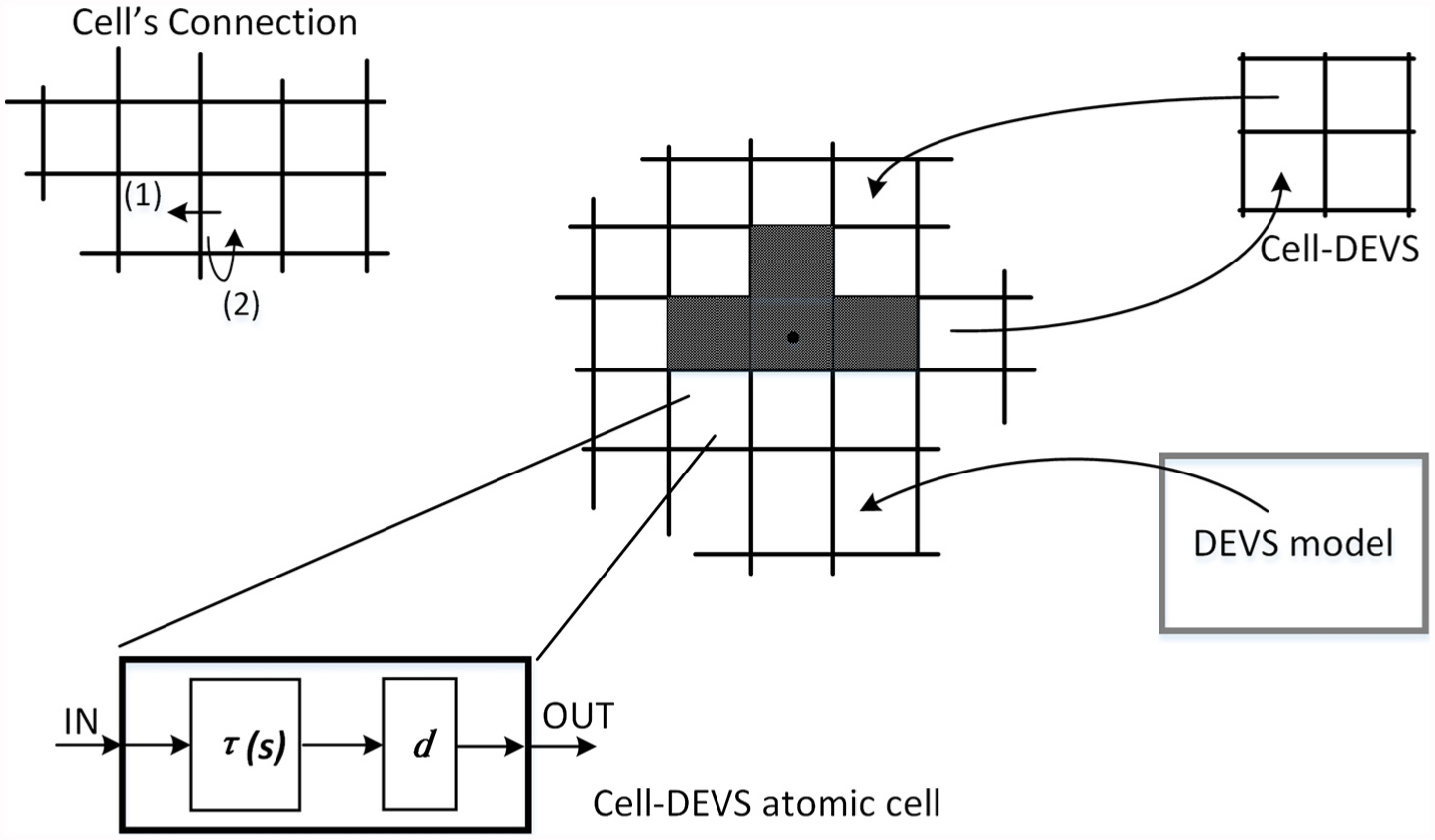
Figure 1 describes the basic concept of a Cell-DEVS model. A Cell-DEVS atomic model is defined formally as 27 :

Where X is a set of external input events, Y is a set of external output events, S is the set of states, delay is the transport or inertial delay, d is the transport delay for the cell, δint and δexit are the internal and external transition functions respectively, τ is the local computing function, λ is the output function, and D is the lifetime function of the state. A Cell-DEVS coupled model is formally defined as:

Where Xlist and Ylist are the input and output coupling lists, respectively, X and Y are the set of external input and output events, respectively, n is the dimension of the cell space, {t1, …, tn} are the number of cells in each of the dimensions, N is the neighborhood set, C is the cell space, B is the border cells set, and Z is the translation function. A Cell-DEVS atomic model uses a set of inputs to compute its future state from the state set using the local computing function τ(S). These results are transmitted after a delay d (with different semantics for the delay function). After the basic behavior of a cell is defined, a coupled model is defined to integrate the atomic models representing the cell space. A Cell-DEVS coupled model is an array of atomic cells, each connected to a set of neighboring cells and potentially to other external DEVS or Cell-DEVS models.
Definition of Cell-DEVS. 5
CD++ is an open-source modeling and simulation tool that provides a development environment for implementing DEVS and Cell-DEVS. 27 DEVS atomic models can be developed and integrated onto a basic class hierarchy programmed in C++. Coupled models can be defined using a built-in specification language based on the formal specifications of Cell-DEVS. The model specification includes the definition of the size and dimension of the cell space, borders, and the shape of the neighborhood. The cell’s local computing function is defined using a set of rules with the form “postcondition assignments delay {precondition}.” 5 When the precondition is satisfied, the state of the cell will change to the designated postcondition, whose values will be transmitted to other components after the delay. If the precondition is false, the next rule in the list is evaluated until a rule is satisfied or there are no more rules. If the model’s state variables need to be modified, the assignments section can be used. CD++ interprets this specification language and executes a simulation of the model.
We used Cell-DEVS to create various environmental models. One of these focuses on forest fires depending on the fuel, the geography of the area, the weather etc. 28 In an earlier study, 5 we presented different models showing how to define simple applications using Cell-DEVS theory and CD++. Koutitas et al. 29 studied two wildfire models, one (InteSys) based on CA and another (CD-AUTH) based on Cell-DEVS. Ecological models are distributed and show heterogeneity in time and space with a large volume of data and operations. Muzy et al. 22 proposed a framework for modeling and simulating ecological propagation processes. Mittal et al. 30 presented a distributed modeling and simulation framework called DEVS/SOA, which supports a development and testing environment. This framework also aims to develop and evaluate distributed simulation under the web environment. In the following sections, we will show detailed case studies developed using Cell-DEVS and will discuss the advantages in modeling ecosystems.
When the complexity and dynamicity of the models increase, we need more resources for the simulation and more complex tools needing special configuration. Sharing models and reusing simulations is usually complicated. At the same time, the Internet provides a common platform for integrated resources. This resulted in the definition of web-based simulation services, i.e., the invocation of computer simulation services over the World Wide Web. Web-based simulations have made use of the simple object access protocol (SOAP), for exchanging information between peers in a decentralized, distributed environment using XML. Interfacing with SOAP web services is done in the form of programming functions that are implementation-specific, and SOAP messages in XML are exchanged at the web service technology layer (and not at the simulation level). Therefore, although SOAP-based distributed simulation protocols support interoperability; this is at a cost of increased complexity. 10 Instead, RESTful web services 11 do not have these problems: Representational State Transfer (REST) is usually implemented using HTTP, URIs, and XML, and integration is easier. Resources are named (addressed) with unique URIs similar to website URLs, and are connected through HTTP channels. REST can separate internal implementation from interface semantics. 11
Based on these ideas, in our earlier work,9,10,11 we designed and implemented RISE middleware. It serves as a container to hold different simulation environments without being specific to any of them. We also showed10,31 that implementation of CA within the RISE-based distributed CD++ can improve interoperability and performance, compared with other similar environments. RISE improved the infrastructure for distributed processing of web-based simulation models, giving us the chance to use the different web services available, including those providing real-time geospatial data. Geographic information systems provide the means for manipulating georeferenced information and performing different operations with maps. In GISs, data are organized in a number of layers, centralizing all the environmental data available and making the data accessible in different formats. Many studies have demonstrated the efforts to integrate the GIS, simulation modeling, and visualization. For instance, Virtual Fire 32 is a real-time platform for forest fire control that integrates GIS, simulation modeling, and visualization for fire management. CyberGIS Software Integration for Sustained Geospatial Innovation 16 focuses on the integration of cyber-infrastructure, the GIS, and simulation modeling for computationally intensive spatial data analysis and collaborative geospatial problem-solving and decision making that can be simultaneously conducted by a large number of users. Sun et al. 15 shows the design and implementation of a web-based visual, interoperable, and scalable platform that is able to manage and visualize vast amounts of distributed, heterogeneous, and model data and images for climate study using GIS and Google Earth. Kulkarni et al. 33 presented an integrated web and GIS-based flood assessment model to provide web-enabled two-dimensional flood simulation, visualization, and analysis of flooding in coastal areas. The Group on Earth Observation Model Web 34 is an environmental model access and interoperability tool focusing on four basic principles: open access, minimal barriers to entry, service-driven development, and scalability.
In this research, we have used an open-source GIS tool, the Geographic Resources Analysis Support System (GRASS). 35 GRASS uses GeoTIFF, an open standard to establish a TIFF-based interchange format for georeferenced raster images. In Wang and Wainer 36 and Zapatero et al., 37 we showed how to map GIS data into CD++. The basic idea is to map the geoinformation from real-world geo-ordinates to cell space ordinates, convert the whole region into cells, and store the cells in the initial value fine for Cell-DEVS simulation.
The integration between modeling, simulation and visualization can significantly increase the strength of representation that results in ease of understanding the simulation results. Examples of this includes the ArcView Non-Point Source Pollution Modeling tool, 38 which was built to facilitate agricultural watershed modeling. Sun et al. 15 presented the design and implementation of a web-based visual, interoperable, and scalable platform for climate research. Google Earth has evolved significantly in recent years and is used for both scientific and generic purpose. It uses the keyhole markup language (KML), an open standard from the Open Geospatial Consortium, which uses XML for geographic visualization that includes annotation of maps and images. Google Earth provides mechanisms to make layers evolve forward and backward in time, which is useful to analyze the progress of a simulation interactively. In our earlier work, 37 we used Google Earth as the geospatial visualization system.
In light of these considerations, we investigated the use of Cell-DEVS for environmental or ecological applications. We defined an architecture combining GIS data collection, modeling with Cell-DEVS, web-based simulation using RISE middleware, and visualization of the results in Google Earth. Our GIS data collection and visualization processes are automated subsystems that generate initial data files for simulation engines and KML files for GIS visualization. Cell-DEVS is an abstract formalism that provides many advantages for modeling environmental applications. Finally, the RISE middleware allows the implementation of web-based simulation. In the next section, we discuss details of the Cell-DEVS modeling and simulation based on environmental applications. Section 4 presents detailed architecture of the integrated platform. In Section 5, we present a complete ecosystem model implemented using this platform.
3. Cell-DEVS modeling and simulation of environmental models
In this section, we give a brief introduction of the complete integrated Cell-DEVS modeling and simulation cycle. We use a software architecture with four components, as shown in Figure 2.
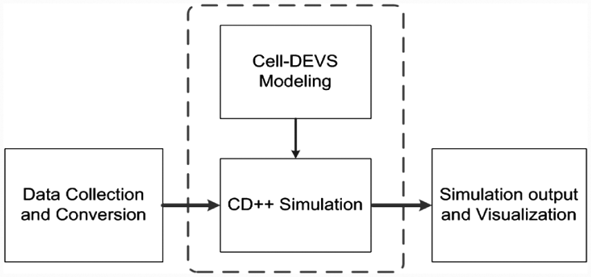
Simplified Cell-DEVS simulation architecture.
The data collection and conversion subsystem gathers initial GIS data and converts and stores them as initialization data for the CD++ model. In ecosystem or environmental applications, this subsystem maps the geoinformation from real-world geo-ordinates to cell space ordinates, converts the whole region into cells, and stores them as initial value files for the CD++ simulator. The visualization subsystem takes the simulation results as input, parses the results, optimizes them, and generates a KML file to visualize the output (for instance, using Google Earth). The models are designed using the Cell-DEVS formalism and simulated in the CD++ environment. We use RISE to execute the CD++ simulations remotely. The GIS software manages spatial information and the interactive visualization enhances a user’s ability to better understand the studied phenomenon, provide interactive environment to verify models, and refine the model for different scenarios. The integration of Cell-DEVS and the GIS will provide many advantages, such as the reusability of models, the simple rule-based nature of entity behavior definition, asynchronous model execution that improves the execution speed, and I/O ports for interfacing different models and data transfer between different spatial components. We will show those advantages by studying different case studies for application of the methodology. Moreover, through the following case studies, we show how the modeler can use our web-based open-source tool for modeling and simulation, as mentioned earlier. In Section 4, we discuss, in detail, the architecture of the integrated framework for web-based simulation and visualization.
3.1. A model for the effect of the mountain pine beetle
The mountain pine beetle is native to western North America, from northern Mexico to northern British Columbia, Canada. It has also significantly expanded its range in the Rocky Mountains, Alberta, and Saskatchewan. This small beetle primarily infects lodgepole pine trees and kills millions of cubic feet of commercial tree species (also sugar pine, western white pine, etc.). It is estimated that the mountain pine beetle killed 283 million cubic meters of pine trees in British Columbia from 1990 to 2005. 39 It also increased the risk of large fires with dead and dying trees. Currently, the industry’s best practices are to clear cut any forest infected with mountain pine beetle to slow or stop infestation in the surrounding area (losing revenue).
We defined an extension of the CA presented by Bone et al. 39 in Cell-DEVS. The model includes various types of forest feature (a river, a lake, an incomplete clear cut, etc.), with the goal of demonstrating how to conduct analysis and modeling for improving forest management practices using Cell-DEVS. We are using a model that has been validated by environmental science researchers; Bone et al. 39 have carried out validation activities. The objective of this section is to show an implementation of such model and the rules defined by the initial research using the Cell-DEVS formalism. The modeling rules are a direct translation of the rules found in the original paper. The objective here is to show researchers interested in environmental sciences how to translate similar models into Cell-DEVS versions, with the objective of being able to make use of our architecture for integration of web-based simulation and visualization.
The original CA model for mountain pine beetle attack involves looking at the tree susceptibility value for each forest unit, which is obtained by multiplying the size (S) of the trees in the unit, the proportion (P) of lodgepole pine trees, the density (D) of trees, and the location factor (L), which represents the proximity to a known infestation. Size S reflects the fact that larger trees are more susceptible to infestation; P and D reflect the fact that mountain pine beetles only infect pine trees and tend to do better in dense forests. The parameter L represents the beetle’s ability to move; places closer to infestations are more likely to become infected. Once these parameters are defined, an allometric function (y = 0.05x−1.3) is used to determine the tree mortality. This function defines the number of mountain pine beetles required in the neighborhood for a tree with a given level of susceptibility to become attacked. It follows the logic that trees with high susceptibility require low levels of mountain pine beetle in the neighborhood to become attacked, and as mountain pine beetle populations increase to higher levels they attack less susceptible trees. Once a cell is infected, there is a 100% certainty that all the lodgepole pines in the area will eventually be infected. Empirical evidence suggests that up to 80% of mountain pine beetles in a given tree will die during the winter (i.e., each generation has 80% mortality).
The model (Figure 3) is defined as follows.
It includes a two-dimensional map that could include rivers, lakes, clear-cuts, etc.
It defines the state of the trees in the forest: alive, infected, and dead.
Each tree is only affected by trees in its neighborhood.
If a tree stand is alive, we compute the number of mountain pine beetles in the stand.
If the total concentration of mountain pine beetles is larger than the allometric function, the stand becomes infected and it dies before the next season.
Mountain pine beetles move through the forest and are computed as the average concentration for the surrounding cells plus the current number of beetles less the number that died during the winter.
Trees cannot recover from a mountain pine beetle infestation.
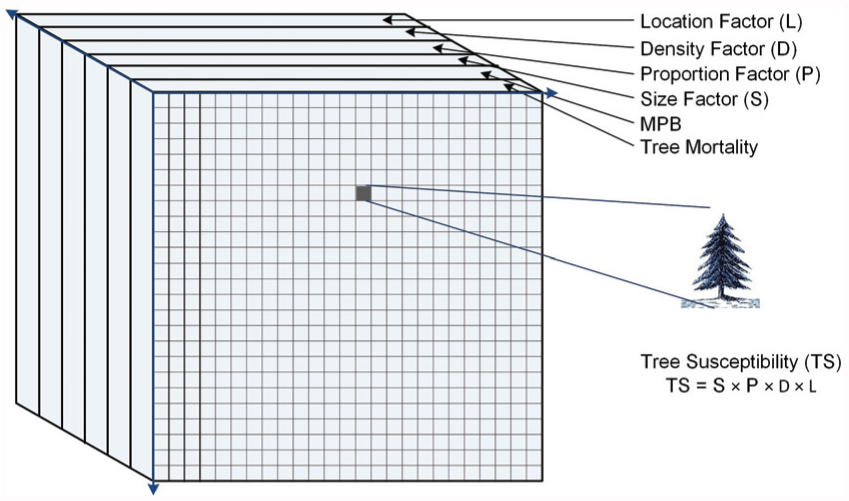
Model organization and model layers or state variables.
The model has been built using a multi-layer approach (six layers) representing different phenomena on each layer.
Mortality. This represents the trees that have been killed by mountain pine beetle.
Mountain pine beetle. This represents the movement of the mountain pine beetles and their relative concentration in any given cell.
Susceptibility factors. These are size, density, proportion, and location factors for a given stand.
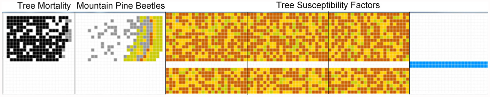
The Cell-DEVS we will show in Figures 4 to 6 include six planes with 25 cells × 25 cells. All the cells in the mortality plane (plane 0) are initially set to zero. Plane 1 is the mountain pine beetle layer; it has one cell initially and contains all zeros except for places where it is desired that no trees grow (these are set to 1). The density, size of the tree, and proportion are generated randomly. The rules for each plane are based on the preceding equation, and are defined as shown in Figure 4.
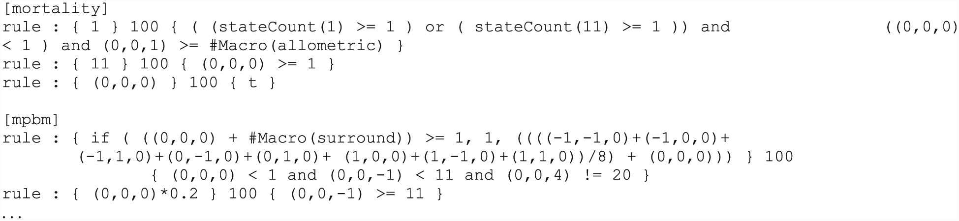
Mountain pine beetle epidemic model specification.
River and forest model.
Model with incomplete clear cut.
Figure 4 shows some sample rules defined in different layers in the model. In the first rule, we use
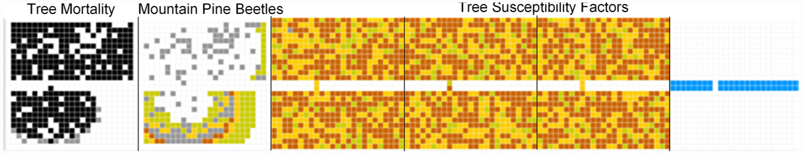
Figures 5 and 6 show the six layers, showing different aspects of the simulation. The first layer represents the tree mortality (showing dead trees); the second square shows the number of mountain pine beetles (as a concentration). The remaining squares show the three susceptibility factors discussed earlier. A color code has been used to identify different aspects: white for trees in good health (not infected), dark gray for infected trees, black for dead trees, blue for river, dark orange for high susceptibility, orange for moderate susceptibility, and lemon for low susceptibility.
Figure 5 shows a model with a source of highest concentration of mountain pine beetles at (1, 1) and a forest bisected by a river (which the mountain pine beetles are unable to cross). The figure shows an intermediate step with the progression of the epidemic impeded by the river.
Figure 6 presents the results when the simulation includes an incomplete clear cut. In this case, it is shown that the beetles are capable of traveling across the unclear cut land, and affect the trees on the other side. This example is of critical importance to the simulation of the effects of clear cutting forests for prevention of mountain pine beetle outbreaks.
3.2. Modeling the impact of the diamondback moth
The diamondback moth is a pest native to Europe that was introduced into North America about 150 years ago. It can now be found almost all over the world, and is one of the world’s most destructive crop pests. Around $1b per year is spent on pesticides for its control. 40 The larval stage of the diamondback moth destroys cruciferous crops (cabbage, cauliflower, broccoli, etc.) and plants in the mustard family (mustard, canola, etc.), as well as other crops. Pesticides are used to control the population; however, genetic mutations cause the pesticides to become less effective after several generations. In Europe, the diamondback moth is not a serious threat, since its population is kept in check by parasitoids and predators (approximately 25 species of parasitoid prey on the diamondback moth in Europe). The parasitoids attack the diamondback moth during the larval stage and inject their eggs inside the host. On hatching, the parasitoid destroys the host and consumes it, emerging in adulthood. In the northern USA, the diamondback moth is also controlled by insect predators and parasitoids. Nevertheless, there are problems in the tropics and subtropics, in particular, in Southeast Asia. 41
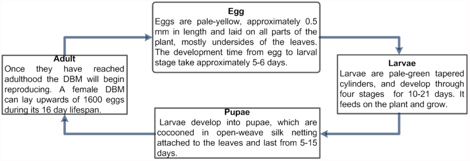
Figure 7 shows the four-stage life cycle of the diamondback moth. The total time it takes a diamondback moth to reach maturity is about 32 days. However, new generations appear 21 to 51 days apart, depending on conditions. 42
Egg. The diamondback moth lays eggs on the underside of a plant’s leaf (in groups of 1 to 3). It takes approximately 5–6 days for the eggs to reach maturity.
Larva. The larval stage can be split into four distinct steps that last 10–21 days, during which the larvae feed on the plant and grow. The time until maturity depends on environmental factors: temperature, food abundance, etc. The larval stage of the diamondback moth destroys leafy crops (cabbage, lettuce, etc.).
Pupa. This stage lasts 5–15 days.
Adulthood. On reaching adulthood, the diamondback moth will begin reproducing. A female diamondback moth can lay upwards of 1600 eggs during its 16 day lifespan.
Life cycle of diamondback moth.
Predator–prey relationships like this one are often modeled using discrete equations to determine population sizes at given times, using parameters derived from observations of real environments and shaped to fit the equations. Tonnanga et al. 43 used an analytical model to recreate the effect of introducing parasitoids (to determine the most efficient course of action to control the population). The Cell-DEVS model presented in this section is based on this model. The model uses seven different layers, each of which represents the behavior of different entities with limited interactions with each other and using a predetermined set of parameters.
Layer 1 (crop). The crop is assumed to have a fixed density (we do not model reproduction or death). Each plant will only allow a single egg to be laid on it, and it will only allow a single reproductive pair to perch upon it.
Layer 3 (pupa). This stage lasts 5 days, after which a mature diamondback moth will emerge if that location is empty; otherwise, it will die (representing an ecosystem with maximum support capacity).
Layers 4 and 5 (adult female and male diamondback moth). The adult moth has a lifespan of 16 days; moths can travel. The female moth searches for an empty plant, and on locating one, she stays there until fertilized. For the female moth to become fertilized, a male moth must occupy the same plant as the female for 1/10th of a day before leaving to find another mate. On fertilization, the female moth will leave the plant in search of an empty plant and a new mate. In nature, the male moth finds a female by detecting the aroma of the sex pheromone of the female moth.
Layers 6 and 7 (adult female or male parasitoid). These follow a similar search pattern to the diamondback moth, but the female parasitoid searches for a plant occupied with larvae.
To define the model using Cell-DEVS and to define it in CD++, we define two types of information in each cell: the age of the diamondback moth in the cell, and the direction of the next movement. The movement is done in two phases. First, if the value of the cell is 1, it changes its state to a random integer between 2 and 9. The cell value from 2 to 9 indicates the possible eight different directions of the next movement:
In the second phase, we decide whether a movement is feasible; in that case, it moves based on the possible directions determined. If not, it changes to 1, and it determines a new direction according to phase one, as follows:
The age of the cell is stored in the decimal position. For this model, one complete movement cycle is considered as 1/500 and 10 complete cycles are considered as one day, which is 0.02. An adult diamondback moth has a lifespan of 16 days, as mentioned earlier. Therefore, when the decimal position reaches 0.32, the lifetime of the diamondback moth is ending.
On finding an empty plant, the female moth remains in the cell. A similar approach is taken with the male moths, but the difference is that the male moths search for available mates. The female moth stays in an empty plant until fertilized. To fertilize the female moth, a male moth must occupy the same plant as the female moth for two cycles before leaving to find another mate. Finally, on reaching a count of 0.32, the insect will die.
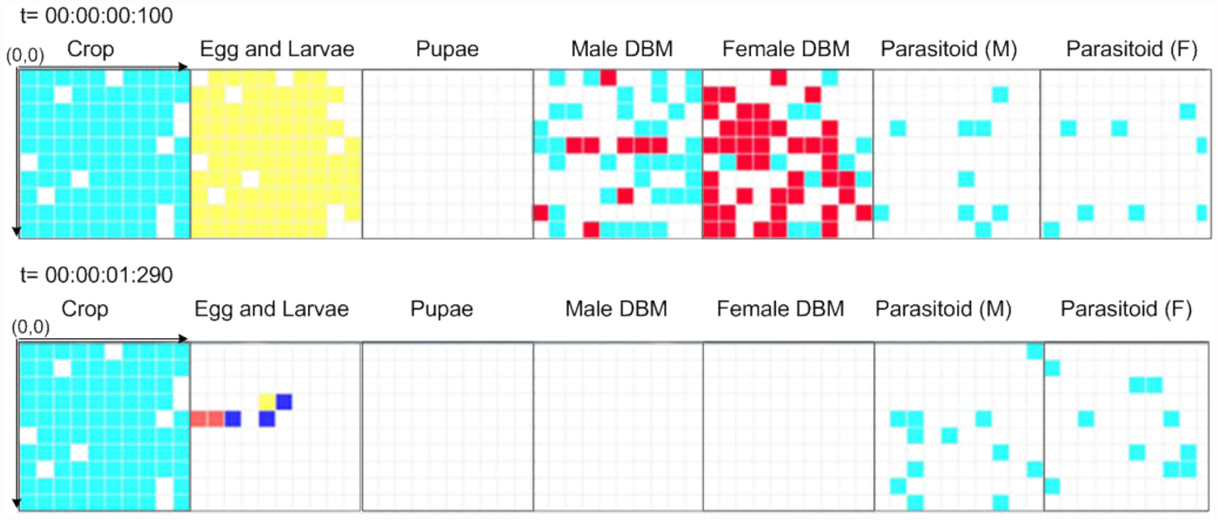
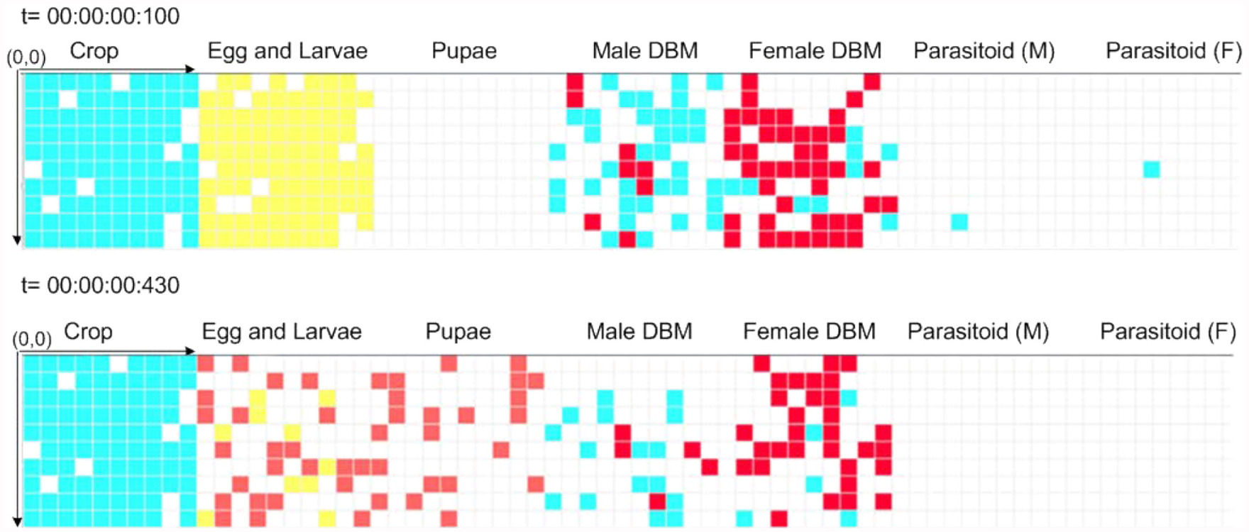
The different parameters in the model can be adjusted to model different biological events. In the following figures, we show three simulation scenarios: annihilation of the diamondback moth population, disappearance of parasitoids, and equilibrium. In the first scenario, the initial population of parasitoids is very high (and they are effective predators); therefore, they may destroy the population of diamondback moth. This is undesirable, since any return of the diamondback moth population would increase uncontrollably (the parasitoid population would have died as well, as it is not a native species). In the simulation results shown in Figure 8, the density of plants is set to 90%, the population density of diamondback moth is 50%, and the density of parasitoids is 10%. As we can see, the large initial population of parasitoids allows them to overrun the diamondback moth population, and it results in their complete destruction. Our second example (Figure 9) shows a case where the initial density of parasitoids was 2%, and, consequently, the population of the parasitoids disappears.
Test scenario: Annihilation.
Scenario for a low level of parasitoids.
The last example presented here (Figure 10) considers a case of equilibrium, in which the initial conditions of Figure 9 were not changed but the parasitoid population density was changed to be 3%.
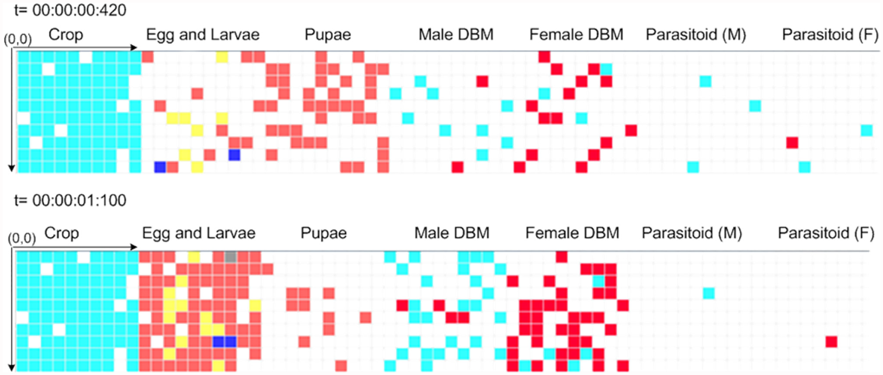
Equilibrium scenario.
The results show that the parasitoids managed to maintain a relative equilibrium for a notable length of time, supporting the idea that released parasitoids might be able to control the population size of the diamondback moth.
4. Integrated Cell-DEVS architecture for web-based simulation and GIS visualization
Integration of web services, modeling, and simulation, and of GIS with advanced visualization can increase the accessibility, representation, and understanding of simulation results of ecosystem systems. Many ecological simulation models have explored the potential of using GIS to store spatial data, to manipulate georeferenced information, to perform interactive analysis, and to display the results on maps.28,44,45
Integrating these subcomponents into one system has many advantages to support planning and decision making for ecosystem applications.36,44 In this section, we discuss the architecture of an integrated architecture of web service simulation using Cell-DEVS, GIS, and visualization, presented in Figure 11. The fundamental concept is to collect data from a GIS, model an application using Cell-DEVS, run simulations in a remote RISE server (which does not need installation efforts or software tailoring), and visualize simulation results (in this case, using Google Earth).
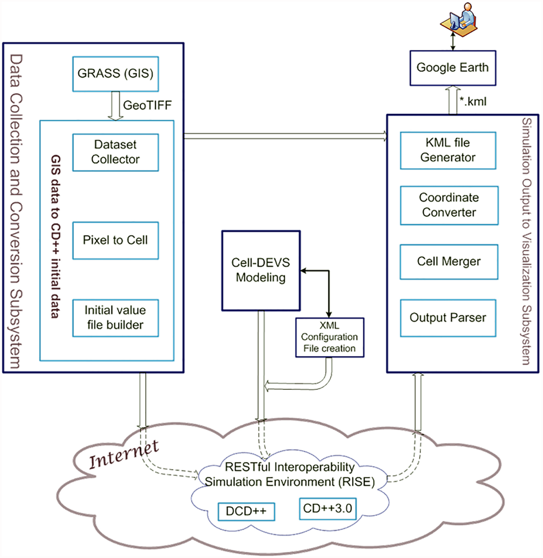
Integrated architecture of web-based simulation and visualization using Cell-DEVS.
The overall architecture includes four subsystems.
Data collection and conversion. This subsystem maps the information from real-world geo-ordinates to cell space ordinates; it converts the whole region under study into cells, and uses this information to initialize the simulation. It includes a dataset collector (for selecting georeferenced raster data from open standard GeoTIFF files), and a pixel-to-cell application (for converting it into the scale needed for Cell-DEVS models, like those presented in Section 3). The initial value file builder generates the initial states of cells and necessary attributes for the Cell-DEVS model.
Cell-DEVS modeling. This subsystem builds a Cell-DEVS environmental model according to the data collected. It defines the cell space size, neighborhood, and rules of the model behaviors using the CD++ modeling tool, following the ideas presented in Section 3.
Web service simulation. This subsystem runs Cell-DEVS models in RISE (remotely in the Cloud), and it gets the simulation results. Different simulation engines with CD++ variations are stored on the server and can be run remotely using RISE.
Visualization. This subsystem provides a visual depiction of the simulation results (in this case, using Google Earth). Once the simulation results are retrieved from RISE, the subsystem parses the simulation results, optimizes the cells, and converts the coordinate system using the cell merger and coordinate converter components for visualization. The subsystem generates a KML file (which can be imported, for instance into Google Earth), allowing the visualization of the simulated results on a customized layer impressed over the standard layers.
In the following sections, we will use a simple land use change model as a prototype to illustrate each step of the proposed integrated web service simulation architecture.
4.1. GIS data collection and conversion
This subsystem is responsible for extracting data from GIS, converting the target region into cells, and storing the required information into initial value files for the Cell-DEVS model. This section illustrates the procedure for GIS data collection and conversion in detail.
As we can see in Figure 11, the subsystem includes three modules: dataset collector, pixel-to-cell converter, and initial value file builder. Figure 12 shows the class diagram of the data collection and conversion subsystems. AbstractGeoReader implements the general logic of the data input, including two subclasses: MetaDataReader, responsible for fetching geographical references, and DataReader, responsible for obtaining data on each of the pixels. GeoTiffFileReader implements these methods to obtain information in GeoTIFF format. GRASSReader retrieves data through the GRASS API. GeoTiffFileReader implements these operations. Geoinfo stores geographic contextual data (coordinates and resolution) of the area. PixeltoCell approximates the most common value covered in a cell area that contains multiple pixels. Valwriter class generates the cell’s initial values.
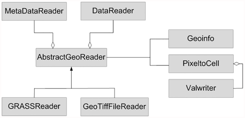
Class diagram of data collection and conversion subsystem.
As discussed in Wang and Wainer 36 and Zapatero et al., 37 these various components are needed because in GIS, as in GRASS, information of a specific area is organized as a collection of vector or raster or imagery data, and we need the data to be converted as initialization information for the CD++ simulator.
We import initial geographic information as raster or vector data in GeoTIFF format using the Geospatial Data Abstraction Library. We will show the process using a sample raster dataset from North Carolina, USA. This GeoTIFF file, provided by GRASS, is based on a dataset that offers raster, vector, LiDAR, and satellite data. We selected a raster dataset including geographic layers of land use, elevation, slope, aspect, watershed basins, and geology from this GeoTIFF. Raster datasets group different layers into bands containing common information. Each raster band contains the map size, the Geospatial Data Abstraction Library data types, and a color table for mapping color and land use type values, as shown in Figure 13. Each raster band consists of several blocks for efficient access; each block consists of several pixels. The basic idea is to look through the dataset to get pixel information. In Figure 13, the land use of the studied area has one raster band with four blocks, separated in total by 179 pixels × 165 pixels, and seven land use color types out of 24 types.
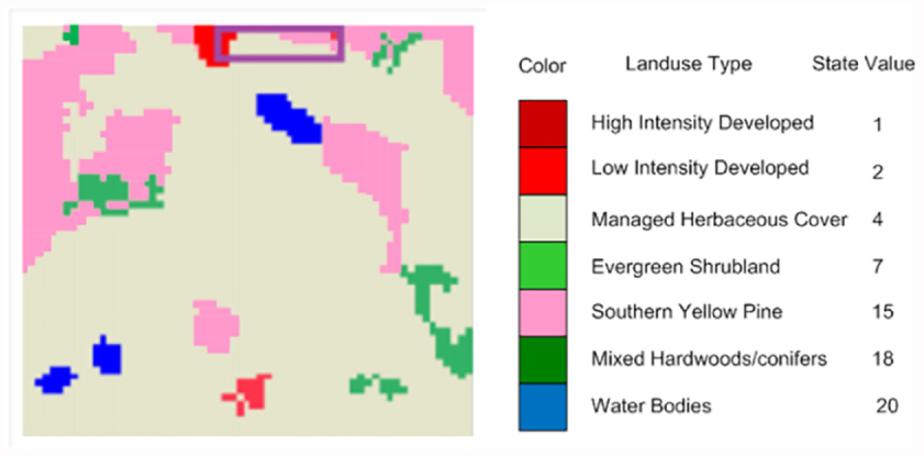
Studied area of “land use” map and corresponding states (Wang and Chen 2012).
The PixeltoCell converter reads the block data of the raster band, collects the color value of each pixel, and generates the initial value of the corresponding cell for the Cell-DEVS model. Ideally, each pixel could match an exact single cell, but this is not always the case. Indeed, usually a number of pixels are covered by a single cell, which is scaled with the minimum unit of a geographical map. In these cases, we use a queue for each cell, sort the pixels shown in this cell according to their state value, and choose the most common state value in the queue as the representative state value. Figure 14 shows an example for this case, in which the state value 7 appears twice, the state value 15 also appears two twice, the state value 1 appears once and the state value 20 appears four times. Therefore, 20 becomes the corresponding cell state value for the Cell-DEVS model. All these state values represent different colors in map, as discussed.
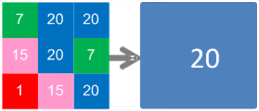
Approximate cell state value from a number of pixels.
After this approximation step, we obtain the initial values for the model of interest (in this case, a 20 × 20 initialization set for the land use). We store the required information into the initial information file, along with geographical contextual data, such as coordinates and the resolution of the area.
4.2. Web service simulation
As discussed earlier, the RISE middleware provides services over a number of resources or URIs, and these resources exchange synchronization information in the form of XML messages via HTTP methods (get, put, post, and delete). The URIs are organized hierarchically, with multiple instances of each template created simultaneously by different users, as shown in Figure 15. For example, the template “{userworkspace}” allows any number of a modeler’s workspaces to be created, separating the user’s experiments from each other. The “{servicetype}” template allows each modeler to select a simulation service, and to build experiments based on different environments. For instance, we have two types of “servicetype” of simulation engines. The “{framework}” template indicates that the modelers may create any number of experimental frameworks with any supported simulation environment, as shown in Figure 15. For example, typing “…/Bob/DCDpp/” in a web browser will return all of Bob’s resource experiments that use the DCDpp simulation engine.
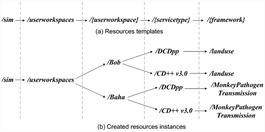
RISE URI templates with example instances.
RISE allows modelers to create experiments based on different simulation engines. In the current RISE environment, we have DCDpp for distributed simulation and CD++ v. 3.0 as the advanced CD++ version with multiple state variables and ports. The following XML configuration file shows information for a Cell-DEVS model. Each partition will run the simulation session in a dedicated CD++ engine, which is located in the belonging machine with the IP address and port specified in this document:
4.3. Visualization process
After retrieving the simulation results from RISE, we need to interpret the results. To do this, we need to transform them so that we can visualize them in a GIS or geospatial visualization system. The visualization of the results using a geospatial visualization system can enhance the communication of the results to domain experts as well as non-technical users, providing instantaneous access to layered information.
Figure 16 shows a class diagram of this visualization subsystem. We first need to parse the data generated by the simulator, preserving the output messages that represent state changes (LogParser). The output of the LogParser is stored by the supporting structure class Loginfo. Then CellMerger joins cells with the same state in adjacent areas, to reduce the amount of data to visualize. Next, CoordinateConvertor changes the coordinates in Loginfo so that it can be used by the visualization system. AbstactGeoWriter is an abstract class that provides an interface to the translation methods. Finally, KMLGenerator takes the Loginfo information and the georeferences, processes them, and generates a KML file with a timed representation of each simulated cell state change. The process consists of translating each output message into KML tags. Once the KML file is generated, it can be imported into Google Earth, allowing visualization of the simulation results.36,37
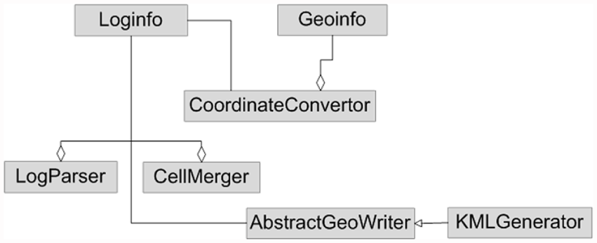
Class diagram visualization subsystem.
4.3.1 LogParser
The output messages store the change information of the cell values of the simulation results. This module parses the simulation results, preserving only the output messages and transferring them into the proper format defined in Loginfo. The format of the matched message is shown in Figure 17. The message always begins with Message Y followed by the timing and cell position information. The new state of the cell is transmitted and it is shown after the /out/ substring.

Output message format of CD++ simulation.
4.3.2 CellMerger
To describe the geography information of each cell, we use four positions in each parsed message; so we need to record the four coordinates for further operation. Each cell requires one <placemark> element in the KML. Moreover, if the size of the KML file increases, the rendering time will also increase when loading to Google Earth. Therefore, it is important to keep the number of KML elements as small as possible. CellMerger is responsible for solving this issue. The basic idea is to merge adjacent cells with the same value. An example is been shown in Figure 18; instead of using 16 place marks (Figure 18(a)) to represent every cell, CellMerger could merge the cells with the same value together, reducing the number of place marks to 4 (Figure 18(b)), and generate new polygons.
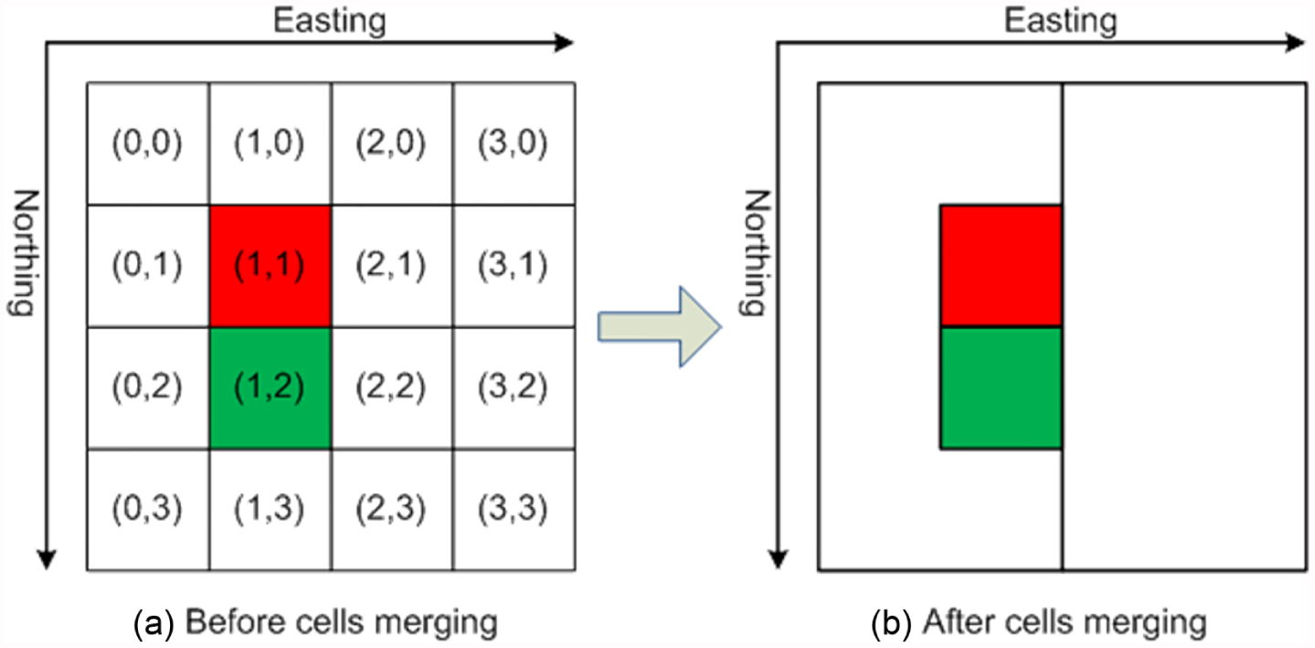
Merge cells with the same state value into polygons.
4.3.3 CoordinateConverter
As we know, environmental and ecological models are sensitive to georeferenced information. In our architecture, the initial data of the model are collected using GIS (GRASS) and geo.info stores the geographic information of the studied area, as we discussed earlier. The geo.info retrieved from GRASS uses the Lambert Conformal Conic Geography Project System. 35 The plane size is fixed by the coordinates of the upper left, lower left, upper right, and lower right corners. By contrast, Google Earth uses a reference system called the World Geodetic System 1984, which uses longitude and latitude pairs to define specific positions on Earth. Therefore, the information and initial parameters in geo.info have to be converted to longitude and latitude pairs of each cell to visualize the simulation results on Google Earth. In the implementation, each cell has four corners with positions of (east, north), as shown in Figure 19; after the cell-merging step, only the corner points of all the boundaries in a merged geometry must be known. 46
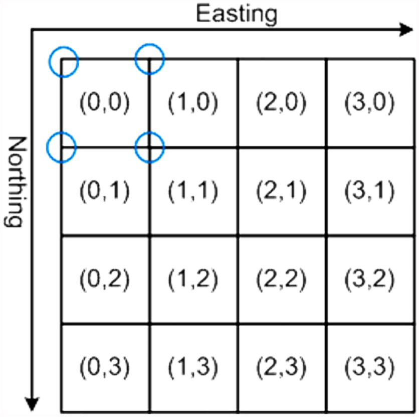
The square point of a cell.
4.3.4 KMLGenerator
Google Earth is a powerful visualization system supporting KML elements to display geographic data. KML is based on the XML standard, and uses the tags and its attributes to describe the geography information. In our implementation, we used a subset of the elements defined in KML, including <Document>, <Style>, <Folder>, <Placemark>, <Polygon>, and <Timestamp>. After knowing the information needed for each <Placemark> element (the coordinates of the merged polygon boundaries, the timestamp, etc.), we can generate a KML file. In the KML header, the state values and associated colors (defined in the Cell-DEVS model) are rewritten as polygons to paint each <Placemark> element. To define the body of the KML, each <Placemark> element of the merged cells will list all the coordinates of its polygons, and a <Timestamp> element will be inserted. Finally, the complete procedure generates the geographical area that emulates the simulation.
In Figure 20, line 1 is an XML header and line 2 a KML namespace declaration. Lines 3–24 describe the <Document>, which is our Cell-DEVS simulation. Within this, lines 5–7 define a style. We can define different colors for different cell states. Lines 9–21 represent the <Placemark> element, which depicts the cell region (square or polygon). Finally, line 22 defines the <Timestamp> element that indicates the <Placemark> timestamp.
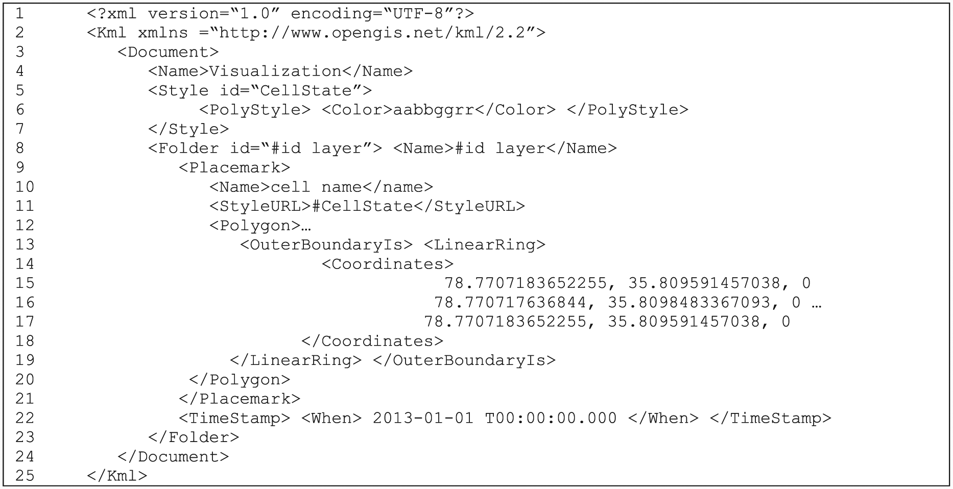
Sample KML file.
5. Case study: a monkey pathogen transmission model, simulation, GIS, and visualization
In Section 4, we discussed details of the integrated Cell-DEVS architecture for web-based simulation and GIS visualization. Here, we show a complete case study based on the transmission of a monkey pathogen, to demonstrate how to use our architecture. The model is designed using Cell-DEVS, essential geoinformation of the model is collected using GIS (GRASS), simulation is done in our web environment using CD++ and the RISE middleware, and, finally, we visualize the result in Google Earth.
An understanding of the pattern of pathogen transmission can play an important role in assessing potential disease control strategies to prevent outbreaks. We design the model based on Cell-DEVS to study a region of Bali, Indonesia, based on the work presented by Kennedy et al. 47 Macaques (a kind of monkey) on the island are known to carry a specific pathogen that is transmissible to neighboring macaques. Every monkey is able to host the pathogen; there are four different stages: susceptible, latent infection, symptomatic infection, and acquired immunity, as shown in Figure 21.
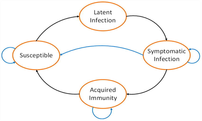
Pathogen transition stages.
Susceptible indicates that the macaque is vulnerable and can be infected. The period of latent infection is how long a macaque takes to become symptomatic after becoming infected by neighbor macaques that are in a state of infection or immunity. The period of symptomatic infection is the duration for which the macaque suffers from the disease. The period of acquired immunity is the amount of time a macaque is clear of a pathogen. In our model, we use the simplified state diagram shown in Figure 21. Pathogen transmission among macaques is affected by different properties, such as movement of the macaques, their sex, and the surrounding environment. The movement of the macaque has also been influenced by landscape features. For example, macaques move at random, but tend to pass through waterways less frequently than forests, and female monkeys are unable to leave their birth “temples,” which have been present in the forests of Bali for centuries. 47 Therefore, the probabilities of the movement associated with the landscape features.
The model we built uses three-dimensional cells to store different parts of the model. It includes five layers with five state variables for each cell. These are landscape, temple, movement, sex, and pathogen information, respectively, as shown in Figure 22.
Layer 1. This layer stores landscape information: these are coast-5 (the border of landscape), river-6, and forest-7.
Layer 2. This layer contains temple information: temple border-8.
Layer 3. This layer records all the movement-related information: 0 indicates that the current cell is not occupied while 1 means that the cell is occupied.
Layer 4. This layer keeps information about the macaque’s sex: 1 denotes male and 2 denotes female.
Layer 5. Finally, this layer stores all pathogen-related information: pathogens are shown with different states within the pathogen life cycle during movement.
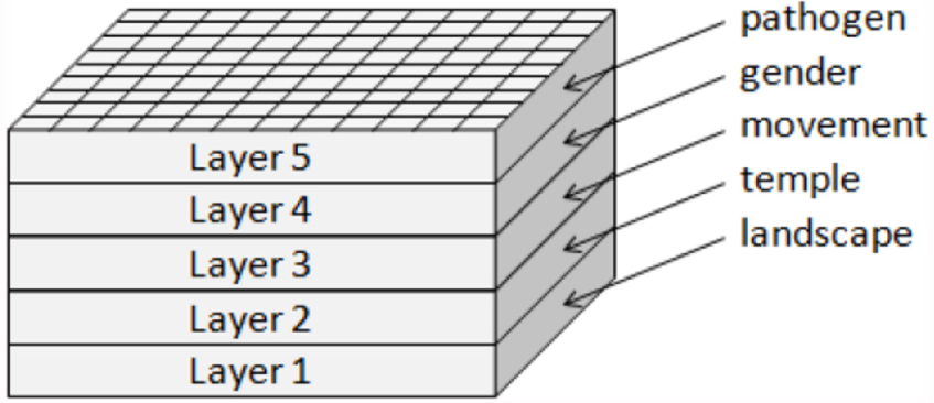
Different layers of the cell.
The expanded Moore neighborhood is used to model movement of the macaques. The basic neighborhood uses nine Moore neighbors ((−1, −1, 0) … (1, 1, 0)); to determine the movement, we also need to know the landscape and temple information, which are stored in (0, 0, −1) and (0, 0, −2). To realize random movement with different possibilities and temple constrains, the movement behavior is divided into four different phases: intent, choosing, constraint, and move. The state of each cell is defined by the values of its neighborhood cells following by a set of rules.
This model is sensitive to geoinformation of the site, such as river, coast and forest information of the island Bali, Indonesia, as well as some other parameters discussed before. The river and coast datasets for the region of Bali was collected using an open-source website, Cloudmade. 48 The forest dataset of the location is obtained from Carleton University’s Library GIS department. 49 These two datasets are combined using the GRASS GIS raster map calculator, as shown in Figure 23.
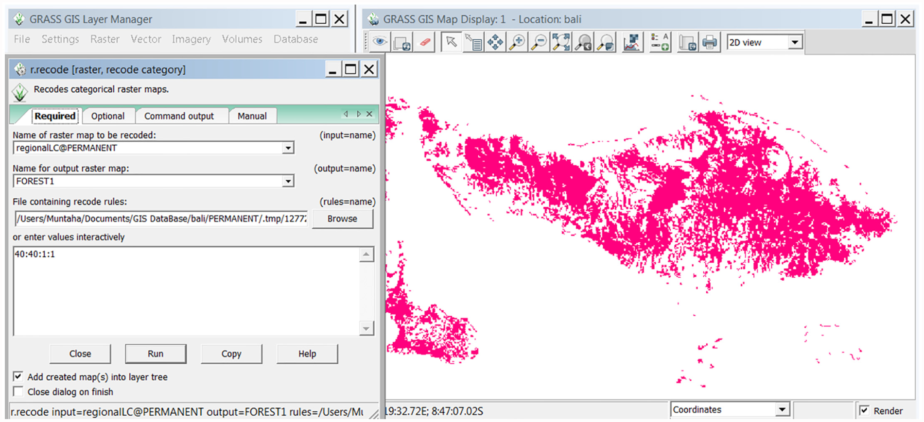
Raster map of Bali, Indonesia using GRASS GIS under the GNU General Public License, copyright 2017. 50
This map was used to obtain the landscape values of the model using our tool. The map is divided into a grid or cells and the landscape types are defined using different numbers. The initial map of Bali, with initial cell values for simulation, 50 is shown in Figure 24. After completion of data collection from GIS, we obtain the initial value file for simulation and visualization.
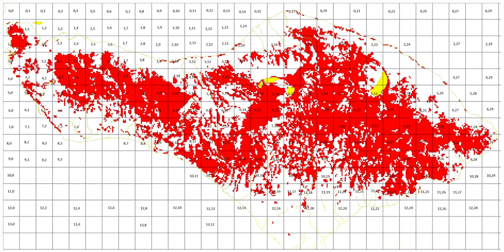
Initial cell values of Bali, Indonesia, after GIS data collection, using GRASS GIS under the GNU General Public License, copyright 2017. 50
To define the model using Cell-DEVS, we define the five layers discussed before. Each layer has its own behavior and cell components. The movement of the macaque and the transmission of the pathogen are defined using different rules in CD++. Figure 25 shows some sample rules used in different layers in the model.
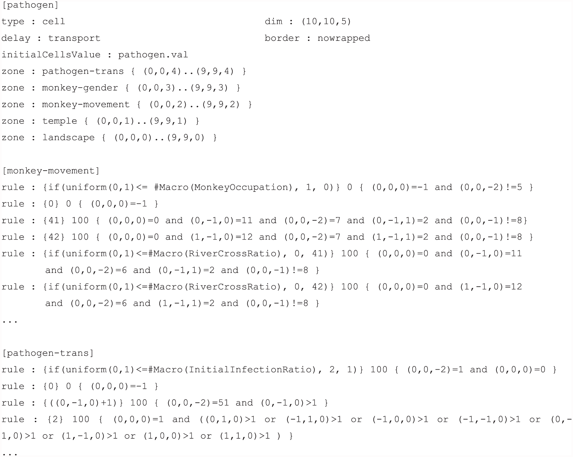
Model specification of macaque pathogen transmission.
The initial cell value is assigned through the file pathogen.val. We use the uniform() function to return a random number with uniform distribution within the interval. The macros MonkeyOccupation, RiverCrossRatio, and InitialInfectionRatio to determine the occupancy of macaques, the probability of river crossing ratio and the initial infection ratio.
This pathogen transmission model is simulated through the web-based simulation method over RISE middleware, as discussed in detail in Section 4. To use multi-state variables and multi-ports, we use CD++ v. 3.0 as a simulation engine within RISE middleware. The put method is used to create a new framework, …lopez/pathogen, using web-based distributed simulation engines under an authorized userworkspace in our RISE server. After this, the post method is used to upload the initial files (model configuration, initial values of each cell, Cell-DEVS model, etc.). Then the simulation is run using put to …lopez/pathogen/simulation and collect simulation results files from …/lopez/pathogen/results. After retrieving the simulation log file from RISE middleware, we can generate the simulation results in CD++ in two dimensions.
The model is tested under three different scenarios based on the various parameters, as we discussed earlier to show the effects of landscape, macaque occupancy, river crossing probability, sex, and initial infection ratio on transmission patterns, as shown in Figure 26. In each test, the right-most part of the figure shows the progression of pathogen with the movement of the macaque. Susceptible macaques are represented by blue cells, yellow cells represent latent infection, symptomatic infection is shown by red cells, and green cells indicate macaques with acquired immunity.
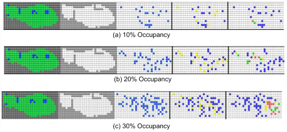
Simulation results of monkey pathogen transmission under different occupancies.
The simulation results can also visualized in Google Earth using the proposed architecture. We import the collected geoinformation and the log file retrieved from RISE into our GIS visualization tool to generate a KML output file, as discussed in Section 4. Finally, this KML file is loaded into Google Earth to visualize the model output. To verify the scalability of the architecture, we narrow the scale of our model to a small region. The whole of the island of Bali is shown in Figure 27 (left) and the small white square on the map is the region that we used to test the pathogen transmission model. Figure 27 (right) shows the visualization result with the zoomed-in region in Google Earth.
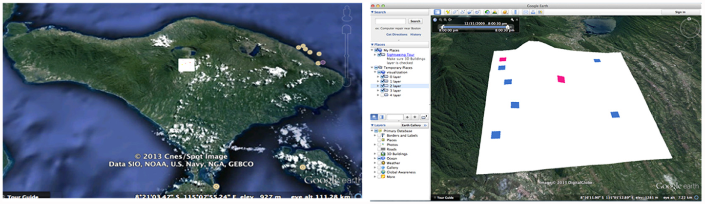
Bali map (left) and visualization results (right) from Google Earth (Map data: Google, DigitalGlobe). 50
6. Conclusions
In this paper, we proposed an integrated architecture for modeling, simulation, and visualization in the Web to study ecological applications. The proposed architecture integrates Cell-DEVS modeling, web-based simulation, and a geographical visualization system. We present the complete process of extracting information from GIS (GRASS), simulating the model remotely using RISE web-based middleware, and visualizing the result in Google Earth. Different case studies for various ecosystems have also been demonstrated using the proposed architecture. These case studies were used to test the proposed architecture and to demonstrate the benefits of the integration of Cell-DEVS modeling, web-based simulation, and GIS visualization.
The decoupling of Cell-DEVS modeling, web-based simulation, and geographical data handling modules makes this architecture highly scalable. Our future work could be directed as follows: (i) investigating efficient ways to integrate different modules in the proposed architecture; and (ii) incorporating cloud computing and providing simulation as a service.
Footnotes
Acknowledgements
The models presented have been developed by different students, including S. Wang, M. Lostracco, M. Younan, M. Zapatero, and M. Van Schyndel.
Funding
This work has been partially funded by NSERC.