
Abstract
Energy saving and environmental protection are important issues of today. Concerning the environmental and social need to increase the utilization of used products, this paper introduces two remanufacturing reverse logistics (RL) network models, namely, the open-loop model and the closed-loop model. In an open-loop RL system, used products are recovered by outside firms, while in a closed-loop RL system, they are returned to their original producers. The open-loop model features a location selection with two layers. For this model, a mixed-integer linear program (MILP) is built to minimize the total costs of the open-loop RL system, including the fixed cost, the freight between nodes, the operation cost of storage and remanufacturing centers, the penalty cost of unmet or remaining demand quantity, and the government-provided subsidy given to the enterprises that protect the environment. This MILP is solved using an adaptive genetic algorithm with MATLAB simulation. For a closed-loop RL network model, a special demand function considering the relationship between new and remanufactured products is developed. Remanufacturing rate, environmental awareness, service demand elasticity, value-added services, and their impacts on total profit of the closed-loop supply chain are analyzed. The closed-loop RL network model is proved effective through the analysis of a numerical example.
1. Introduction
One purpose of reverse logistics (RL) is to find appropriate methods that help dispose final waste products. By recycling the waste, enterprises can regain their value and raise resource utilization rates, while at the same time, environmental pollution and ecological destruction would be reduced. In an RL system, used products would undergo testing, warehousing, demolition, and remanufacturing. Since this system is directly affected by the location of nodes, the location of network nodes is important to remanufacturing enterprises. However, uncertainty would occur in an RL network due to the mistakes or delays in the supplier’s deliveries and the inexact forecasting demands. Because of the uncertainty of product recovery and demand, minimizing the total cost of an RL supply chain is more complex than that of a forward logistics supply chain.
Regarding today’s environmental sustainability issues, many scholars have studied RL to facilitate product recovery. Spengler et al. studied the recycling system in an open-loop supply chain in consideration of environmental and economic benefits using mixed-integer linear programming. 1 Fahimnia et al. proposed an optimization model for a closed-loop supply chain (CLSC) to promote supply chain decarbonization and a balanced carbon footprint. 2 Some scholars managed to construct an optimal reverse supply chain model by minimizing the total cost of a supply chain. For example, Amin and Zhang recognized multiple plants, collection centers, demand markets, and products in a CLSC and proposed a mixed-integer linear programming model to minimize the total cost. 3 Ene and Ozturk compared open-loop supply chains with CLSCs and proposed a mathematical model enabling a multi-stage and multi-period RL network to maximize its total profit. 4 Kannan et al. proposed a multi-echelon, multi-period, and multi-product CLSC network model to take back the used products in RL and applied a genetic algorithm (GA) to solve for a solution. 5 Yan built a mathematical model to study how the application of Internet of Things (IoT) influences the supply chain’s revenues. 6 Many researchers have studied the CLSC. For example, Ozceylan and Paksoy proposed an uncertain mixed-integer mathematical model for a CLSC, 7 which includes both forward and reverse flows with multiple periods and parts. Subulan et al. developed a mixed-integer linear program (MILP) for a closed-loop model, 8 which is meant for medium-term planning in a CLSC related to a conceptual product with remanufacturing option. In the proposed model, both forward and reverse flows are included, and two production alternatives are considered. Kim et al. presented a two-stage supply chain and used a case to demonstrate that the supply chain can influence both the risk of returnable transport item (RTI) stock-outs and the deterioration rate. 9 They also studied the relationship between RTI return lot size and the production lot size of finished products. Cannella et al. found that a CLSC outperforms a forward supply chain, 10 both in mono-echelon and multi-echelon structures and under both stationary and turbulent market demands. Furthermore, reducing remanufacturing lead-time and promoting information transparency may be crucial to improve CLSC dynamics. Zhou et al. suggested that higher return yield contributes to reduced bullwhip and inventory variance at the echelon level but for the CLSC as a whole the level of bullwhip may decrease as well as increase as it propagates along the supply chain. 11 Habibi et al. demonstrated that joint optimization of collection and disassembly with coordination between them improves the global performance of the reverse supply chain including lower total cost corresponding to the component demand satisfaction. 12 Kim et al. developed a deterministic mixed-integer optimization model and robust counterparts to cope with the uncertainty of recycled products and customer demand in the fashion industry. 13 They showed that a robust counterpart with a budget of uncertainty is equivalent to a robust counterpart with a box uncertainty under special conditions.
In the above research on remanufacturing CLSCs, the demand function of products is set in two ways: first, new and remanufactured products that are completely homogeneous and require only one demand function; second, new and remanufactured products that are different in quality and require two relative smaller demand functions. However, new and remanufactured products are closely related to each other although they seem different. For new and remanufactured products, whose brands and performances are basically identical, their demands functions might be the same. While, for those whose brands and performances differ from each other, consumers would consume either new or remanufactured products based on their incomes. In this situation, the demands of new and remanufactured products would influence each other. Thus, in this paper, a special demand function is built for new and remanufactured products.
As for solving approaches, heuristic methods are a hot spot for the problem, such as the GA, simulated annealing algorithm, ant colony algorithm, branch and bound algorithm, out-of-kilter method, purpose algorithm, and so on. An adaptive genetic algorithm (AGA), which is one of the heuristic methods, can solve nonlinear large-scale problems.
Concerning the location, network design, and layout of RL, the GA used in the previous research literature is basically the traditional GA, but this paper uses the improved AGA. Previous studies on RL mainly focus on one of the situations of open-loop supply chain or CLSC. In fact, these two situations are common. This paper will consider both open-loop supply chain and CLSC. Moreover, the government’s subsidy factor is considered in the economic cost model of an RL network. The government will provide an operating subsidy for recycling products to the enterprises participating in environmental protection.
The innovation of this paper is also reflected in taking sensitivity analysis of four parameters, including remanufacturing rate, environmental awareness, service demand elasticity, and value-added services, and their impacts on total profit obtained from the CLSC into consideration.
Many of the above studies aim to optimize open-loop supply chains or CLSCs by building a MILP model to compute their total cost and solve the models to obtain the minimum cost.
This paper introduces an open-loop RL network model, which means that in this RL system, used products will be recovered by outside firms rather than by original enterprises. Based on the above literature, an MILP model is developed to find the optimal locations of middle nodes in this open-loop RL network model to minimize its total cost using an AGA.
In addition to the open-loop RL network, this paper also studies the closed-loop RL network, which means in this RL network, used products are recovered by original enterprises. The closed-loop RL network only considers the RL part of a CLSC.
This paper is organized as follows, In Section 2, we design an open-loop remanufacturing RL network and evaluate the solution methods by using a problem instance, then the obtained results are given and analyzed. In Section 3, we design a closed loop remanufacturing RL network with new products and remanufactured products which have a link between each other but not the same products. Finally, Section 4 concludes the paper.
2. Open-loop RL network
2.1. Remanufacturing open-loop RL network
This section studies an open-loop RL network, taking used products such as e-waste and automobile parts into consideration. In an open-loop RL system, used products are recovered by outside firms. Agents or businesses collect used products from retail stores or recovery points. Then, those used products are delivered to remanufacturing centers after storage, detection, and demolition. Some parts that can be reused such as raw materials are delivered to remanufacturing centers, while useless parts are delivered to a landfill center for disposal. Then, remanufacturing centers would complete remanufacturing processes, after which recycled products are delivered to demand nodes, such as the enterprises that specialize in components manufacturing and extraction processing. In this network, the facilities of the middle layer include storage nodes, demolition nodes, and remanufacturing centers. For convenience, the storage node and the demolition node would be considered as one point. The location points of the problem are storage and demolition nodes and remanufacturing centers. Recycling products can be delivered from recovery nodes to storage and demolition nodes for processing, and then to remanufacturing centers when accumulated up to a certain amount.
There are two major problems to be tackled in this stage: first, finding the locations of these nodes; second, determining the scale of processing. The remanufacturing open-loop RL network is shown in Figure 1.
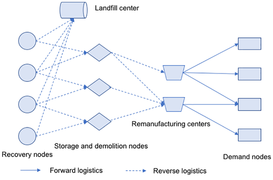
Remanufacturing open-loop reverse logistics network.
2.2. Assumptions of the remanufacturing open-loop RL network model
The assumptions of the remanufacturing open-loop RL network model are summarized as follows:
The target product is assumed as a single-type and single-cycle recycling electronic product.
The loss incurred during the recycling and material processing is not considered.
The recycling quantity and the demand quantity are considered stochastic vectors, and the expected values of these two stochastic vectors are taken as two uncertainty parameters.
Network construction and operation costs associated with the process are known. If there is unmet or remaining demand quantity, the penalty cost will be added.
Recycling facilities cannot exceed the processing power limit. Storage and demolition nodes and remanufacturing centers have capacity constraints.
Since it is easy to account for the final waste disposal costs, the costs of non-use waste would not be considered.
Based on the energy-saving intervention of the government, the subsidies given from government to enterprises that participate in environmental protection are considered.
2.3. Model construction
The open-loop logistics model adopts an MILP and considers three recycling processes: the freight from recovery nodes to storage and demolition nodes, the freight from storage and demolition nodes to remanufacturing centers, and the freight from remanufacturing centers to demand nodes. In this paper, the total cost of three recycling processes consists of the fixed cost, the operation cost of storage and demolition nodes and remanufacturing centers, and the penalty cost of unmet or remaining demand quantity. However, the government will provide a subsidy, which can be regarded as a negative cost, to enterprises that protect the environment. The model’s objective function is to minimize total cost.
2.3.1. Model parameters
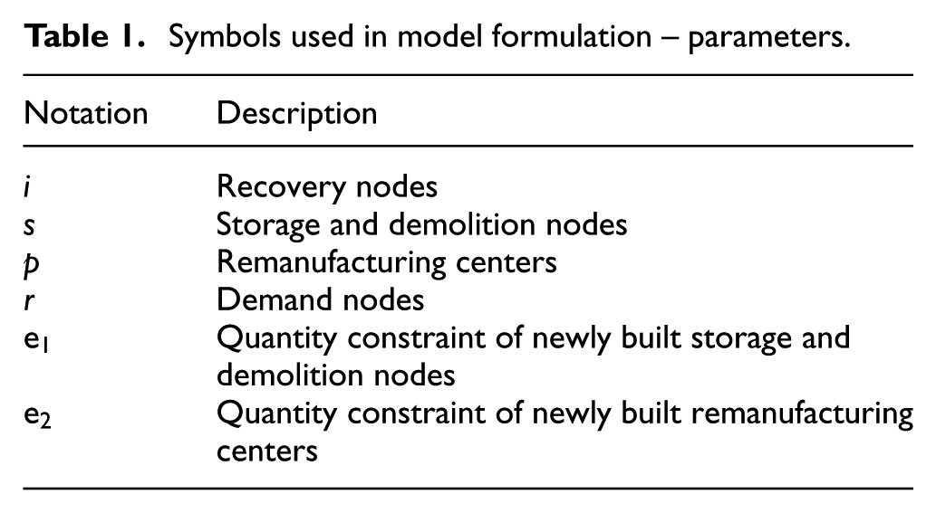
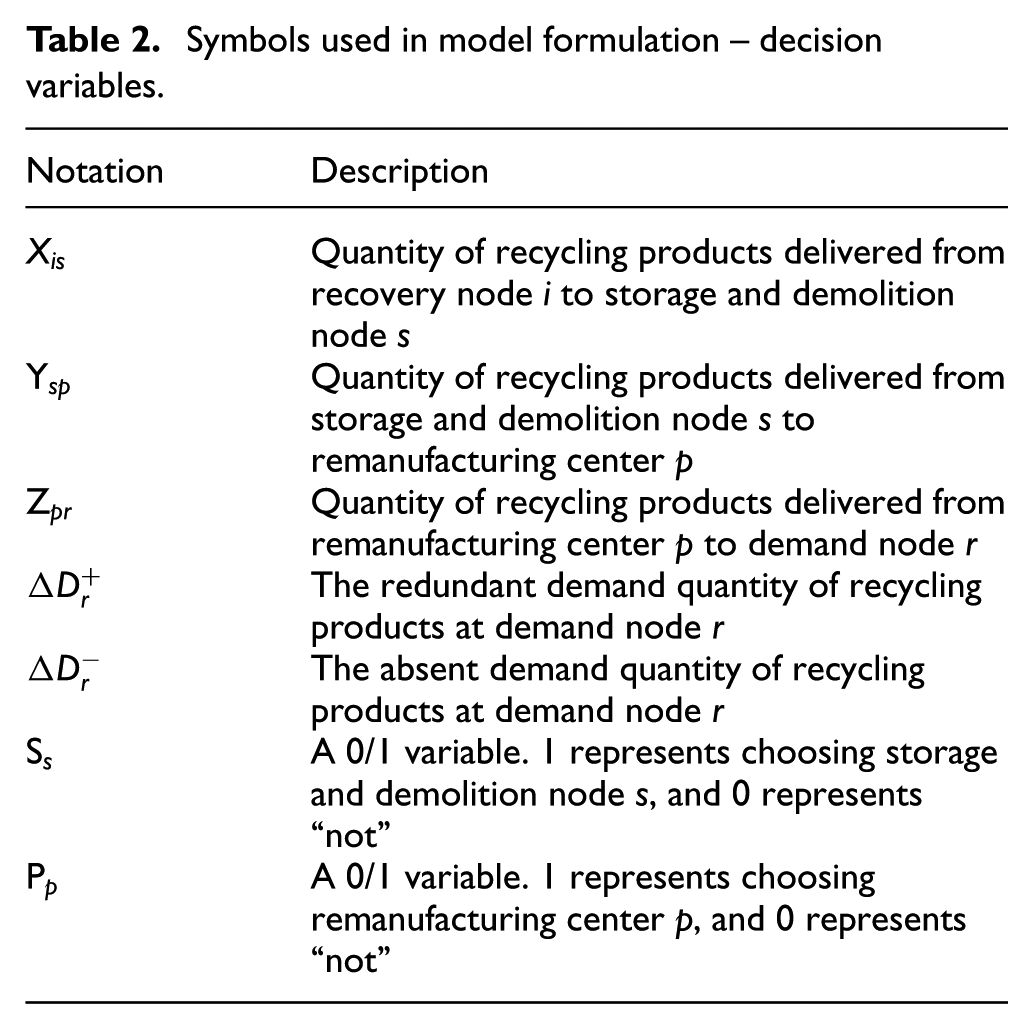
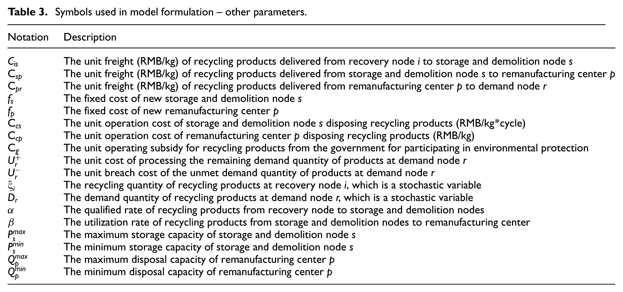
Parameters, decision variables, and other relative parameters used in the model and their descriptions are shown in Tables 1, 2, and 3, respectively.
Symbols used in model formulation – parameters.
Symbols used in model formulation – decision variables.
Symbols used in model formulation – other parameters.
2.3.2. Objective function construction
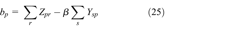
The model’s objective function is as follows:
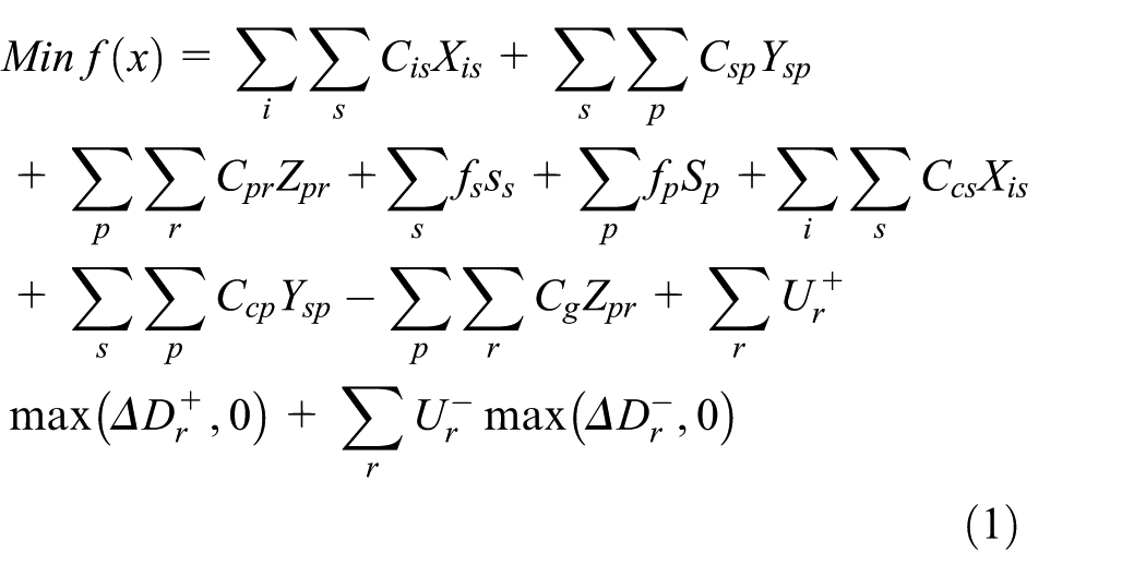
where
2.3.3. Constraint conditions
The following constraints are involved:
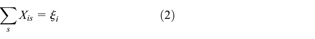
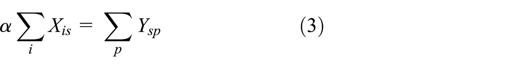
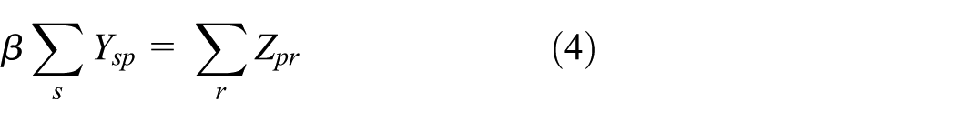
1. Flow equilibrium
2. Capacity constraints
3. Facility quantity constraints

4. Non-negative constraints

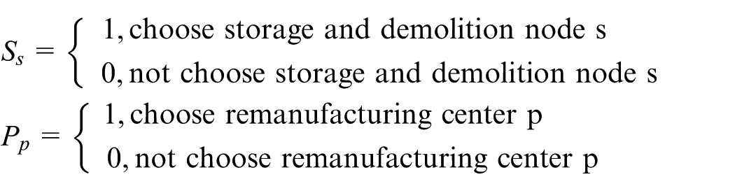
5. 0/1 variables

where
2.3.4. Model analysis
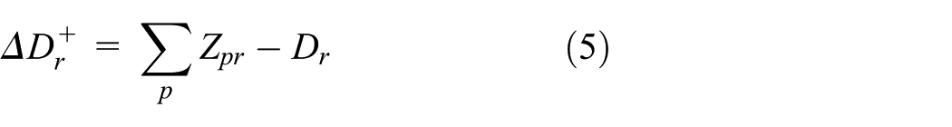
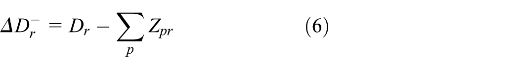
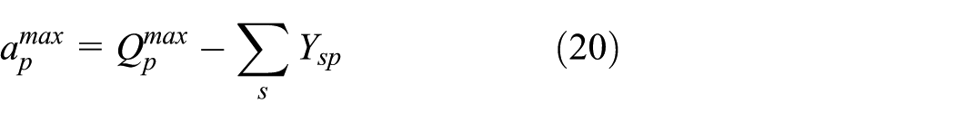
Among flow equilibrium, Equation (2) indicates that the output quantity of recycling products from recovery node i to other nodes is equivalent to the recovery quantity at recovery node i. Equation (3) shows that a certain proportion of the total quantity of products from each recovery node to storage and demolition nodes is equivalent to the total quantity of products from s produced in each remanufacturing center. Equation (4) demonstrates that a certain proportion of the total quantity of products from storage and demolition nodes to remanufacturing center p is equivalent to the total quantity of products sent from p to each demand node. Equation (5) represents the redundant quantity of demand node r, whereas Equation (6) represents the absent quantity of demand node r.
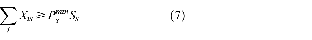
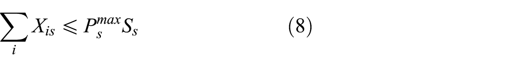
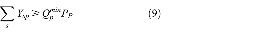
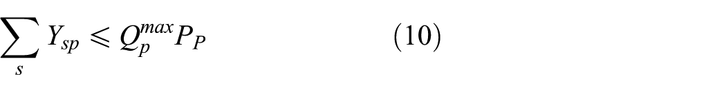
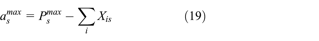
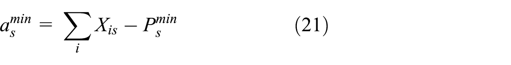
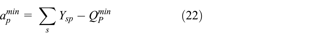
Among capacity constraints, Equations (7) and (8) indicate that the quantity of products running through storage and demolition nodes should not be less than the minimum amount of storage capacity and larger than the maximum. By the same token, Equations (9) and (10) indicate that the quantity of products running through remanufacturing centers should not be less than the minimum amount of disposal capacity and larger than the maximum.
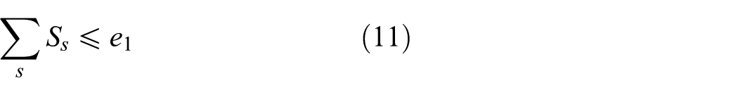
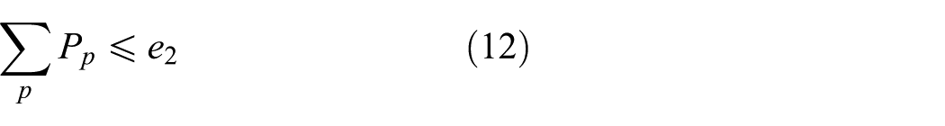
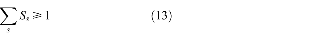
Among facilities quantity constraints, Equations (11) and (13) show that the number of new storage and demolition nodes should fit the number limit under the facility quantity constraints. Similarly, Equations (12) and (14) indicate that the number of new remanufacturing centers should fit the number limit.
2.4. Empirical analysis
2.4.1. Case description
This study conducts simulation by using MATLAB, which combines with the AGA to obtain a solution. In this case, S company, a large-scale household appliance company in China, will be analyzed. To simplify the research, this study will take a single-product, single-cycle situation as an example to show how to minimize the total cost in an open-loop RL system. Refrigerator recycling is chosen as an example. In this case, there are three recovery nodes, two demand nodes, three storage and demolition nodes, and two remanufacturing centers. We take three stochastic numbers generated by EXCEL by meeting the normal distribution N(180, 10) as three recycling quantities, which are 192, 181, and 176, respectively, and two stochastic numbers generated by EXCEL by meeting the normal distribution N(50, 5) as two demand quantities, which are 50 and 40, respectively. Here we assume that the demand quantities must be satisfied. The qualified rate
2.4.2. Converting constrained MILP to unconstrained MILP
A GA is employed to solve the MILP. The fitness values in the GA measure the optimization level of an individual in a population when they are verging on finding the optimal solution. The GA should not utilize outside information in the evolution of search, but only the fitness function is used for searching the better solution. Therefore, we should consider how to lift the constraints of the model.
To convert the constraint model into a non-constraint model, we use the penalty function method to punish the unfeasible solution. Constraints may be handled in this way, which is to increase the fitness value of strings that violate constraints by an amount proportional to the cost of violating the constraint. Thus, the constrained problem is transformed into an unconstrained one with a different penalized objective function.
The optimization model mentioned above can be expressed as follows:

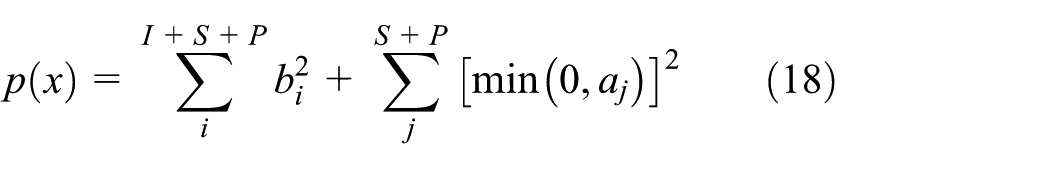

where
The penalty factor is
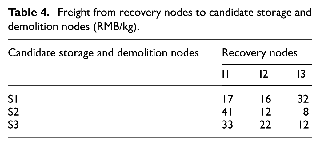
Freight from recovery nodes to candidate storage and demolition nodes (RMB/kg).
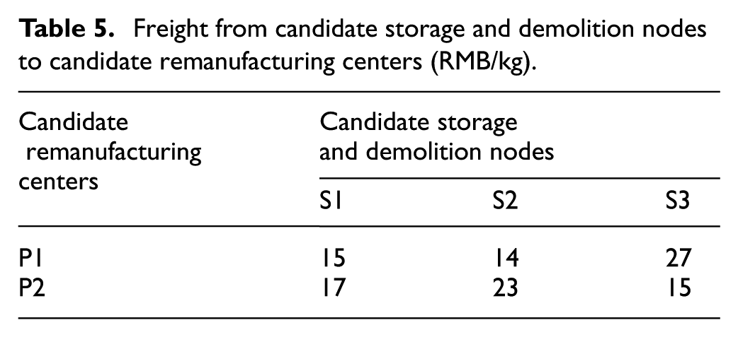
Freight from candidate storage and demolition nodes to candidate remanufacturing centers (RMB/kg).
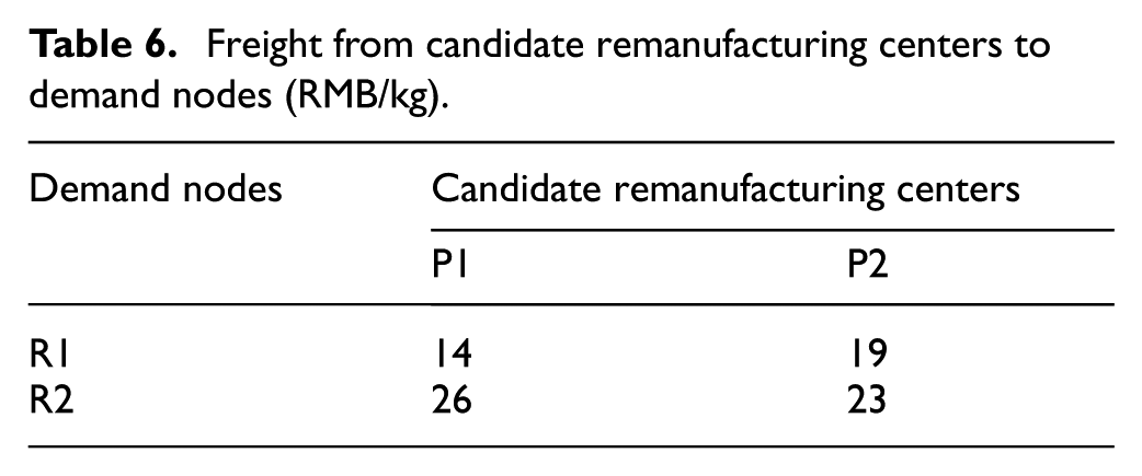
Freight from candidate remanufacturing centers to demand nodes (RMB/kg).
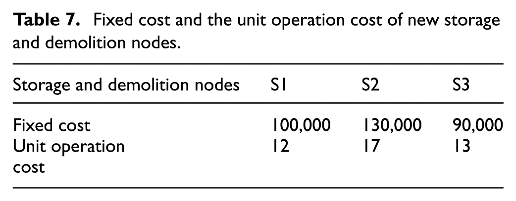
Fixed cost and the unit operation cost of new storage and demolition nodes.
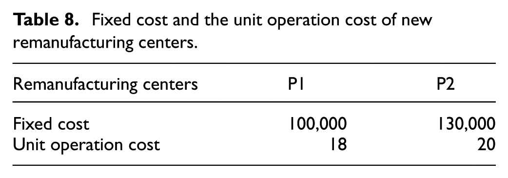
Fixed cost and the unit operation cost of new remanufacturing centers.
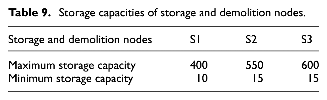
Storage capacities of storage and demolition nodes.
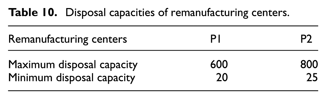
Disposal capacities of remanufacturing centers.
2.5. Solving the MILP by AGA based on MATLAB simulation
2.5.1. Comparison among different heuristic methods
Traditional optimization algorithms have strict requirements on objective functions or variables. Only when the objective functions satisfy certain conditions can the global optimal solution be guaranteed. Therefore, the traditional optimization algorithm is used to find the optimal solution of NP-complete problem. The computational time is unbearable or the computational time increases exponentially with the increase of the problem size because of the difficulty of the problem. Therefore, when solving large-scale combinatorial optimization problems, the traditional optimization algorithm is powerless.
As a network engineering problem, an RL system is a multi-objective, multi-constraint, multi-variable nonlinear programming problem. It is usually not feasible to solve the problem of facility location in RL by traditional optimization algorithms and the knowledge base/ rule base approach. Therefore, facing the problem of facility location in an RL network, we can solve it by heuristic intelligent optimization algorithm, because this method has fewer restrictions on the optimization design objective function and constraints.
Heuristic algorithms are the most appropriate methods that can be employed to solve the proposed MILP. There are some common heuristic methods, such as simulated annealing (SA), particle swarm optimization (PSO), ant colony optimization (ACO), and GA. Each algorithm has its own strengths and weaknesses. After comparing these algorithms, an AGA, an adaptive heuristic method, is chosen to solve this MILP.
SA traverses the search space by testing random mutations on an individual solution. It can only be ensured to converge to the global maximum with strict conditions, for example, enough high initial temperature. In addition, we must ensure that the temperature drops slowly so we can have enough samples under different temperatures.
PSO is a relatively simple prototype heuristic algorithm, compared with other bionic optimization algorithms. It has fewer parameters and is easier to get implemented. However, at the same time, it has lower accuracy and is easier to diverge. If the parameter, such as maximum speed, is too large, the particle swarm may miss the optimal solution and would not converge.
ACO can speed up its performance since it uses information positive feedback mechanism. However, at the same time, due to the influence of the positive feedback mechanism, ants will concentrate on several paths with higher concentrations of pheromone while neglecting the other paths, causing the algorithm to fall into the local optimal solution.
GA finds the optimal solution by simulating the mechanism of genetics in the natural world. It encodes the problem parameters into chromosomes for optimization; therefore, the algorithm is not limited by the function constraints. The search process starts with a collection of solutions rather than a single individual. With implicit parallel search features, it greatly reduces the possibility of an algorithm falling into a local optimal solution.
Thus, a GA is chosen to solve this MILP because of its great performance in avoiding local optimal solutions.
2.5.2. Brief description of the AGA
Deciding node locations in an open-loop remanufacturing RL system to minimize total cost is a process of optimization that considers all node locations as optimized regions and converts total cost into a fitness function through mathematical modeling. The fitness value determines individual survival. Individuals in a population consist of gene clusters with binary codes whose similar templates are called a “model.” In the early evolution of the GA, the model focuses on individuals with lower fitness. Thus, it is difficult for new outstanding individuals to generate due to low crossover and mutation rates. During the late evolution of the GA, the model focuses on individuals with high fitness. Thus, the algorithm would converge locally.
The GA requires improvement and these problems can be resolved in the following ways. First, the adaptive curve of crossover and mutation rate changes slowly in the average fitness of the population. Thus, individuals’ crossover and mutation rates which are close to the average fitness would be improved significantly. Second, retaining the outstanding individual model ensures that less optimal individuals retain the crossover and mutation rate. Therefore, the adaptive curve is smooth at the maximum fitness. This algorithm, called an AGA, was proposed by Srinivas and Patnaik. 14 In this paper, the AGA, an adaptive heuristic method, is chosen to solve this MILP.
A GA is a kind of simulated evolutionary algorithm which can effectively solve the function optimization problems. Numerous studies find that environment of parameters is essential to the quality of GA performance and results. The changes of parameters can affect the capabilities of function optimization. However, GA often uses fixed crossover probability and mutation probability in the practical applications, the crossover probability and mutation probability remain unchanged throughout the search process. Thus, it is difficult for a GA to converge to the global optimal solution in solving complex optimization problems. The AGA mainly focuses on adaptively designing the formulas of crossover and mutation probabilities. In addition, the crossover probability and mutation probability are adaptively designed with the changes of fitness values to preserve the best individual of the population and prevent premature.
2.5.3. AGA solving the MILP
The basic steps of the AGA are shown in Figure 2.
A mixed-code program with combination of binary encoding and float encoding is used to generate the initial group. In this paper, the constitution of a chromosome gene is designed and explained below. As shown in Table 11,
Calculate each individual fitness value in the group. Each fitness function takes the minimum value of the objective function.
The selection operator uses the tournament sort option. Although groups with the evolution have an increasingly number of good individuals, the best individual fitness may be destroyed in the current group due to the randomness of genetic manipulation, such as reproduction, crossover, and mutation. In general, the best individual fitness retains as many genes as possible into the next generation. Therefore, using the strategy of preserving the best ensures the survival of the fittest operation. In this paper, tournament sorting is used to obtain the next generation according to a specific fitness order, i.e., from smallest to largest.
The crossover uses a single-point crossover operator, whereas the mutation utilizes a single-point mutation operator. The crossover rate and the mutation rate adaptively change depending on individual fitness value. When the individual fitness value is lower than the average fitness value, a lower crossover rate and mutation rate are chosen so the optimal solution is protected to access the next generation. On the contrary, when the individual fitness value is higher than the average fitness value, a higher crossover rate and mutation rate are chosen so that the weak solution can be eliminated immediately. Thus, the self-adaptive crossover rate and mutation rate can provide a better solution, which is close to the true solution. Hence, the self-AGA maintains the diversity of groups while ensuring its convergence capability. The crossover rate and the mutation rate take a self-adaptive adjustment in accordance with the following formulas:
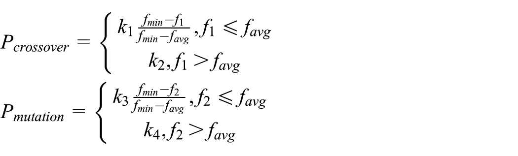
where
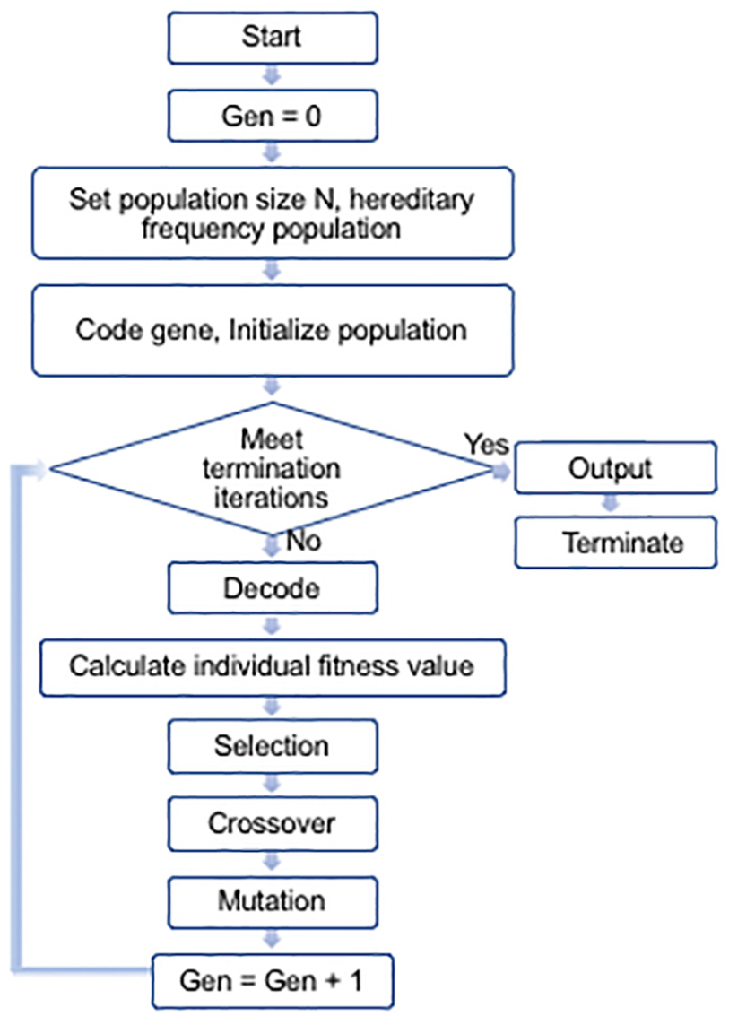
Steps of the adaptive genetic algorithm.
Constitution of a chromosome gene that includes 24 bits.

The AGA is an improvement on the traditional GA. A GA generates a new generation of individuals by using crossover operation which is essentially the process of genetic recombination. If the crossover probability is too large, the individuals of population update faster, and the individuals with high fitness values will soon be destroyed, which means the fine mode will soon be destroyed. If the crossover probability is too small, genetic recombinant will be reduced, ultimately leading to searching stagnation, and the GA does not converge. Mutation operation is essentially the disturbance of population mode in a GA and mutation operation can increase the diversity of the population. But if the mutation probability is too small, it will be difficult to produce a new model, if the mutation probability is too large, then the search will be more random. The crossover probability and mutation probability do not remain fixed in the AGA, and it greatly improves the convergence accuracy and rate of GA by adjusting adaptively genetic parameters. 15
The main parameters in the GA are the population size N, the crossover probability 1 1 1 0 1 17 90 100 28 67 71 56 91 34 0 32 0 63 0 24 0 0 1 69
If the maximum evolutional generation (Gen) is reached or error condition is satisfied, the algorithm must be stopped. The curves of the fitness value in every generation are shown in Figure 3. We can see that the fitness value converges to the optimal solution and remain basically constant after evolving only 32 generations.
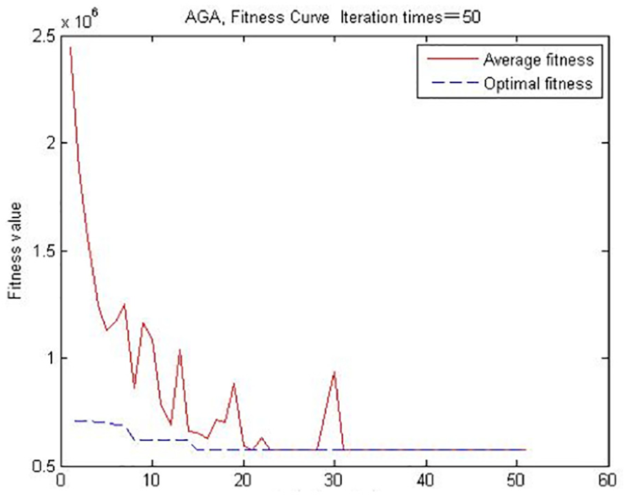
Fitness curve of the AGA.
As shown in Figure 3, the result indicates that the best chromosome gene comes out soon, passes to the next generation and is retained until the end of the iteration because adaptive and tournament sort options are used for accelerating convergence. Because of the crossover and mutation options, the curve shows a period of fluctuation. If the model scale is larger, it may require a certain amount of iteration to obtain the optimal solution.
The AGA shows a better performance that adapts surroundings in the optimization process, the convergence rate of AGA is significantly better, and AGA can find the global optimum. Crossover probability and mutation probability are no longer fixed in the AGA and the two important parameters can change with the values of fitness in the evolutionary process.
3. Closed-loop RL network
3.1. Remanufacturing closed-loop RL network
In this section, a remanufacturing closed-loop RL model is built based on the assumption that a two-step CLSC comprises a single manufacturer and a single retailer. The manufacturer produces both new and remanufactured products and sells them to the retailer; the retailer then sells these products to the consumers. Meanwhile, the retailer would recover waste products from consumers and sell them to the manufacturer for recycling. In this process, the residual value of the waste products
This paper applied the model under the condition in which all relevant information is known to all parties involved. New and remanufactured products are more closely related, but they are not the same products. Moreover, they are completely unrelated products, although their brand and performance are basically the same.
The remanufacturing closed-loop RL network is shown in Figure 4.
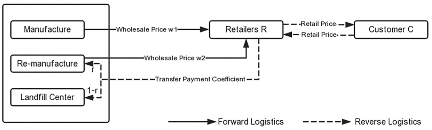
The remanufacturing closed loop reverse logistics network.
3.2. Assumptions of the remanufacturing closed-loop RL network model
The assumptions of the remanufacturing closed-loop RL are summarized as follows:
The model is a single-channel CLSC, i.e., the manufacturer recycles the waste products from the retailer.
The manufacturer can make new products and remake waste products at the same time.
Manufactured and remanufactured products are sold in the same market.
Customers have different preferences in the market, and they have no bargaining power.
New and remanufactured products differ from each other, but they are not completely different and they are linked to each other. Customers can choose different products based on their needs.
The demand curve of the retailer is a downward-sloping linear function.
The manufacturer is the core business in the CLSC and the leader of Stackelberg game; it has enough influence on the retailer who, in turn, serves as the follower.
The information between manufacturers and retailers are symmetrical and complete, and the decision making under manufacturers and retailers are completely open and transparent.
The manufacturer has sufficient production capacity to meet market demand, and the production cycle is very short. In other words, it is impossible to reach an “out of stock” situation in this system.
After market regulation, the amount of recycling waste products times the remanufacturing rate is
The number of retailer-recovered products is dependent on the manufacturer’s needs.
3.3. Special demand function construction
3.3.1. Model parameters
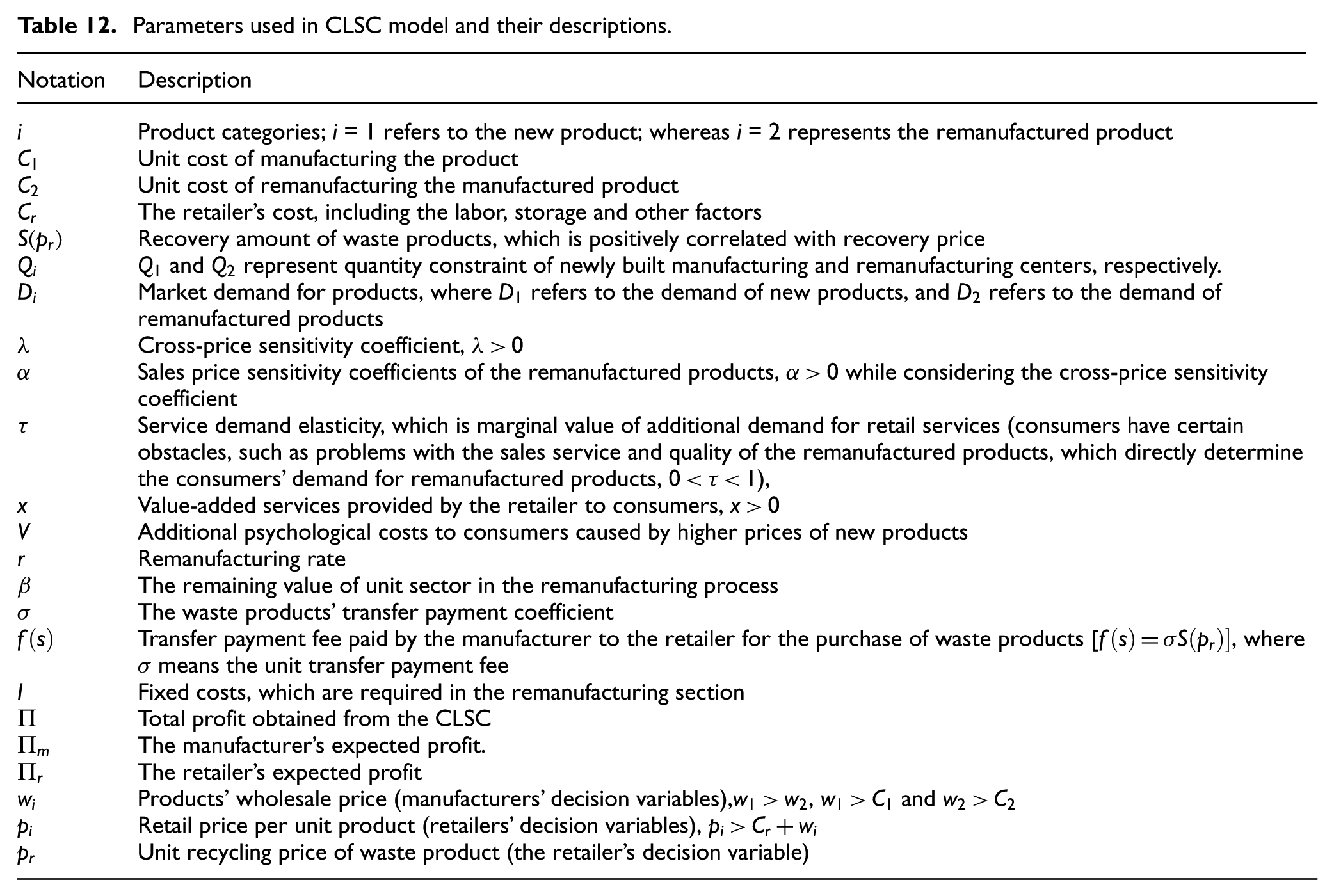
Parameters used in CLSC model and their descriptions are shown in Table 12.
Parameters used in CLSC model and their descriptions.
3.3.2. Building demand functions
By Bertrand game, when two products have common characteristics but cannot completely replace each other (i.e., their prices are not the same), the product with higher cost does not have to be off the shelf completely. Although these products are competitors, they have correlations, for example, they are made by one manufacturer; hence the brand, functions, and other factors are almost the same. They are distinct from other products which have different qualities. Considering some external factors such as retailers’ service and consumers’ psychology, two special demand functions of new and remanufactured products are developed as follows:


where
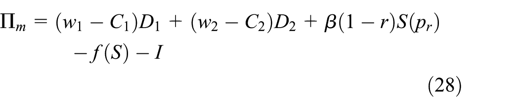
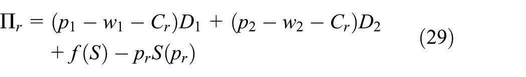
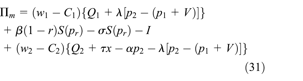
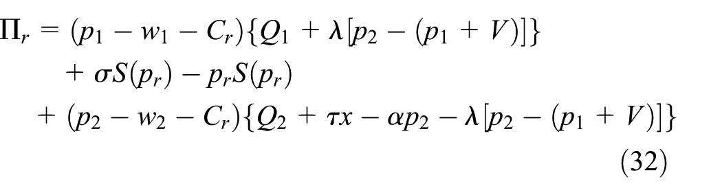
3.3.3. Building profit functions
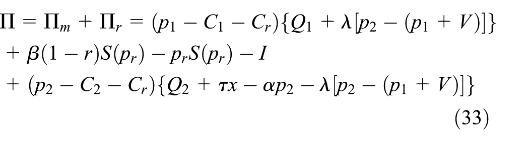
The manufacturer’s gross profit consists of the sales profit of new and remanufactured products and the residual value of the products that cannot be remanufactured. The costs include the transfer payments to purchase waste products and the fixed costs. By contrast, the retailer’s gross profit comes from new and remanufactured products sold to consumers and the profit gained from the recycling process. The cost is the recovery cost. The profit functions are as follows:
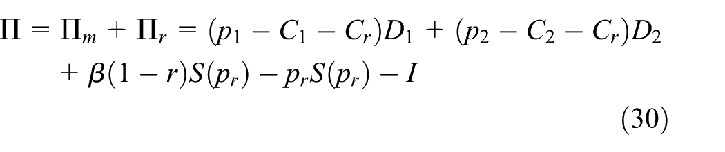
Then, we have
To ensure that the problem is significant, the variable parameters are assumed to satisfy the formula given by

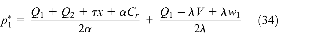
3.3.4. Gaining the optimal profits based on a Stackelberg model
The manufacturer and the retailer make decisions independently. Combining the dynamic programming approach and the backward induction approach of the dynamic games, we study the optimal policy of the manufacturer and the retailer in the background of remanufacturing closed-loop RL network. First, according to market demand
As the manufacturer’s product wholesale price
After integrating these equations into the manufacturer’s expected profit function
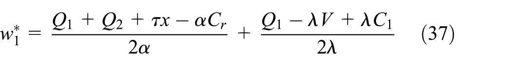
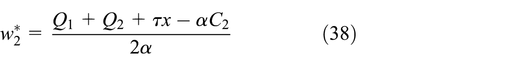
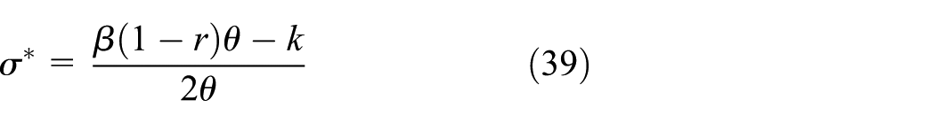
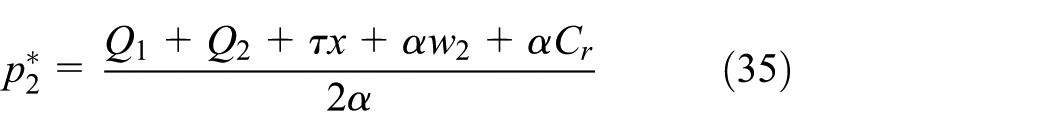
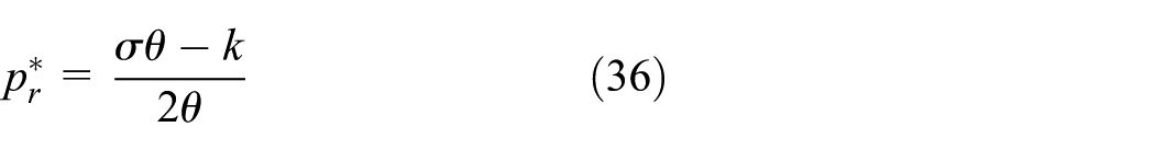
Then, substituting Equations (37), (38), and (39) into Equations (34), (35), and (36), respectively, we obtain the following:
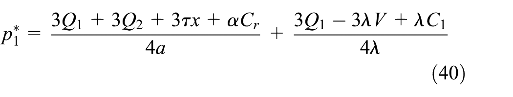
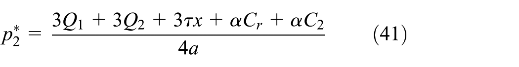
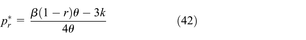
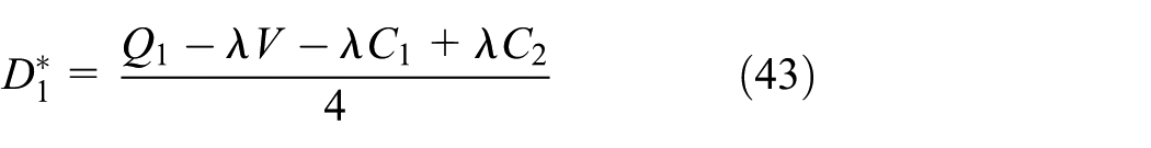
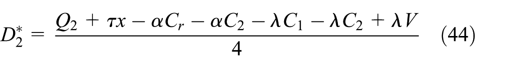
Taking Equations (40) and (41) into the demand functions of Equations (26) and (27), we obtain the optimal demand of new and remanufactured products as follows:
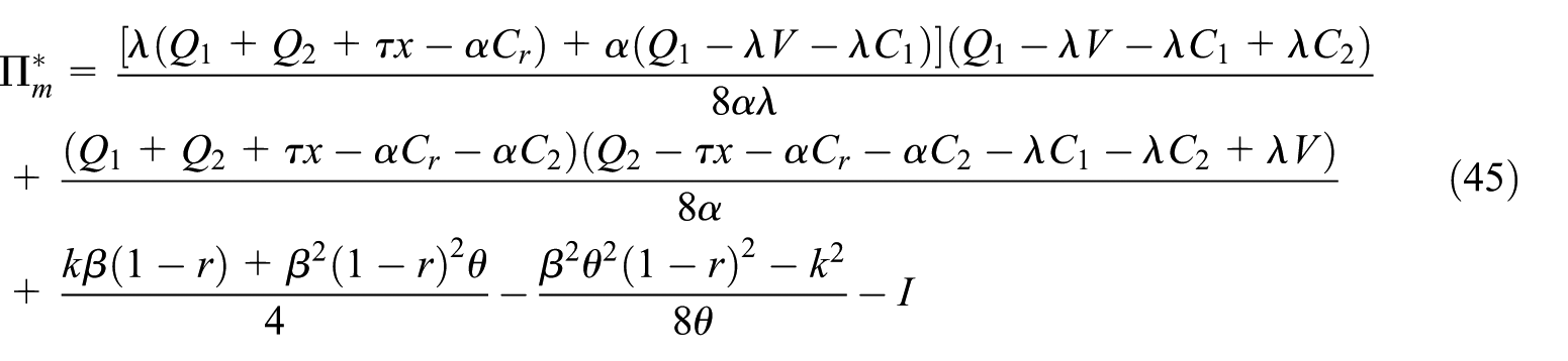
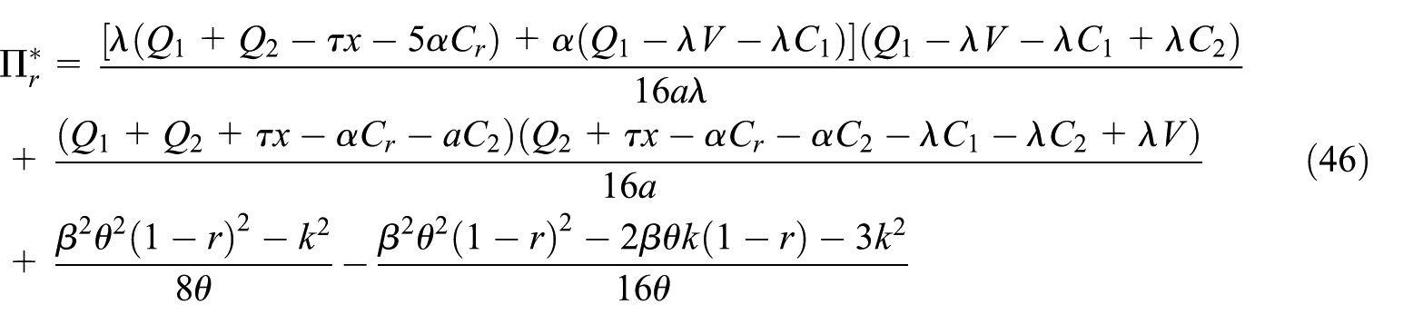
The optimal profits are expressed as follows:
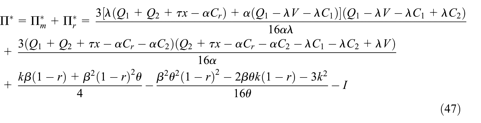
3.4. Solution and analysis
To illustrate the effectiveness of the model, numerical example is analyzed to study the effects of various parameters on profits, namely, the effects of
1. The relationship between remanufacturing rate r and the optimal profit
Supposing that
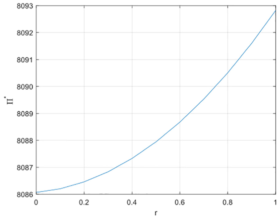
The relationship between
Conclusion 1: Remanufacturing rate r is a quadratic polynomial positively correlated with the total profit
2. The relationship between environmental awareness k and the optimal profit
Supposing that remanufacturing rate
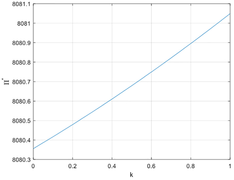
The relationship between k and
Conclusion 2: When environmental awareness k is strengthened, it can increase total profit of the supply chain. Previous theoretical analysis shows that the strengthening of public awareness of environmental protection increases the amount of recycling waste products and reduces the recovery cost of manufacturers at the same time. It benefits both the manufacturers and retailers. Hence, in terms of social benefits, enhancing public awareness contributes to the protection of the environment.
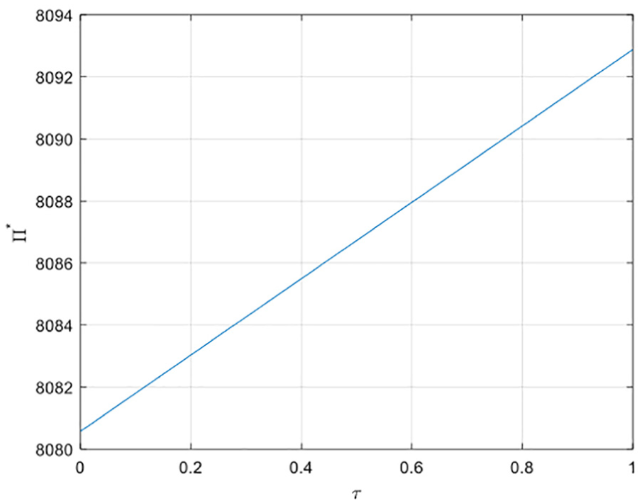
3. The relationship between service demand elasticity
Setting
4. The relationship between value-added services
The relationship between
Supposing that
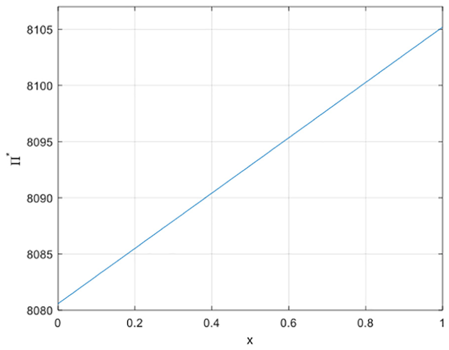
The relationship between x and
Conclusion 3: Both service demand elasticity
5. Sensitivity analysis of four parameters such as remanufacturing rate, environmental awareness, service demand elasticity, and value-added services and their comparisons of contribution to the optimal profit of supply chain
By drawing Figure 9 from Figure 5 to Figure 8 according to the same coordinate scale. We found that improving value-added services x has the greatest effect on the total profit of the supply chain, followed by service demand elasticity
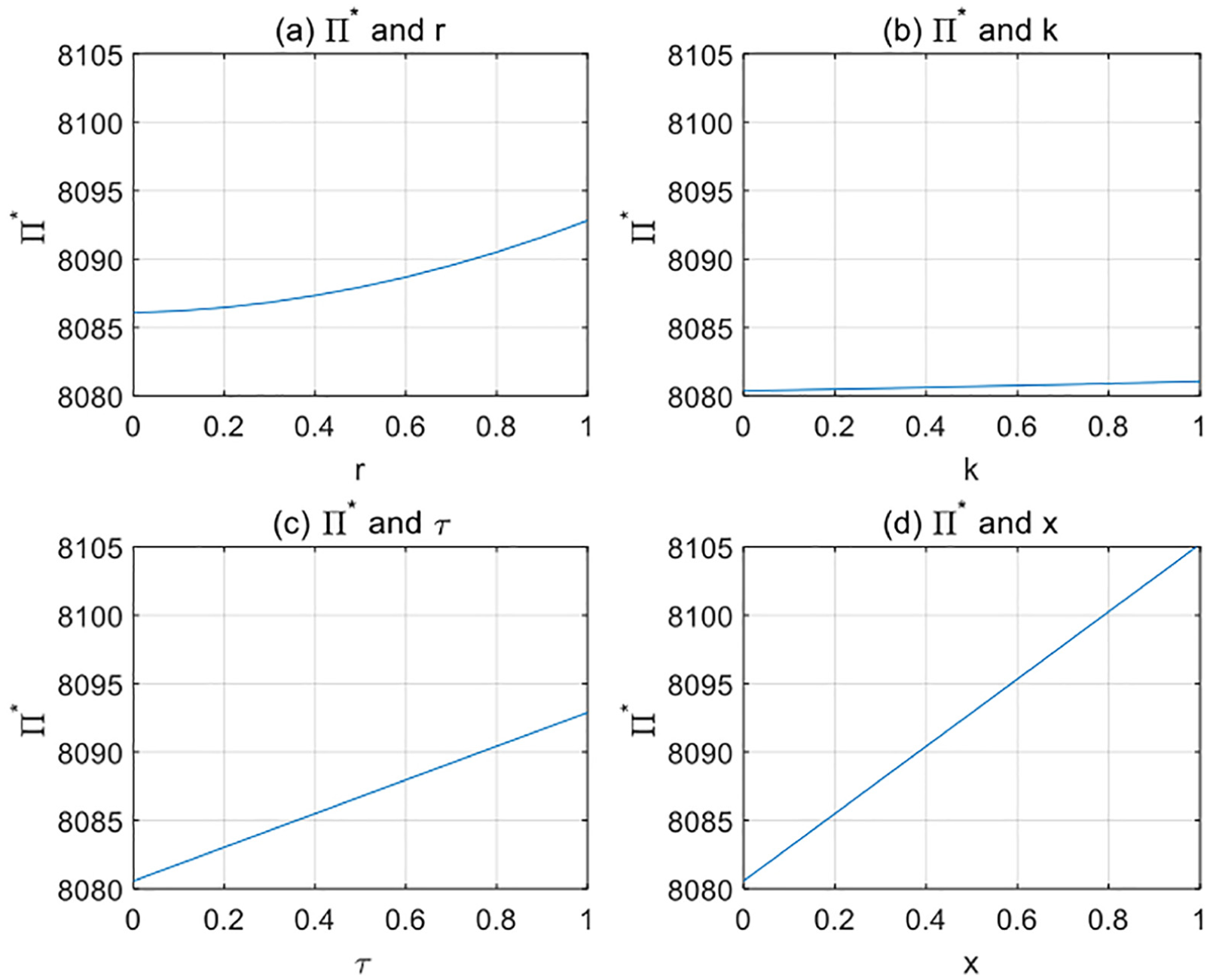
Sensitivity analysis of remanufacturing rate r, environmental awareness k, service demand elasticity
4. Conclusions
The location of middle nodes plays an important role in the recycling process of a reverse logistics (RL) system and it would affect the economic benefits to the enterprises undertaking such operations. In this paper, an open-loop remanufacturing RL network model is designed and a MILP is constructed to optimize the open-loop model by minimizing its total cost. The constrained MILP is converted into the unconstrained MILP with penalty function method and an AGA is provided to solve the MILP. This algorithm gives a faster convergence and thus would become useful to solve the open-loop model and find its optimal locations to minimize its costs. Given an example with result analysis, the feasibility of applying AGA on the RL network model is verified. This model can be used in the industry and helps logistics enterprises to make decisions that maximize their profits. It also encourages more enterprises to recycle products to protect the environment.
In addition to proposing an open-loop remanufacturing RL model, considering the relationship between new and remanufactured products, a closed-loop remanufacturing RL network model is designed. Many previous closed-loop models are built based on the assumptions that the demands of new and remanufactured products can be considered independent of each other because the performances and qualities of new and remanufactured products are the same for the same brand. However, this might not always be true. This paper considers the situation in which for different brands, the demands of new and remanufactured products might differ based on the prices and performances of their products. For example, different brands would have different environmental awareness and different service demand elasticity, which result to different optimal profits of the supply chain. To illustrate the effectiveness of this model, a numerical example is analyzed to study the effects of various parameters on profits. The results show that improving value-added services x has the greatest effect on the total profit of the supply chain, followed by service demand elasticity
We believe that further work can be done along several following research directions:
A more efficient intelligent algorithm will be designed to solve the model and is compared with the existing intelligent algorithm to get closer to the true solution;
The implementation of remanufacturing RL system involves the coordination of various logistics links between facilities, so it is necessary to carry out integrated research on logistics network design, inventory control, vehicle routing and production planning;
The problem of RL network design under uncertain time, quantity and quality of waste products recovery should be considered comprehensively.
Footnotes
Funding
This work was supported by the National Natural Science Foundation of China (grant number 71871098), the Natural Science Foundation of Guangdong Province (grant number 2017A030313415), the Humanities and Social Sciences Research Planning Fund Project of the Ministry of Education (grant number 18YJA630127), and Fundamental Research Funds for the Central Universities (grant number 2018YBXMPY19).