A modeling framework for the application of multi-paradigm simulation methods

Abstract

Decisions about modeling and simulation (M&S) of real-world systems need to be evaluated prior to implementation. Discrete Event, System Dynamics, and Agent Based are three different modeling and simulation approaches widely applied to enhance decision-making of M&S of these systems. Combining and/or integrating these methods can provide solutions to a plethora of systems’ problems. However, current solutions and frameworks do not provide guidance for selecting and deploying M&S models. Hence, the aim of this work is to present a generic modeling framework for combining and/or integrating Discrete Event, System Dynamics, and Agent Based simulation approaches. The framework is termed multi-paradigm modeling framework (MPMF). In this paper, we describe the research methodology that was followed for the development of MPMF, the different phases of MPMF, and the generic relationships of forming and deploying multi-paradigm simulation models. Then we evaluate the framework by using it for the implementation of a universal task analysis simulation model (UTASiMo). The MPMF provided guidance on what methods need to be incorporated into the UTASiMo models, what information is exchanged among those models, and how these models are connected and interact with each other.

Keywords

Agent Based Discrete Event simulation hybrid simulation System Dynamics modeling and simulation multi-paradigm modeling framework MPMF UTASiMo

1. Introduction

The need to evaluate decisions in real-world systems prior to implementation is well recognized in the literature.^1–4 Modeling and simulation (M&S) methods and, more specifically, Discrete Event (DE), System Dynamics (SD), and Agent Based (AB) approaches are widely applied as decision support tools to provide solutions to a plethora of system problems.^5–8

Most real-world problems refer to both continuous and discrete structures at the same time.⁹ In such situations, applying only discrete modeling approaches can significantly increase a model’s complexity, while using only continuous approaches fails to represent individuality.¹⁰ Moreover, traditional stand-alone M&S approaches can face serious challenges to represent the overall multidimensional nature of a system as a “whole”^{7, 11} and often emphasize more on a particular level of abstraction by tackling a specific set of modeling questions.¹² On the other hand, a multi-paradigm M&S approach allows the generation of simulations that may be interoperable and can capture interactions among elements at different abstraction levels by addressing a larger range of modeling questions and representing a variety of problem situations and applications.¹³ They also provide the modeler with a broader flexibility to represent more complex problems⁹ and reduce the amount of computational effort required to obtain acceptable solutions.¹⁴ Therefore, the necessity to model real-world systems considering a “holistic view” is becoming an essential factor in the design, analysis, and implementation of real-world systems.^{8, 11, 15, 16}

Efforts of the M&S community to expand the existing M&S approaches in order to advance reusability, interoperability, and composability of real-world systems are limited to their own technical domains or remain isolated solutions.¹⁷ Therefore, integrating and/or combining different M&S approaches^{12, 18, 19} has been viewed as a response to current challenges in managing, designing, and evaluating systems in various domains, such as in socio-technical systems, cyber-physical systems,²⁰ business,^21–24 and healthcare organizations.^{4, 25–29}

1.1. A brief review of hybrid simulation solutions

Within the initial design and development of simulation models for real-world systems, analysts should consider the selection of appropriate simulation methods. Understanding and making decisions on what methods should be used at an initial stage of development can provide insight into the design of the simulation models (single-method, hybrid, or multi-paradigm architecture) and assist in selecting the appropriate simulation software.

To model real-world systems over time, the integration and/or combination of multiple simulation models is often useful as it can help capture the complexity of the real system and provide a more comprehensive and holistic view of the system under investigation.³⁰ Using two or more components of different M&S categories that are composable in order to construct a model that supports the underlying M&S effort results in hybrid simulation.⁹ There is a considerable literature on hybrid simulation solutions and the integrated deployment between two methods: DE and SD,^{18, 22, 23, 28} SD and AB,^{21, 31–33, 61} and DE and AB.^34–35 Several types of frameworks have also been proposed when dealing with hybrid simulation models. The work of Petropoulakis and Giacomini³⁶ focuses on combining DE simulation (i.e., for transportation activities) and continuous simulation aspects (i.e., ordering rate) into a supply-chain system model. Rabelo et al.³⁷ suggested a framework where SD and DE are integrated and used to model and simulate how local production decisions affect the global market. Venkateswaran and Son²² described a framework where SD is used to model the management of a facility inventory, while shop-floor operations are simulated using DE. They applied SD for high-level aggregate functions and DE for lower-level individualized functions. Zulkepli, Eldabi, and Mustafee³⁸ suggested a hybrid SD–DE approach to model large systems in healthcare. Barros³⁹ proposed Hybrid Flow System Specification (HYFLOW) as a universal formalism for the representation of hybrid systems. Tolk, Page, and Mittal⁴⁰ provided an initial review on hybrid simulation for cyber-physical systems to help establish a better foundation for cyber-physical support by simulation methods and applications. Brailsford et al.⁴¹ presented the results of a review of the hybrid simulation literature using a novel life-cycle based framework. This conceptual framework provides the structure for a set of good practice guidelines for modelers and authors. Although several hybrid M&S applications have been proposed and deployed in various domains, only a few published reports have been detected in the literature regarding the integrated deployment of the three aforementioned M&S paradigms concurrently (MPM deployment). Djitog et al.²⁹ developed a model-driven framework for multi-paradigm M&S of healthcare systems. More recently, models produced by the three M&S approaches together are also presented in the literature.^{7, 12, 27,42,43} However, these multi-paradigm simulation studies do not always establish a relevant conceptual framework prior to the model implementation and do not justify the reasons for using each particular M&S paradigm.^{12, 44, 45}

The importance of justifying the need to integrate and/or combine M&S approaches to form hybrid and multi-paradigm simulation models prior to the model development has been mentioned before.^{18, 19, 28} Therefore, there is a need for a multi-paradigm framework that will provide guidance on how to combine and integrate the three M&S paradigms.

1.2. Current work

To the best of our knowledge, no reported frameworks have been identified to provide guidance on how to combine and/or integrate DE, SD, and AB approaches to form multi-paradigm simulation models. The literature^{46, 47} suggests that an alignment should exist among the object, problem, or system (“What”), the purpose (“Why”), and the methodology (“How”) when combining different simulation methods. A key challenge is also how to model the exchange of information among different models.²⁹ Thus, the multi-paradigm modeling and simulation (MPMS) framework aims to fill the identified gaps and provides a generic guideline on how to tackle the simulation of real-world systems by answering the following research questions:

Q1 . Why and when does a real-world system require multi-paradigm M&S?

Q2 . What are the interaction points among DE, SD, and AB M&S?

Q3 . How do AB, DE, and SD interact with each other to exchange information?

In order to overcome these challenges and provide guidance that will allow inclusive M&S of a real-world system, a generic modeling framework for applying MPMS has been developed.^{48, 49} The framework provides guidance on how to combine more than two simulation paradigms to form multi-paradigm models. However, composability will be addressed and discussed in future work.

The term “paradigm” refers to the simulation approach that can be used to generate the behavior of the system represented.²⁹ Accordingly, we use the term “multi-paradigm” to refer to all the possible combinations that can be used to construct models that are composed of more than two M&S methods.^{7, 34, 50} In this research, we use the term multi-paradigm modeling, or MPM, to define the combination and/or integration of three or more M&S methods.

The major contributions of this paper include: (1) a modeling framework that guides the user/modeler through the development of a multi-paradigm simulation model; (2) generic relationships of forming multi-paradigm simulation models; and (3) the implementation of a universal task analysis simulation model (UTASiMo) following the MPM framework as a guideline.

The remainder of the paper is organized as follows. Section 2 provides an overview of the phases of the MPM framework that lead to the implementation of a MPM model. Section 3 includes the conceptual modeling phase, an algorithm that recommends appropriate M&S method(s) based on user-selected criteria for user-defined objective(s), as well as the generic relationships that can be formed among DE, SD, and AB models when deploying multi-method simulation models. Sections 4–7 present how the framework is applied for the conceptual modeling, implementation, and evaluation for the development of a UTASiMo. Finally, in section 8 we discuss future work and conclusions.

2. Overview of the multi-paradigm modeling framework (MPMF)

This section provides a brief overview of the MPMF. The different abstraction levels of the framework, the modeling concepts, and the constructs are described using Unified Modeling Language (UML). UML helps to illustrate the actions that a user performs in order to achieve a goal while interacting with a system. The framework is examined from both a high-level view as well as from an internal view. The latter approach presents the MPMF architecture in more detail and describes how the different model components interact.

Figure 1 depicts a high-level activity diagram of the phases of the framework. The framework is divided into four main phases. Phase 1 includes the conceptual modeling steps that the user has to follow during the M&S study prior to the actual model implementation. During Phase 1, the user has to define the problem, decompose the M&S study’s objectives to sub-objectives, define the scope and constraints of the study, and follow an algorithm to select M&S method(s) for the model implementation. Additionally, the user examines Q1, Q2, and Q3.

Figure 1.

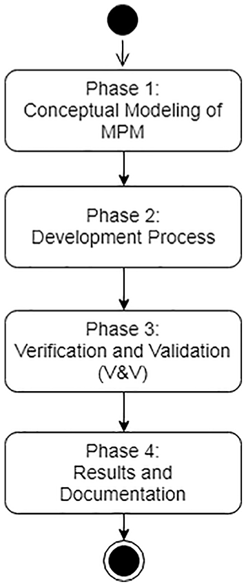
High-level view of MPMF.

Phase 2 is the development process of the actual MPM model construction. This phase includes the development activities of the MPM study: the implementation of the results and model(s) suggested by the Phase 1’s algorithm; the programming of the model(s); and the execution and calibration of the computer-generated (CG) model(s).

Phase 3 consists of the verification and validation (V&V) process. This phase takes place after the execution of the simulation and before the documentation of results to ensure credibility of the simulation study and the produced results. The relationship between Phase 2 and Phase 3 is iterative and frequent updates to the model may occur.

Finally, Phase 4 includes the preparation of the simulation report, the documentation of the results, and examination of future improvements.

3. Phase 1: Conceptual modeling of the MPM model

This section describes the conceptual modeling steps of the MPMF, which is composed of the activities illustrated in Figure 2. The framework integrates steps from a typical M&S methodology for implementing a single-method model^{1, 51} with steps from a methodology for combining DE and SD models.^{28, 44} The novel components in the framework include: steps for the integration of AB models; an algorithm that helps the user select appropriate M&S methods; steps for the identification of interaction points; and types of interaction for all three methods.

Figure 2.

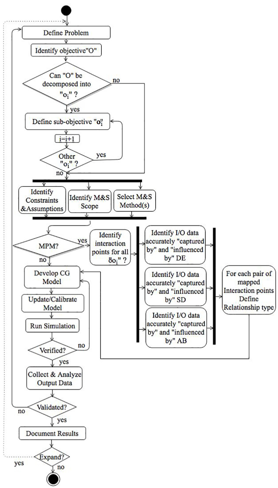
Activity diagram of internal view of MPMF.

3.1. Define problem

The first step the user needs to perform is to explicitly define the main problem and its surrounding environment. The challenge to define a problem well and agree upon specifications due to diverse opinions of the team⁵² has been tackled in soft-systems methodology as proposed by Checkland.⁵³ Appropriate time and effort must be invested on understanding and clearly defining the problem before starting to seek solutions.

3.2. Identify objective(s) “O” and decompose them into sub-objectives “o_i”

The next step is to identify the objectives of the M&S study by following the third principle of modeling, known as “divide and conquer”⁵⁴ or as “decomposition of the main purpose.”⁵⁵ According to the third modeling principle,⁵⁴ the user has to decompose the overall objective “O” of the study into sub-objectives “o_i.”

The decomposition of the overall objective into smaller objectives assists in considering each of the stakeholders’ problem formulations and in selecting the appropriate M&S method within a real-world systems context that may require a MPM approach to analysis.

If the overall objective “O” cannot be decomposed to smaller sub-objectives “o_i,” the user follows three parallel activities (Figure 3): “Identify Assumptions and Constraints,”“Identify M&S Scope,” and “Select M&S Method(s).” Otherwise, the user decomposes “O” into “o_i” and conducts the three parallel activities for each “o_i.” The objectives and sub-objective are defined prior to the selection of M&S method, or prior to possible revisions of current deployed simulations.^{56, 57} Moreover, the identification of constraints and assumptions, M&S scope and M&S method should be conducted concurrently.

Figure 3.

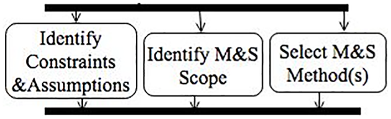
High-level view of Phase 1 of MPMF.

3.2.1. Identify constraints and assumptions

Following the decomposition of the main objective into sub-objectives, the user is directed to the identification of the assumptions and constraints under which the MPM study is performed. The defined assumptions and constraints play an essential role for the successful V&V of the simulation model.

Constraints may include environmental conditions that can restrict the possibilities of particular actions’ occurrence, or specific attributes that may need to be satisfied for the execution of specific actions.⁵¹ If some of the objectives cannot be adequately achieved and/or constraints are violated while developing the scope, then the expectations of the study can be reduced and/or constraints may need to be turned off. Therefore, we strongly recommend that the user considers frequent feedback from the problem owners in regard to the modeling assumptions and rational of the model, timeline of the MPM study, access to applicable data, cost constraints, and other constrains associated with activities that depend on time, available resources, and/or conditions.

3.2.2. Identify M&S scope

The identification of the M&S scope helps to achieve the objectives without violating the given constrains and assumptions. Therefore, the user/modeler needs to clearly define the aspects that will be included in the M&S study for each sub-objective. The M&S scope is also very significant as it builds a strong bridge of communication between the problem owner and the modeler and it provides all the necessary information, clarifications, and expectations of both parties. Figure 4 presents the activity “Identify Scope,” which is composed of five parallel activities that the modeler has to define for each of the DE, SD, and AB model(s).

Figure 4.

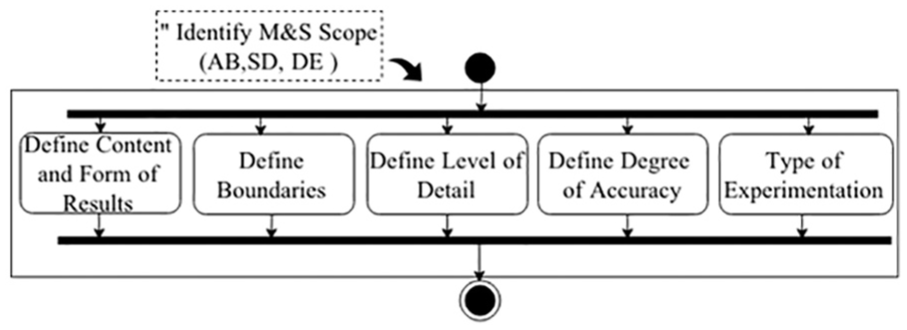
“Identify Scope” activity.

The sub-activities of “Identify Scope” are the following:

Define content and form of results: Content and form of results may vary from low (basic statistics) to high detail. For example, if an inclusive animation or very detailed statistics are expected for the simulation study, the time and effort engaged to implement a project may be considerably affected.⁵¹

Define boundaries: Four boundaries need to be defined: beginning, ending, upper, and lower boundaries (Figure 5). The beginning boundary is associated with the inputs that activate the model to start. The ending boundary is associated with the outputs of the simulated model. The upper boundary specifies the inputs that enter the model during the simulation execution time. The lower boundary specifies the outputs that exit the model during the simulation execution time.

Figure 5.

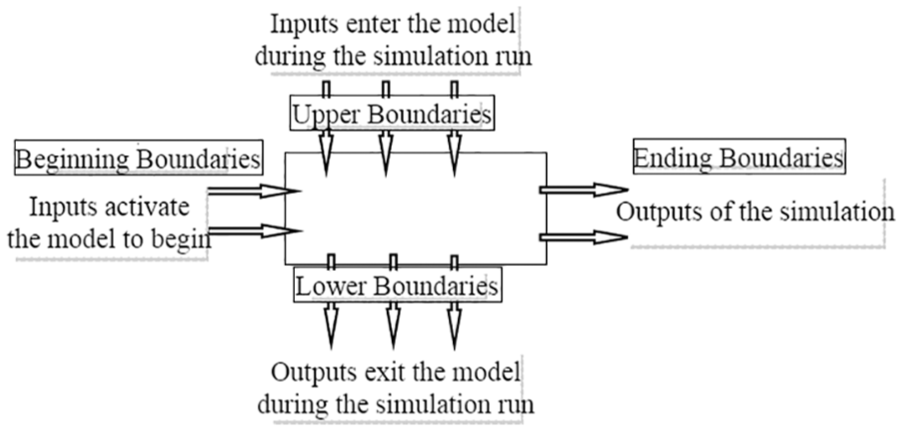
The four boundaries (beginning, ending, upper, and lower).

Define level of detail: The level of detail is defined by the level of required output precision and it is associated with factors such as: “detail” and “dynamic complexity”; size of the model; and time to develop and validate the model.⁵¹ Detail complexity is the type of high combinatorial complexity among various variables and attributes, while dynamic complexity is related with the interaction variables of the agents and their environment over time.^{3, 58} Figure 6 illustrates how the level of detail impacts a model’s development time. The more details a modeler adds in a model, the more the development time increases.

Figure 6.

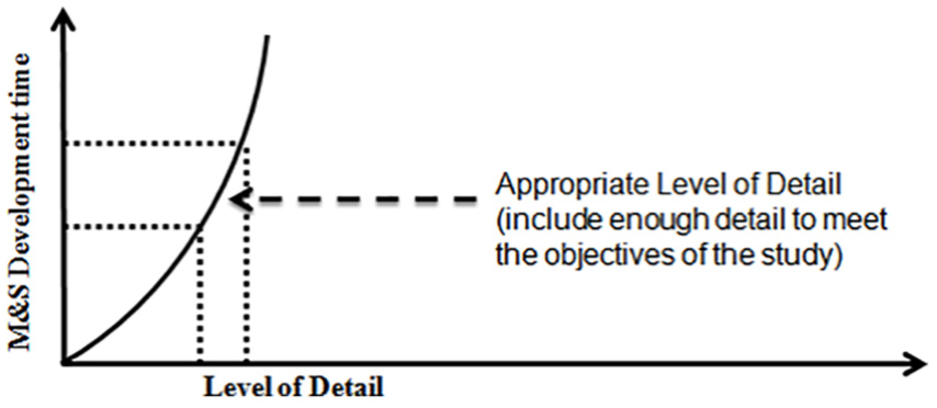
Impact of level of detail in terms of development time.

Define degree of accuracy: The degree of accuracy corresponds to the validity of data being employed. At this point, the user collects, prepares, and validates the input data before he/she starts the model development. The type of the collected data may be numeric or logic.⁵¹Numeric data define quantitative information according to the elements being modeled, such as costs, batch sizes, inter-arrival times, waiting times, and service times. Logic data describe the workflow of a model and capture information, such as model objects and their behaviors, policy rules, prioritization of processes, and assignment of resources.

Define type of experimentation: The type of experimentation specifies the type of analysis that will be conducted.⁵¹ For example, the user may conduct the analysis of capacity, sensitivity, decision response, comparison, optimization, and visualization.

3.3. Selection of M&S method(s)

In this activity, the modeler is prompted to select the M&S method(s) that best satisfy the decomposed sub-objectives o_i based on the problem, system, and methodology perspectives. The problem perspective refers to the understanding of the “nature, scope, and different aspects of the problem.”⁴⁴ The system perspective refers to “real world context under investigation.”⁴⁴ The methodology perspective refers to “philosophical assumptions, technical capabilities, limitations and inherent characteristics of the modelling method.”⁴⁴

Definition 1 : A criterion c_i∈ℂ is a reference point for the selection among the three M&S methods. Each criterion may be satisfied by up to three relevant variables of interest (VoI_ij). Each criterion is defined as in Equation (1):

c_{i} \in C where c_{i} {\begin{matrix} 1, if selected \\ 0, otherwise \end{matrix}

(1)

Definition 2 : A variable of interest (VoI_ij) represents the value associated with a criterion c_i and a j M&S method. Each VoI is defined as in Equation (2):

\forall o_{i} \in O, Vo I_{ij} = c_{i}, where j M & S method (DE, SD, AB)

(2)

Definition 3 : A weight w_ij is a numerical value assigned to a VoI_ij for a selected criterion c_i and a j M&S method. The value of a weight can range from 0 to 10: w_ij = 0, …, 10. Users can assign weights to each variable of interest based on the importance of the associated criterion, with 0 denoting the lowest importance and 10 the highest importance. The level of importance can be determined after communication with the stakeholders.

At this point, the framework aims to guide the user to select among the j most appropriate M&S method(s) based on the provided user input, where j = 1, 2, 3. An algorithm is applied to help the modeler select M&S method(s) for the model implementation as follows:

The modeler selects k number of criteria c_i∈ℂ (see Definition 1) that best fit the problem, system, and methodology perspectives of a particular objective o_i.

The modeler is called to assign numerical weights w_ij for each VoI_ij of k selected criteria c_i (see Definitions 2 and 3). This needs to be done in order to quantify the relative importance of each VoI_ij and provide a rational basis for the decisions being made.

All methods for each sub-objective are ranked from the best one to the worst one based on Equation (3), with best being the higher-scored method and worst the lower-scored method:

scor e_{method} = \max \sum_{j = 1}^{3} \sum_{i = 1}^{k} ({w_{ij}}^{*} Vo I_{ij})

(3)

The framework returns the higher-scored method for each sub-objective o_i.

The above steps of how the user/modeler interacts with the MPMF for the selected criteria c_i of an individual objective o_i are described by the UML sequence diagram of Figure 7. Table 1 provides a partial list of three alternative criteria considering the problem, system, and methodology perspectives for selecting among DE, SD, and AB M&S.

Figure 7.

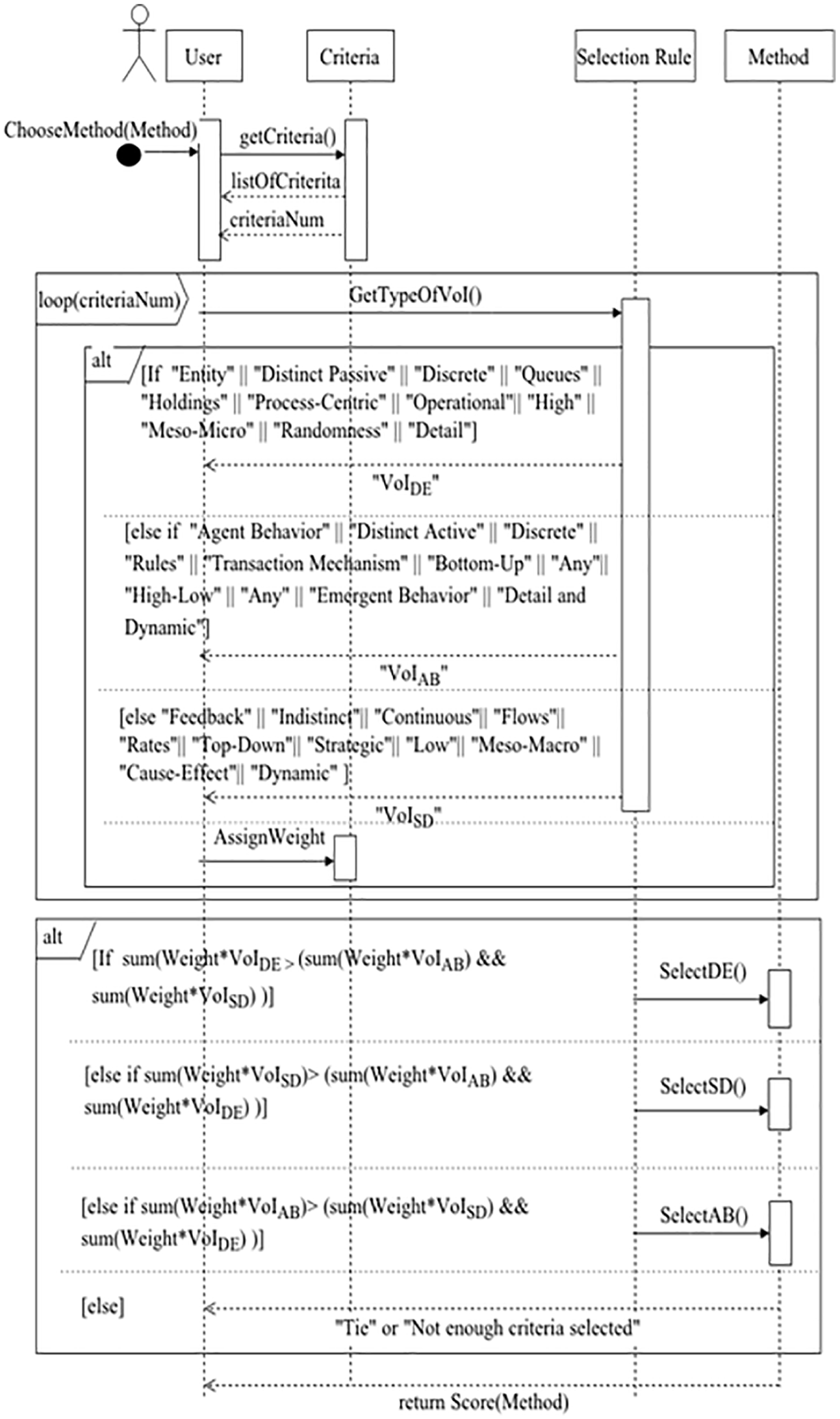
Selection of M&S method.

Table 1.

Sample list of MPMF criteria based on problem, system, and methodology perspectives.

Problem perspective
Criteria	Discrete Event	System Dynamics	Agent Based
Scope level	Operational tactical	Strategic	Any level
Situation	Queues	Flows	Rules
Required resolution	Detailed level	Aggregated level	More detailed level
System perspective
Criteria	Discrete Event	System Dynamics	Agent Based
Abstraction level	Meso–micro level	Meso–macro level	Any abstraction level
System process	Discrete	Continuous	System process
Control	Holding (queues)	Stock – rates	Control
Methodology perspective
Criteria	Discrete Event	System Dynamics	Agent Based
Modeling approach	Process centric	Top-down	Bottom-up
Object	Entity	Feedback	Agent
Time	Discrete	Continuous	Discrete

Once the M&S methods are selected for each sub-objective, the framework continues as follows:

If all “o_i” are described by a single M&S method, the conceptual modeling ends and the framework continues with Phases 2, 3, and 4.

If the sub-objectives are satisfied by different M&S methods, then the framework continues with the rest of the MPMF activities that are included in Phase 1 (sections 3.3 and 3.4) and the user is called to identify the interaction points for all “o_i.”

In the latter case, investigation of Q1 (“When and why is MPM required?”) takes place, while Q2 (“What are the interaction points?”) and Q3 (“How do AB, DE, and SD interact with each other over time to exchange information?”) will be investigated following the activities of sections 3.3 and 3.4.

In contrast to Chahal’s hybrid framework,⁴⁴ which suggests starting the development of the models before the identification of the interaction points and the mapping of their relationships, the MPM framework first conceptualizes the identification of interaction points and the type of information exchange between inputs/outputs (I/O) of the proposed models and then continues with the development of the actual models. The reason for altering this order is that we found it more practical to justify and conceptualize first how the modeling approaches can be connected and then implement the hybrid simulation. Furthermore, Chahal’s framework⁴⁴ focuses on the integration of DE and SD methods only in the healthcare domain, while the MPMF considers the integration of DE, SD, and AB modeling approaches for the development of simulation models in various domains.

3.4. Identify interaction points

The interaction points are defined as the pairs of I/O information exchange of data between different models.⁴⁴ The interaction points result from mapping the boundaries of the models that need to communicate. The mapping among DE, SD, and AB takes place prior to the development of a MPM model (answering Q2). The user/modeler is called to identify the interaction points, which consist of I/O data of DE, SD, and AB models and their corresponding variables that are properly “captured by” or “influenced by” each M&S approach, as illustrated in Figure 8.

Figure 8.

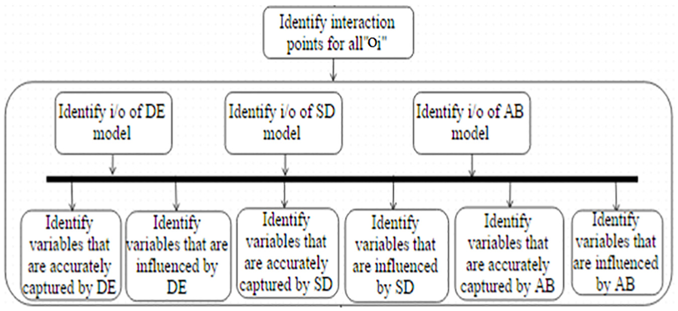
Variables “captured by” or “influenced by” DE, SD, and AB approaches.

3.5. For each pair of mapped interaction points define relationship type

This activity describes the type of interaction for each pair of mapped interaction points (answering Q3) that the user needs to define. In order to identify how AB, DE, and SD models interact with each other to exchange information, all the relationships among pairs of interaction points need to be well-defined. Table 2 describes the different types of interaction relationships that can be formed among DE, SD, and AB models. Chahal defined and proposed three generic types of relationships that can be formed between DE and SD interaction points: “direct replacement of variables,”“aggregation/disaggregation,” and “causal” relationships.⁴⁴ The present work further expands the generic relationships between the interaction points of information exchange to include AB as the number of relationships increases when AB is included. AB refers to a set of interaction rules for entities that produce complex behavior.

Table 2.

Types of relationship for interaction points.

Category	Types of relationship	Expressions	Examples
A. Value Assignment	A.1 Direct replacement	Value of AB variable = Value of SD or DE variable and vice versa of, or all possible combinations	The value of SD variable “number_of_not_treated_patients_per_day” = the value of DE variable “number_of_not_treated_patients” (Figure 10)
	A.2 Aggregation/ disaggregation	VarAB = Aggregated (equivalent variables or vectors in SD or DE) VarAB = Diseggregated (equivalent variables or vectors in SD or DE) The same expressions apply for all pair combinations	The SD rate of “arrivals_per_day” is disaggregated and passed to the DE entry point variable in the form of inter-arrival time (Figure 11)
	A.3 Causal relationships	VarAB = Math_Function (VarDE or SD) The same expressions apply for all pair combinations	“LossDueToLongWaitingTime” = “number_of_not_treated_patents_per_day”*“lost_profit_per_patient_not_treated” (Figure 14)
B. Impact statements	B.1 Add/remove/inject agents or entities	objectDE.inject(objectAB); objectAB.remove_objects(objectDE/SD); objectAB.add_objects(objectDE/SD); The same expressions apply for all pair combinations	The DE model adds entities to the AB population (patients) (Figure 12) The AB model removes entities from the DE process (Figure 13)
	B.2 Control flow	If, for, and while statements	The interaction between AB and DE is controlled by an if statement(Figure 13)
	B.3 Trigger event	The trigger type of the event can be: message, timeout, condition, rate, and arrival	Recurring event of timeout trigger type called “Update_not_treated_number “(Figure 10)
	B.4 State-chart control (combined with any of the previous types of relationship)	VarDE or SD = function (statechart.isStateActive(stateAB))	the AB state-chart state “LeaveClinic” is activated and executes a function (Figure 14)

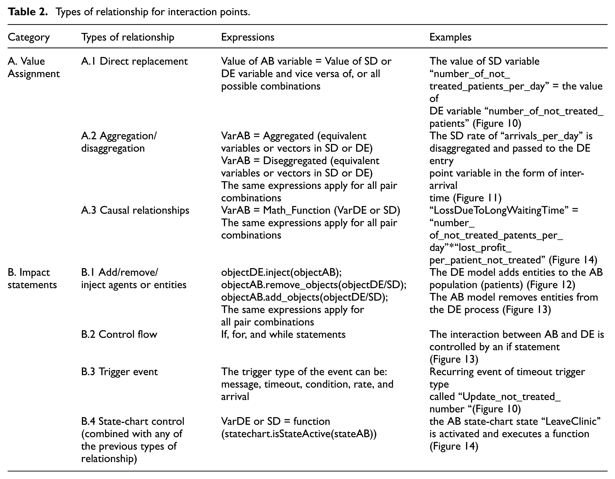
More specifically, AB interactions can involve state changes, inject, adding or removing objects or entities, transfer entities, control flow statements, trigger events, and state-chart control relationships. Therefore, we define two main categories and their subcategories to describe relationships of interaction points that involve information exchange among DE, SD, and AB. These two categories are the “value assignment” relationships (type A) and the “impact statements” relationships (type B).

As value assignment relationships, we define the relationships that include mathematical formulations and replacement of values between equivalent variables. This category consists of the three subcategories that were adapted by Chahal.⁴⁴

The “direct replacement of values of variables” (type A.1) corresponds to interaction points that represent equivalent variables of information exchange in both models.

The “aggregation/disaggregation” (type A.2) corresponds to interaction points that seize values of information exchange that need to be aggregated (accumulated) or disaggregated from the one model to equivalent values of the other model.

“Causal relationships” (type A.3) correspond to interaction points that are described by explicitly mathematical relationships.

As impact statement relationships, we define relationships that cannot be expressed using value assignment relationships, but they are related to more abstract concepts. Each of the impact statement relationships may contain one or more, or combination, of value assignment relationships. Such impact statement relationships can be:

“Add/Remove/Inject/Transfer agents or entities” (type B.1).

“Control flow relationships” (type B.2), which correspond to “if,”“for,” and “while” statements and define the flow of a particular logic.

“Trigger Event relationships” (type B.3), which can be of a different type, such as timeout, message, condition, rate, and arrival.

“State-chart control” (type B.4) corresponds to the state that may control the flow among two models, update variables from other models, or trigger any other type of relationship.

For better understanding of how these relationships work in practice, a healthcare multi-method M&S example was developed using AnyLogic⁵⁹ simulation software. In this example, the three M&S methods were combined for simulating patients who arrive in a clinic and wait to receive treatment. If the waiting time is greater than a specific threshold, then the patient leaves the clinic for another healthcare provider.

In this case, DE captures the patient’s flow of the treatment process. When a patient arrives at the clinic, he/she waits in the queue for his/her turn to receive treatment or not and then exits the clinic. AB represents the decision-making logic of each patient when he/she waits for treatment or when he/she decides to leave the clinic. Finally, the SD model estimates cost and profitability loss for those patients that abandoned the clinic due to long waiting times. Figure 9 illustrates the deployment of all the three M&S methods together.

Figure 9.

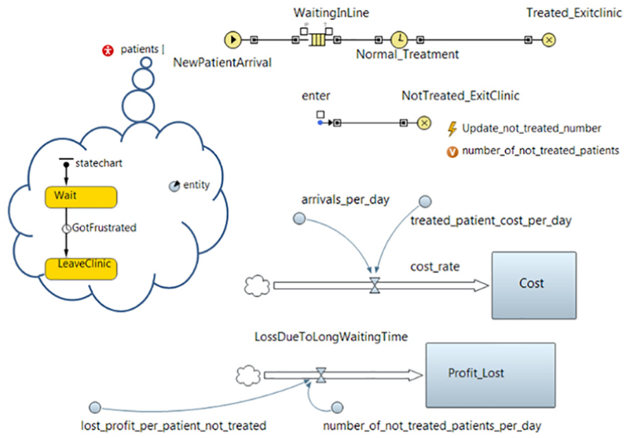
Deployment of DE, SD, and AB approaches.

During the simulation run time the DE model triggers the timeout event “Update_not_treated_number” (B.3 type), which, in turn, directly replaces the value of the SD variable “number_of_not_treated_patients_per_day” with its equivalent variable “number_of_not_treated_patients” that is calculated by the DE model (A.1 type). Figure 10 illustrates these types of relationships for the interaction between the DE and the SD models. In both models, the related interaction points represent variables whose values are equivalent to each other.

Figure 10.

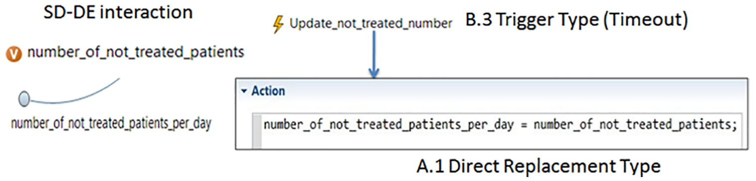
Combination of A.1 and B.3 type of relationships during SD–DE interaction.

Another type of relationship that takes place when SD and DE models interact is the disaggregation (A.2 type). More specifically, the SD rate of “arrivals_per_day” is disaggregated and passed to the DE entry point variable in the form of inter-arrival time (Figure 11). This type of relationship is type of disaggregation because the arrivals per day break down to smaller time intervals between each arrival.

Figure 11.

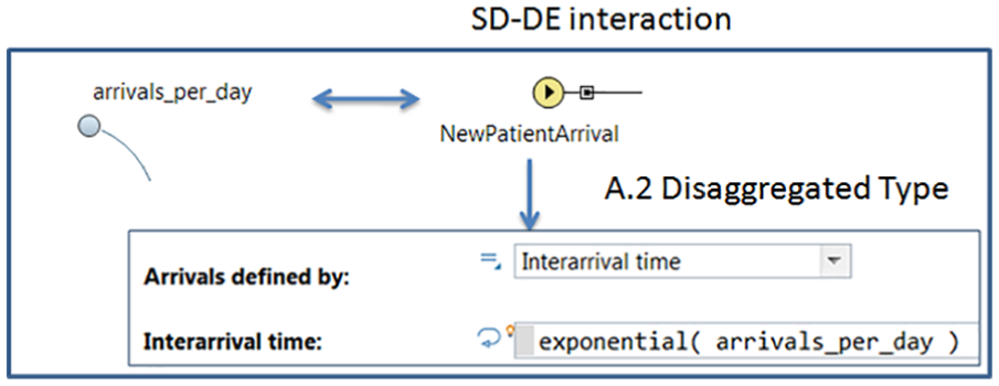
A.2 type of relationship during SD–DE interaction.

During the simulation interaction between the AB and DE models, the DE model adds entities to the AB population (patients). This “add entity” relationship type (B.1 type) is illustrated in Figure 12.

Figure 12.

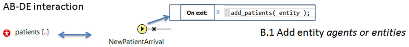
B.1 type of relationship during AB–DE interaction.

Figure 13 illustrates two types of relationship for interaction between AB and DE models. During the simulation run time, the AB Control flow (B.2 type) changes the process flow for the corresponding entity. More specifically, the AB transition removes (B.1 type) the corresponding entities, which can be either in the “WaitingInLine” or in the “Normal_Treatment” stage of the DE process. Then the AB transition transfers the corresponding entities into the “enter” object to exit the clinic.

Figure 13.

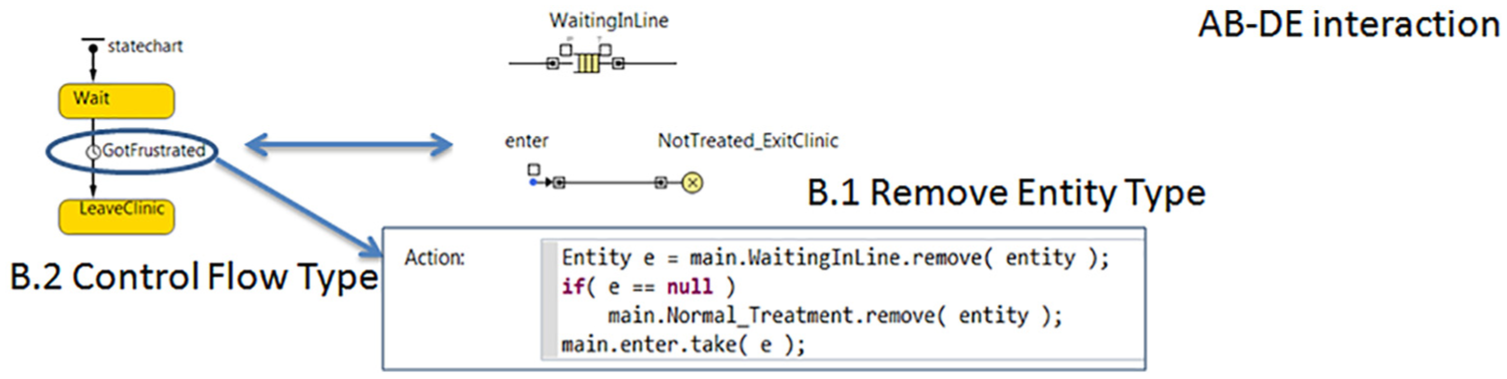
Combination of B.1 and B.2 type of relationships during AB–DE interaction.

Finally, during the interaction between AB and SD models, the SD variable “LossDueToLongWaitingTime” is controlled (B.4 type) by the AB state of “LeaveClinic.” When the AB state-chart state “LeaveClinic” is activated, the SD variable “LossDueToLongWaitingTime” is explicitly described by the mathematical expression (A.3 type) “number_of_not_treated_patents_per_day” multiplied by “lost_profit_per_patient_not_treated.”Figure 14 illustrates these two types of relationship.

Figure 14.

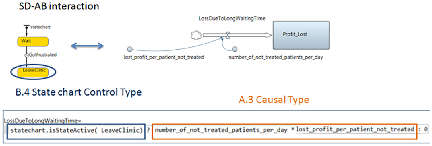
Combination of A.3 and B.4 type of relationship during SD–AB interaction.

Table 2 summarizes the two main relationship categories, the different types of relationships, and an expression example for each type.

Sections 4 to 7 present the steps that were followed when the MPMF was applied for the design, development, and evaluation of a universal task analysis simulation model (UTASiMo).

4. Following the MPMF methodology for the design, development, and evaluation of a universal task analysis simulation modeling tool – Phase 1: Conceptual modeling

Prior to the development of UTASiMo that deploys DE, AB, and SD models,⁶⁰ we followed the MPMF framework⁴⁹ as a guideline to justify the reasons for using each particular M&S method, as well as to conceptualize the identification of interaction points and the type of information exchange between inputs/outputs of the proposed models. Based on the user-defined objectives, assumptions, and selection of criteria, the framework suggested the development of a model consisting of three M&S methods. More specifically, we provide the methodology that was followed by applying the steps defined in section 3.

4.1. Define problem

Task analysis is a set of methods used in a work environment to evaluate human performance (i.e., task execution times, workload, human errors, etc.). The purpose of this study is to develop a simulation tool for task analysis that simulates human performance and predicts the level of human error and workload that human operators experience in order to meet the demanded task execution times. More specifically, the task analysis tool should be able to: (a) analyze task sequences and estimate task execution times; (b) take into account the human operator’s characteristics to estimate workload; and (c) consider task- and human operator-related properties to predict human error probabilities. Human error and workload depend upon the skills and experience of each human operator as well as the nature of the task (i.e., action or diagnosis tasks).

4.2. Identify overall objective “O” and decompose it into sub-objectives “o_i”

The overall objective is to develop a tool that predicts human error and workload that human operators experience in order to meet the demanded task execution times in a work environment. The overall objective of the model UTASiMo is to be capable of simulating tasks and scenarios performed by human operators, while considering task execution times and workload for operators with different skills/characteristics and assessing human error based on the skills of the operator and the dynamics of the task within a dynamic environment.

The overall objective is then decomposed to the following three sub-objectives:

o₁: Provide quantitative prediction of human error, which is influenced by the dynamics of the task and the properties of the operator over time.

o₂: Analyze a task network based on the task sequence, priorities, operator’s skills, and events to estimate task execution times.

o₃: Create a human operator model to capture variability in operator characteristics, indicate how the operators perform the tasks, and estimate utilization/workload.

4.2.1. Identify constraints and assumptions

As we mentioned earlier, assumptions are essential when creating a simulation model as it is not feasible to include all the possible events that will occur in reality. Therefore, during this system analysis, the following modeling constraints and assumptions are taken into consideration:

Each primary task can be performed by a single human operator.

Each human operator is assigned primary tasks in a sequence.

All task execution times are assumed to follow triangular distribution.

Human error is influenced by eight main factors.

The default walking speed for a human operator is 1.5 m/sec.

4.2.2. Identify M&S scope

The M&S scope is to develop a tool capable of automating the modeling process and simulating individuals performing tasks in various domains in order to estimate task execution times, utilization/workload and human error probabilities. The main purpose is to eliminate the need of programming and modeling efforts for generating task-based simulation models.

Define content and form of results

The content and form of results of this study require a high level of detail, including statistical I/O data analysis and visualization of the process through animation, graphs, and detailed statistics of the performance measurements such as average task execution time and average workload of human operators.

Define boundaries

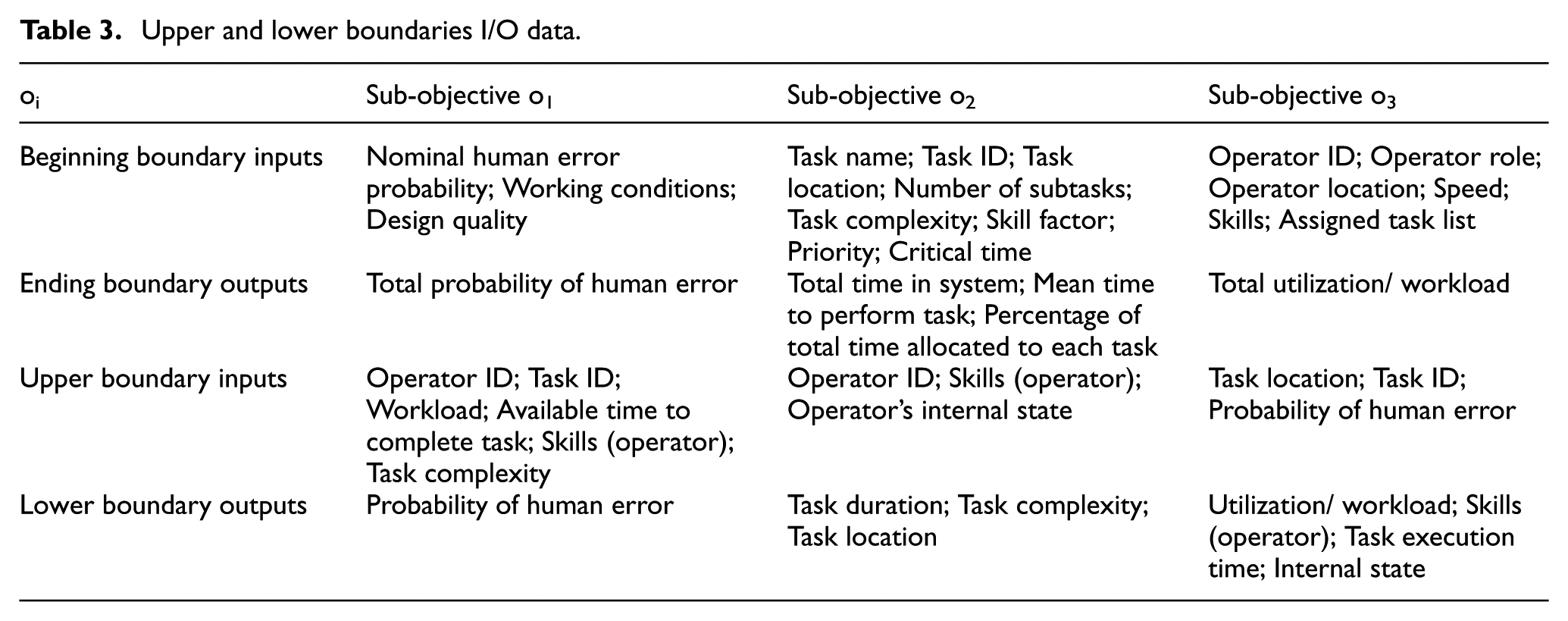
The next step is to define the boundaries and, more specifically, the beginning, ending, upper, and lower I/O data of information exchange, as well as the performance measurements that were considered for the V&V of the system. The beginning boundary data were used as input to calculate the performance measures (outputs). Table 3 illustrates the upper and lower I/O data information exchange among the three sub-objectives, the beginning boundary data, and the ending boundary data.

Table 3.

Upper and lower boundaries I/O data.

o_i	Sub-objective o₁	Sub-objective o₂	Sub-objective o₃
Beginning boundary inputs	Nominal human error probability; Working conditions; Design quality	Task name; Task ID; Task location; Number of subtasks; Task complexity; Skill factor; Priority; Critical time	Operator ID; Operator role; Operator location; Speed; Skills; Assigned task list
Ending boundary outputs	Total probability of human error	Total time in system; Mean time to perform task; Percentage of total time allocated to each task	Total utilization/ workload
Upper boundary inputs	Operator ID; Task ID; Workload; Available time to complete task; Skills (operator); Task complexity	Operator ID; Skills (operator); Operator’s internal state	Task location; Task ID; Probability of human error
Lower boundary outputs	Probability of human error	Task duration; Task complexity; Task location	Utilization/ workload; Skills (operator); Task execution time; Internal state

Level of detail, degree of accuracy, and type of experimentation

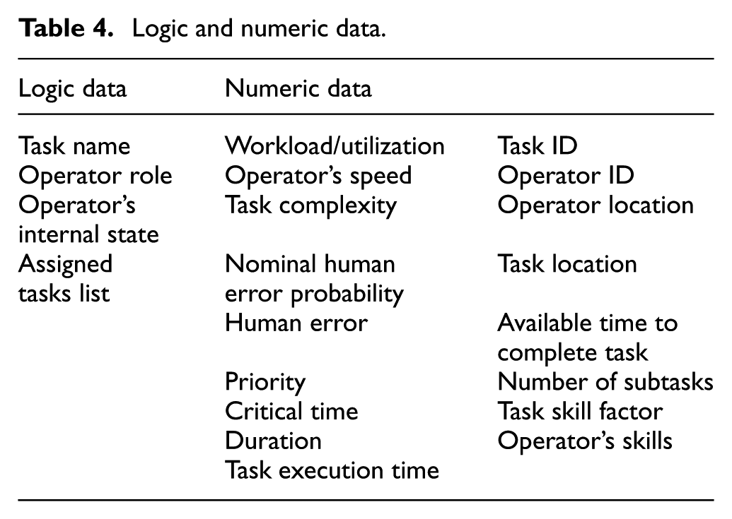
The experimentation type of this study includes the visualization of the system and validation of the UTASiMo-generated models. Table 4 illustrates the identification of logic and numeric data.

Table 4.

Logic and numeric data.

Logic data	Numeric data
Task name	Workload/utilization	Task ID
Operator role	Operator’s speed	Operator ID
Operator’s internal state	Task complexity	Operator location
Assigned tasks list	Nominal human error probability	Task location
	Human error	Available time to complete task
	Priority	Number of subtasks
	Critical time	Task skill factor
	Duration	Operator’s skills
	Task execution time

4.2.3. Selection of M&S method(s)

In this section, we run the MPMF framework by selecting criteria that fit the problem, system, and methodology perspective of each objective and assign their numerical weights based on their relevant importance, as described in section 3.3. Then, the additive functions are ranked from best to worst and the framework returns the higher-scored method for each sub-objective. Table 5 illustrates a partial list of selected criteria for each objective and assigned weights and summarizes the returned higher-scored M&S method for each of the three defined sub-objectives.

Table 5.

Selection of M&S methods.

Criterion	VoIs	Selection for sub-objective o₁	Weight w₁	Selection for sub-objective o₂	Weight w₂	Selection for sub-objective o₃	Weight w₃
Scope level	Operational	X			5
	Strategic		5			X
	Any			X			2
Situation	Queues	X			7
	Flows		7			X
	Rules			X			7
System process	Discrete	X			8
	Continuous		8			X
	Discrete/Continuous			X			5
Modeling approach	Process centric	X			7
	Top-down		5			X
	Bottom-up			X			5
Object	Entity	X			8
	Feedback		8			X
	Agent			X			10
Control	Holdings	X			10
	Stocks		10			X
	Transition mechanisms			X			10
Time	Discrete	X		X	8
Time	Continuous		8			X	8
M&S method selection		System Dynamics		Discrete Event		Agent Based

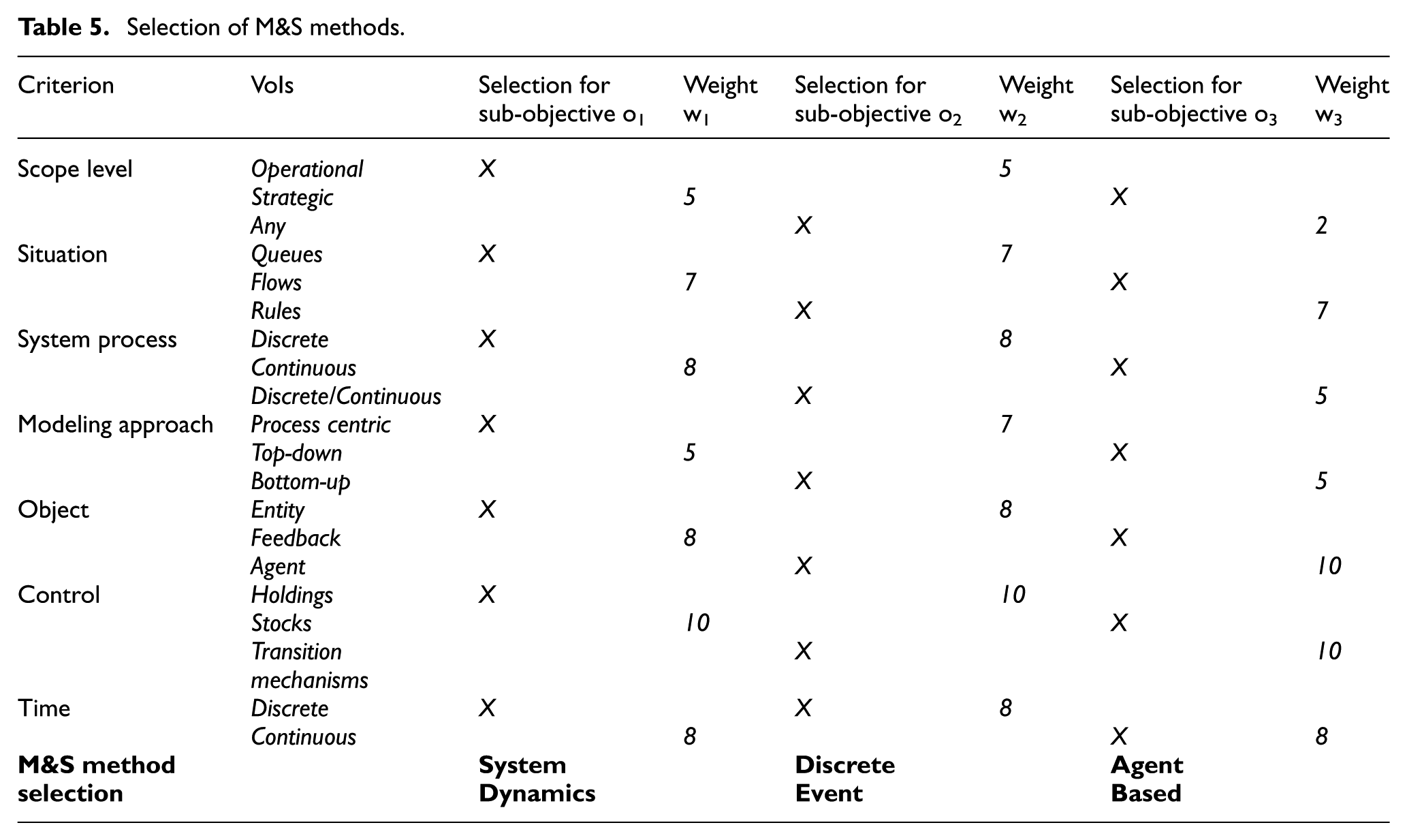
Here, it is important to capture the dynamic complexity between various variables affecting human performance (human error, workload, task execution times, skills, and experience) and analyze the way different variables influence human performance over time. For sub-objective o₁, the framework recommended SD as more appropriate to capture the dynamics of the environment that influence human error over time. The role of the SD model is to capture the causal relationships of factors affecting human error, use them to assess the overall simulated system’s human error probability, and provide a quantitative basis to the simulated system’s evaluation.⁶² For sub-objective o₂, the framework recommended DE to capture the temporal aspects of tasks, and for sub-objective o₃, the framework recommended AB to capture the human heterogeneity, behavior, and actions.⁶³

4.3. Identify interaction points

After selecting the M&S methods, the interaction points that describe variables of I/O information exchange among the different objectives need to be identified. In this case, we have three sub-objectives that are captured and influenced by three sub-models. These sub-models complement each other and form a MPM model capable of offering realistic perspective and useful insights. The mapping among DE, SD, and AB sub-models consists of input and output data of information exchange. Inputs and outputs of each model are paired with the inputs and outputs of the other models within the same perspective.

For the UTASiMo tool, the following types of interaction points and types of relationships are identified for each of the three interactions between pairs of objectives, based on section 3.5:

Interaction points between AB and DE models:

The operators (OperatorID (AB)) should be placed in a task network (OperatorID (DE)).

Each operator should be assigned a list of tasks (AssignedTaskList (AB)) in the task network (TaskID (DE)).

The operator should move to a specific task location in the task network to complete a task (Task Location (DE) – Task Location (AB)).

Each operator should complete a task based on a set of skills. Therefore, the task completion time in the DE model (Task Completion Time (DE)) will be affected by the skills of each operator in the AB model (Operator’s Skills (AB)).

The operator’s workload is defined as the percentage of time that the human operator is busy. Therefore, the workload of the operator in the AB model (Workload (AB)) will be affected by the duration of each task (Task Duration (DE)).

Interaction points between AB and SD models:

Humans may make mistakes that could lead to failure to perform a task correctly. Therefore, the human error model (Human Error (SD)) should be part of the operator (Agent (AB))

Operator’s workload (Workload (AB)) is one of the factors that may lead to human error and should be linked to the workload factor in the SD model (Workload (SD)).

Operator’s skills (Skills (AB)) is also one of the factors that affects human error and should be linked to the skill factor in the SD model (Skills (SD)).

Interaction points between DE and SD models:

Task complexity (Task_Complexity (DE)) is one of the factors that affects human error and should be linked to the task complexity factor in the SD model (Task_Complexity (SD)).

The available time left to complete a task (estimated duration of task (DE) – actual task completion time (DE)) also affects human error and should be linked to the available time factor in the SD model (Available_Time (SD)).

Table 6 summarizes the identified interaction types for each pair of interaction points. The types of relationship were identified based on section 3.5.

Table 6.

Type of interaction point and type of relationship.

	Interaction point	Type of relationship
Interaction points between AB and DE models	OperatorID (AB) – OperatorID (DE)	A.1 Direct replacement
	Task Completion Time (DE) – Operator’s Skills (AB)	A.3 Causal relationshipThe task completion time in the DE model is calculated based on a function that takes into account the skills of each operator in the AB model.
	Workload (AB) – Task Duration (DE)	A.3 Causal relationshipThe workload in the AB model is calculated based on a function that takes into account the estimated duration of each task in the DE model.
	AssignedTaskList (AB) – TaskID (DE)	A.2 Control flowWhile there are tasks in the operator’s list to be completed, the AB model transfers the execution of the task with specific TaskID to the DE model.
	Task Location (DE) – Task Location (AB)	A.1 Direct replacement
Interaction points between AB and SD models	Workload_(AB) – Workload (SD)	A.1 Direct replacement
	Skills (AB) – Skills (SD)	A.1 Direct replacement
	Human Error (SD) – Agent (AB)	B.4. State-chart controlThe AB state-chart transfers control to SD model to calculate error.
Interaction points between SD and DE models	Task Complexity_(DE) – Task Complexity_(SD)	A.1 Direct replacement
Interaction points between SD and DE models	Task Completion Time (DE) and Estimated Duration (DE) – Available_Time (SD)	A.3 Causal relationshipThe available time in the SD model is calculated based on a function that takes into account the task completion time of each task and the estimated duration in the DE model. If Task Completion Time (DE) > Estimated Duration (DE), then the Available_Time factor in the SD model is 5 (High), which increases the probability of error.

5. Phase 2: M&S development process

After completing the conceptual modeling phase of the UTASiMo task analysis tool, we move to the development process of it. The MPM model was implemented using AnyLogic software and consisted of three sub-models that interact with each other: a DE (Figure 15), a SD (Figure 16), and an AB (Figure 17) sub-model.

Figure 15.

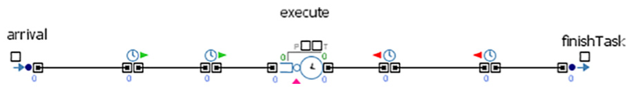
DE model of UTASiMo.

Figure 16.

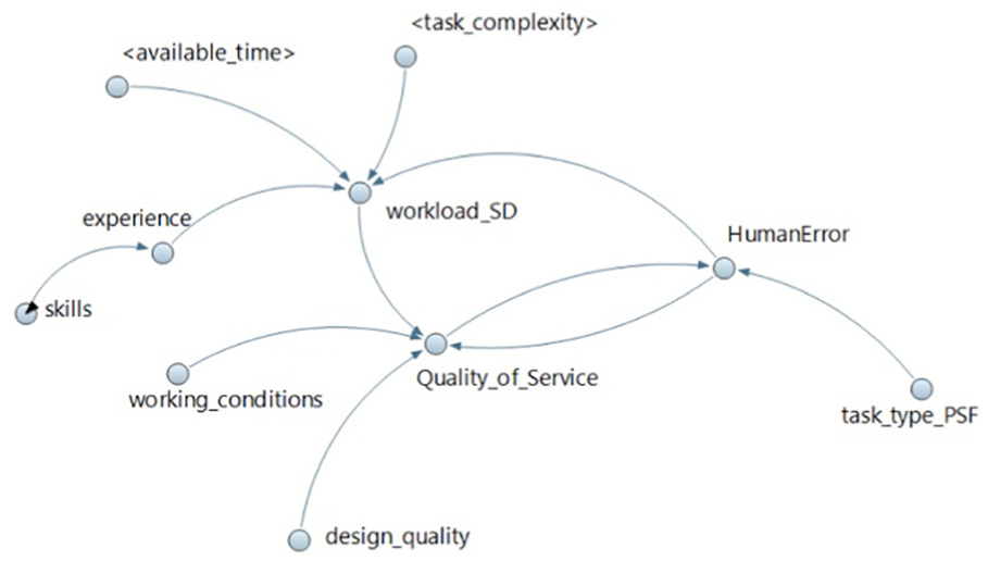
SD model of UTASiMo.

Figure 17.

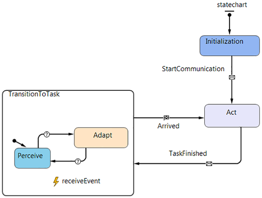
AB model of UTASiMo.⁶³

After selecting methods and identifying the interaction points, as described in sections 4.2.3 and 4.3, the DE simulation model was implemented as a network, where each node is a primitive task (discrete activity), such as a decision, perception, and/or physical activity. Nodes in the network have dependencies between them and form compound tasks. Task structure properties represented in the model are task ID, task name, number of subtasks, task location, task complexity, task skill factor, priority, duration, and critical time. The DE model is also responsible for collecting statistics in regard to the defined measurements of performance.

The human operators and their behaviors were implemented using hybrid SD–AB architecture. The hybrid architecture was suggested by the interaction point (Human Error (SD) – Agent (AB)) in section 4.3. Human operators were modeled as agents using a state-chart with three states (Figure 17)⁶³:

The state of Perception is an event-handler triggered by “receiveEvent” to check the environment for any event. Events can be either user-defined (i.e., alarm, stairs) or can be retrieved from the model (i.e., number of tasks to be executed, next task location, etc.).

The state of Adaptation includes a list of actions linked to their corresponding events. Each event may be linked to one or more actions. The agent selects the appropriate action based on the triggering event and the information gathered from the environment.

The state of Action includes the execution of a task or other event-triggered action.

The SD model that represents the human error contains eight main factors, four of which are interaction points and exchange data between the SD and the AB and DE models: workload, skills, available time, and task complexity. The SD model is depicted in Figure 16.

Overall, this multi-paradigm simulation model exchanges information through the paired DE–SD, AB–SD, and DE–AB interaction variables (Table 6). The detailed description of the M&S development process of the task analysis tool is not within the scope of this paper. More information about the development process can be found elsewhere.^{60, 62–65}

6. Phase 3: Verification and validation (V&V) of MPM model

Phase 3 provides information concerning the design as well as the V&V of the MPMF, using real-world data. More specifically, a MPM model of a power plant was produced using the UTASiMo tool to determine which system design produces the lowest average total time, workload, and human errors. The model was verified and validated using various techniques. First, the model was successfully tested for one human operator in order to verify the total task execution time. The model was verified and validated by observing the animation of the simulation output. Validation also included comparison of the simulated system behavior with the behavior of the real system. Figure 18 and Figure 19 show the animation of the model and the simulation results, accordingly. More information about the V&V process and documentation of results can be found elsewhere.^{60, 62–64}

Figure 18.

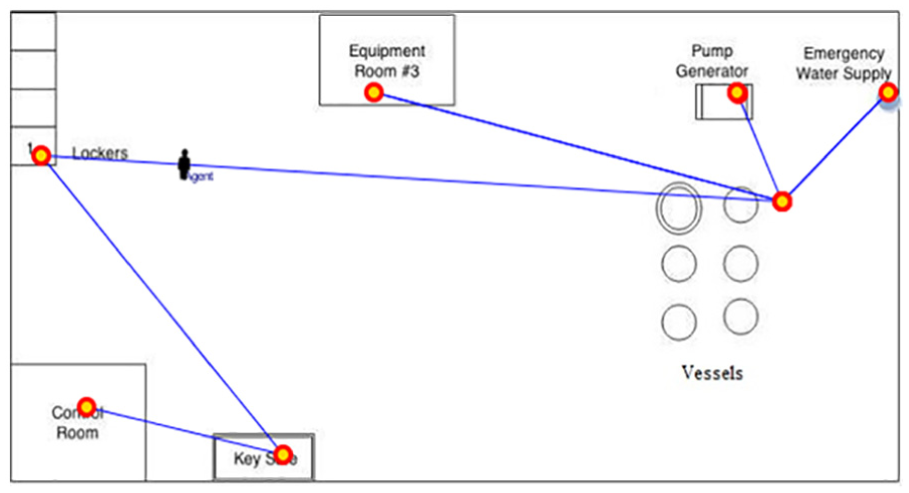
UTASiMo’s animation output.⁶³

Figure 19.

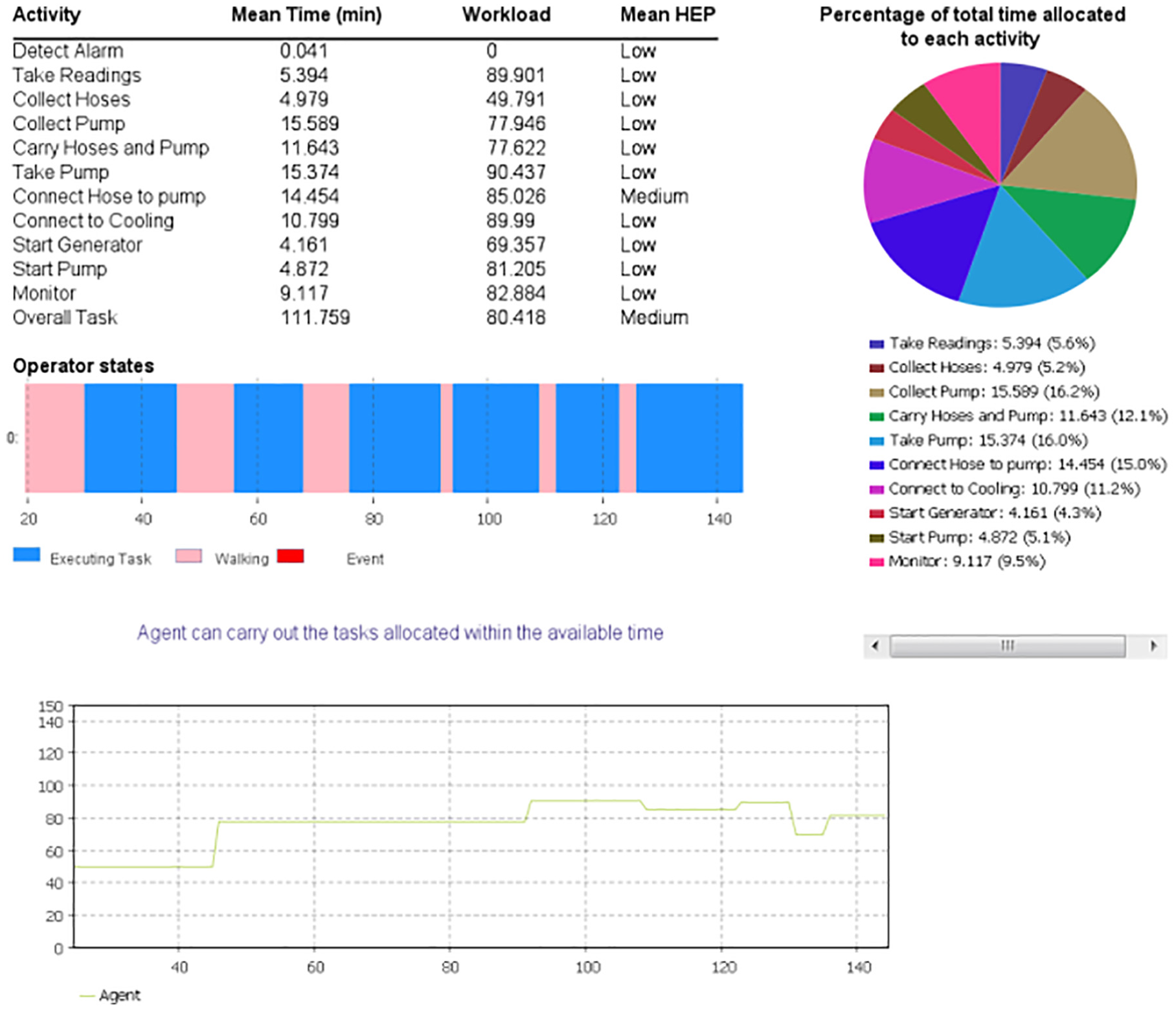
UTASiMo’s simulation results.

7. Phase 4: Discussion of results

The overall objective of this study was to provide a description of the MPMF framework and illustrate how it can be followed as a guideline to develop multi-paradigm simulation models utilizing different components. These components must be logically consistent, share common properties and behaviors, and be composable.⁹

In this case study, we showed how each component in the overall MPM model highlights a different aspect of the solution. The SD model helps to identify the factors that affect human error. These factors are then further evaluated in more detail using DE, which results in the identification of critical tasks (i.e., the tasks where an error is more likely to occur). Finally, the use of AB allows the modeling and evaluation of individual behavior on the task execution. However, the composability of the different components of the MPM model will be further investigated in future research.

Overall, the MPMF framework provided guidelines focused in the development of the conceptual modeling process. The framework was found helpful because it offers the option to combine and/or integrate three M&S methods, while other frameworks provide guidelines for one or combination of two M&S methods. The problem, system, and methodology perspective criteria of the framework aided the user to understand when and why each M&S method is more suitable. The criteria assisted the user to conceptualize and include aspects that would be impractical or even impossible to be captured by one or two M&S methods. Finally, the MPMF framework helped the user on how to connect the different models and formulate relationships between the interaction points.

8. Conclusions and future work

In this paper, a novel multi-paradigm modeling and simulation framework (MPMF) has been described. The MPMF provides guidance on how to design and develop a multi-paradigm model that addresses real-world systems’ problems. The use of the framework provides an effective approach for capturing the necessary information from a problem, system, and methodology perspective and for using it to integrate and/or combine different methods in such a way that benefits the design and implementation of the MPM simulation model.

The steps of the MPMF framework were explained and applied to a real case study for the development of UTASiMo. More specifically, the framework provided guidance on: (1) selecting the appropriate methods to be incorporated into the UTASiMo models; (2) defining what information will be exchanged among those models; and (3) deciding how the different models should be connected and interact with each other. This case study was presented to demonstrate the steps involved in the multi-paradigm model creation of a real-world system and to validate the MPM framework. The framework has also been successfully applied for the development of a multi-paradigm simulation model for an autonomous face recognition robotic system⁶⁶ as well as within the entertainment industry.

In general, the MPM models may be found useful when different M&S approaches need to be combined and/or integrated, as well as for future reusability. For example, one can enhance, reconfigure, and apply a pre-existing verified and valid module that has been used in a past MPM study to conduct another simulation study, since these models have been developed to communicate and interact with other models.

Our future work will also focus on applying the framework in different domains that require a MPM approach, as well as in the development of a decision support tool based on the MPMF framework.

Footnotes

Funding

This research received no specific grant from any funding agency in the public, commercial, or not-for-profit sectors.

Author biographies

Dr Konstantinos Mykoniatis holds a PhD and a MSc degree in modeling and simulation from University of Central Florida, and a BE degree in production engineering and management from Technical University of Crete. His research interests are in the areas of multi-paradigm modeling and simulation of complex and/or adaptive socio-technical systems and smart services, virtual and augmented reality, operations research, internet of things, and robotics technology.

Dr Anastasia Angelopoulou received her PhD in modeling and simulation from the University of Central Florida in 2015. She also holds a BSc degree in electronic and computer engineering from Technical University of Crete. Her research areas include modeling and simulation, simulation games, human factors, high performance computing, and simulation of p2p energy trading systems.

References

Law

McComas

. Simulation of manufacturing systems. In: Proceedings of the 30th conference on Winter simulation, Los Alamitos, CA, 13–16 December 1998. Washington, DC: IEEE Computer Society Press.

Bui

Lee

. An agent-based framework for building decision support systems. Decision Supp Syst 1999; 25(3): 225–237.

Sterman

. Business dynamics: Systems thinking and modeling for a complex world. Boston: Irwin/McGraw-Hill, 2000.

Brailsford

. Hybrid simulation in healthcare: New concepts and new tools. In: 2015 winter simulation conference (WSC), Huntington Beach, CA, 2015, pp. 1645–1653. Piscataway, NJ: IEEE.

Morel

Ramanujam

. Through the looking glass of complexity: The dynamics of organizations as adaptive and evolving systems. Organization Sci 1999; 10(3): 278–293.

Bonabeau

. Agent-based modeling: Methods and techniques for simulating human systems. Proc Natl Acad Sci USA 2002; 99(3): 7280–7287.

Borshchev

. The big book of simulation modeling. AnyLogic Company. XJ Technologies, 2013.

Powell

Mustafee

. Soft OR approaches in problem formulation stage of a hybrid M&S study. In: Proceedings of the 2014 winter simulation conference, Savannah, GA, 2014, pp. 1664–1675. Washington, DC: IEEE Press.

Mustafee

Brailsford

Djanatliev

Eldabi

Kunc

Tolk

. Purpose and benefits of hybrid simulation: Contributing to the convergence of its definition. In: 2017 winter simulation conference (WSC), Las Vegas. NV, 2017, pp. 1631–1645.

10.

Djanatliev

German

. Towards a guide to domain-specific hybrid simulation. In: IEEE proceedings of the 2015 winter simulation conference, Huntington Beach, CA, 2015, pp. 1609–1620. Washington, DC: IEEE Press.

11.

Borshchev

Karpov

Lebedev

. Distributed simulation of hybrid systems with HLA support. Parallel Comput Technol 2001; 2127: 410–420.

12.

Lynch

Padilla

Diallo

Sokolowski

Banks

. A multi-paradigm modeling framework for modeling and simulating problem situations. In: Tolk

Yilmaz

Diallo

Ryzhov

(eds) Proceedings of the 2014 winter simulation conference, Savannah, GA, 2014, pp. 1688–1699. Washington, DC: IEEE Press. Piscataway, NJ: IEEE.

13.

Tolk

Diallo

Padilla

Herencia-Zapana

. Reference modeling in support of M&S: Foundations and applications. J Simulation 2013; 7(2): 69–82.

14.

Shanthikumar

Sargent

. A unifying view of hybrid simulation/analytic models and modeling. Operations Res 1983; 31(6): 1030–1052.

15.

Vangheluwe

de Lara

Mosterman

. An introduction to multi-paradigm modelling and simulation. In: Barros

Giambiasi

(eds) The 2002 AI, simulation and planning in high autonomy systems conference. Lisbon, Portugal, April 2002, pp. 9–20.

16.

Nilsson

Peterson

Hudak

. Functional hybrid modeling. In: The PADL’03: 5th international workshop on practical aspects of declarative languages, 2003, pp. 376–390. Berlin and Heidelberg: Springer.

17.

Lei

Wang

Zhu

. A DSM-based multi-paradigm simulation modeling approach for complex systems. In: Pasupathy

Kim

S-H

Tolk

(eds) 2013 winter simulation conference, Washington, DC, 2013, pp. 1179–1190. Piscataway, NJ: IEEE.

18.

Fahrland

. Combined discrete event continuous systems simulation. Simulation 1970; 14(2): 61–72.

19.

Lättilä

Hilletofth

Lin

. Hybrid simulation models: When, why, how? Expert Syst Applic 2010; 37(12): 7969–7975.

20.

Tolk

Barros

D’Ambrogio

Rajhans

. Hybrid simulation for cyber physical systems: A panel on where are we going regarding complexity, intelligence, and adaptability of CPS using simulation. In: Proceedings of the symposium on modeling and simulation of complexity in intelligent, adaptive, and autonomous systems, Baltimore, ML, 2018, p. 3. San Diego, CA: Society for Computer Simulation International.

21.

Schieritz

Grobler

. Emergent structures in supply chains: A study integrating agent-based and system dynamics modeling system sciences. In: Dennis

(ed.) Proceedings of the 36th Annual Hawaii International Conference, Big Island, HI, 2003. Washington, DC: IEEE Press.

22.

Venkateswaran

Son

. Hybrid system dynamic–discrete event simulation-based architecture for hierarchical production planning. Int J Prod Res 2005; 43(20): 4397–4442.

23.

Helal

. Hybrid system dynamics-discrete event simulation approach to simulating the manufacturing enterprise. PhD Dissertation, University of Central Florida, 2008.

24.

Jovanoski

Minovski

Lichtenegger

Voessner

. Managing strategy and production through hybrid simulation. Indust Manag Data Syst 2013; 113(8): 1110–1132.

25.

Begun

Zimmerman

Dooley

. Health care organizations as complex adaptive systems. Adv Healthcare Org Theory 2003; 253: 288.

26.

Djanatliev

German

Kolominsky-Rabas

Hofmann

. Hybrid simulation with loosely coupled system dynamics and agent-based models for prospective health technology assessments. In: Laroque C, Himmelspach J and Pasupathy R (eds) Proceedings of 2012 IEEE winter simulation conference, Berlin, 2012, pp. 1–12. Washington, DC: IEEE Press.

27.

Djanatliev

Germ

. Prospective healthcare decision-making by combined System Dynamics, Discrete Event, and Agent Based simulation. In: Pasupathy

Kim

S-H

Tolk

(eds) Proceedings of 2013 IEEE winter simulation conference, 2013. Washington, DC: IEEE Press.

28.

Chahal

Eldabi

Young

. A conceptual framework for hybrid system dynamics and discrete event simulation for healthcare. J Enter Info Manag 2013; 26(1/2): 50–74.

29.

Djitog

Aliyu

Traoré

. A model-driven framework for multi-paradigm modeling and holistic simulation of healthcare systems. Simulation 2018; 94(3): 235–257.

30.

Martinez-Moyano

Macal

. A primer for hybrid modeling and simulation. In: Roeder

Frazier

Szechtman

Zhou

(eds) Proceedings of the 2016 winter simulation conference, Washington, DC, 2016, pp. 133–147. Washington, DC: IEEE Press.

31.

Scholl

. Agent-based and system dynamics modeling: A call for cross study and joint research. In: IEEE proceedings of the 34th annual Hawaii international conference on system sciences, Maui, HI, 2001, pp. 8. Washington, DC: IEEE Press.

32.

Phelan

. Using integrated top-down and bottom-up dynamic modeling for triangulation and interdisciplinary theory integration. In: Scholl

Phelan

(eds) The 22nd international conference of the System Dynamics Society, Oxford, 25–29 July 2004. Albany, NY: System Dynamics Society.

33.

Swinerd

McNaught

. Design classes for hybrid simulation involving agent-based and system dynamics models. Sim Model Pract Theory 2012; 25: 118–133.

34.

Mingers

Brocklesby

. Multimethodology: Towards a framework for mixing methodologies. Omega 1997; 25(5): 489–509.

35.

Dubiel

Tsimhoni

. Integrating agent based modeling into a discrete event simulation. In: Kuhl

Steiger

(eds) Proceedings of the winter simulation conference, Orlando, FL, 2005; pp. 1029–1037. Piscataway, NJ: IEEE.

36.

Petropoulakis

Giacomini

. A hybrid simulation system for manufacturing processes. Integr Manu Sys 1997; 8(4): 189–194.

37.

Rabelo

Helal

Jones

Min

. Enterprise simulation: A hybrid system approach. Int J Comp Integr Manu 2005; 18(6): 498–508.

38.

Zulkepli

Eldabi

Mustafee

. Hybrid simulation for modelling large systems: An example of integrated care model. In: Laroque

Himmelspach

Pasupathy

(eds) Proceedings of the winter simulation conference, Berlin, 2012, pp. 1–12. Piscataway, NJ: IEEE.

39.

Barros

. Towards a universal formalism for modeling & simulation. In: 2017 winter simulation conference (WSC), Las Vegas, NV, 2017, pp. 750–761. Piscataway, NJ: IEEE.

40.

Tolk

Page

Mittal

. Hybrid simulation for cyber physical systems: State of the art and a literature review. In: Proceedings of ANSS, Baltimore, ML, 2018, p. 10. Society for Computer Simulation International.

41.

Brailsford

Eldabi

Kunc

Mustafee

Osorio

. Hybrid simulation modelling in operational research: A state-of-the-art review. Euro J Op Res 2018. in press.

42.

Glazner

. Understanding enterprise behavior using hybrid simulation of enterprise architecture. PhD Thesis, Engineering Systems Division, Massachusetts Institute of Technology, Cambridge, MA, 2009.

43.

Ross

Ulieru

Gorod

. A multi-paradigm modeling and simulation approach for systems of systems engineering: A case study. In: Cook S, Ireland V, Gorod A, Ferris T and Do Q (eds) Proceeding of the IEEE 9 international conference on system of systems engineering. Stamford Grand, Glenelg, Adelade, SA, 2014, pp. 183–188. Washington, DC: IEEE.

44.

Chahal

. A generic framework for hybrid simulation in healthcare. PhD Dissertation, Brunel University School of Information Systems, UK, 2010.

45.

Balaban

. Toward a theory of multi-method modeling and simulation approach. PhD Dissertation, Old Dominion University, Norfolk, VA, 2015.

46.

Lorenz

Jost

. Towards an orientation framework in multi-paradigm modeling. In: Proceedings of the 24th international conference of the System Dynamics Society, Nijmegen, The Netherlands, 23–27 July 2006, pp. 1–18. Albany, NY: System Dynamics Society.

47.

Pidd

. Computer simulation in management science. 5th ed. John Wiley and Sons Ltd, 2004.

48.

Mykoniatis

Karwowski

. A Generic framework for multi-method modeling and simulation in complex systems. In: IEEE SSCI 2014 dissertation consortium, Orlando, Florida, 9–12 December 2014. Washington, DC: IEEE.

49.

Mykoniatis

. A generic framework for multi-method modeling and simulation of complex systems using Discrete Event, System Dynamics, and Agent Based approaches. PhD Dissertation, University of Central Florida Orlando, Florida, 2015.

50.

Balaban

Hester

Diallo

. Towards a theory of multi-method M&S approach: Part I. In: Tolk

Yilmaz

Diallo

Ryzhov

(eds) Winter simulation conference, Savannah, GA, 2014, pp. 1652–1663. Piscataway, NJ: IEEE.

51.

Harrington

Tumay

. Simulation modeling methods: To reduce risks and increase performance. New York: McGraw-Hill, 2000, pp. 1–3, 379.

52.

Vennix

. Group model-building: Tackling messy problems. Sys Dynamics Rev 1999; 15(4): 379–401.

53.

Checkland

. Soft systems methodology: A thirty-year retrospective. Sys Res Behavioral Sci 2000; 17: S11–S58.

54.

Pidd

. Tools for thinking. 2nd ed. John Wiley & Sons, 2003.

55.

Powell

. The teacher’s forum: Six key modelling heuristics. Interfaces 1995; 25(4): 114–125.

56.

Robinson

. Conceptual modeling for simulation: Issues and research requirements. In: Lawson

Liu

Perrone

Fred Wieland

(eds) Proceedings of the 38th conference on winter simulation, Monterey, CA, 2006, pp. 792–800. Piscataway, NJ: IEEE.

57.

Robinson

. Conceptual modelling for simulation. Part II: a framework for conceptual modelling. J Op Res Soc 2008; 59(3): 291–304.

58.

Sterman

. Learning in and about complex systems. Sys Dynam Rev 1994; 10(23): 291–330.

59.

XJ Technologies Company Ltd, AnyLogic, https://www.anylogic.com/ (n.d., accessed February 2019).

60.

Angelopoulou

. A simulation-based task analysis using agent-based, discrete event and system dynamics simulation. PhD Dissertation, University of Central Florida, Orlando, Florida, 2015.

61.

Akbas

Mykoniatis

Angelopoulou

Karwowski

. A model-based approach to modeling a hybrid simulation platform (work in progress). In: Proceedings of the symposium on theory of modeling and simulation-DEVS integrative. Tampa, FL, 13 April 2014, pp. 1–6. San Diego, CA: Society for Computer Simulation International.

62.

Angelopoulou

Mykoniatis

. The system dynamics architecture of UTASiMo: A simulation-based task analysis tool to predict human error probability. In: IEEE CogSima 2017, pp. 1–13. Savannah, GA, Washington, DC: IEEE.

63.

Angelopoulou

Mykoniatis

. UTASiMo: A simulation-based tool for task analysis. Simulation 2018; 94(1): 43–54.

64.

Angelopoulou

Mykoniatis

Karwowski

. A framework for simulation based task analysis. IEEE CogSima 2015, Orlando, Florida, 2015, pp. 77–81. Washington, DC: IEEE Press.

65.

Angelopoulou

Karwowski

. Universal task model for simulating human system integration processes. In: IEEE SSCI 2014 dissertation consortium, Orlando, Florida, 9–12 December 2014. Washington, DC: IEEE.

66.

Mykoniatis

Angelopoulou

Soyler-Akbas

Hancock

. Multi-method modeling and simulation of a face detection robotic system. In: 2016 annual IEEE systems conference (SysCon), 2016, pp. 1–6. Washington, DC: IEEE Press.

A modeling framework for the application of multi-paradigm simulation methods

Abstract

Keywords

1. Introduction

1.1. A brief review of hybrid simulation solutions

1.2. Current work

2. Overview of the multi-paradigm modeling framework (MPMF)

3. Phase 1: Conceptual modeling of the MPM model

3.1. Define problem

3.2. Identify objective(s) “O” and decompose them into sub-objectives “oi”

3.2.1. Identify constraints and assumptions

3.2.2. Identify M&S scope

3.3. Selection of M&S method(s)

3.4. Identify interaction points

3.5. For each pair of mapped interaction points define relationship type

4. Following the MPMF methodology for the design, development, and evaluation of a universal task analysis simulation modeling tool – Phase 1: Conceptual modeling

4.1. Define problem

4.2. Identify overall objective “O” and decompose it into sub-objectives “oi”

4.2.1. Identify constraints and assumptions

4.2.2. Identify M&S scope

4.2.3. Selection of M&S method(s)

4.3. Identify interaction points

5. Phase 2: M&S development process

6. Phase 3: Verification and validation (V&V) of MPM model

7. Phase 4: Discussion of results

8. Conclusions and future work

Footnotes

Funding

Author biographies

References

3.2. Identify objective(s) “O” and decompose them into sub-objectives “o_i”

4.2. Identify overall objective “O” and decompose it into sub-objectives “o_i”