
Abstract
Understanding the true nature of viscoelastic behaviors in multi-physical systems has always been a challenging issue in system dynamic investigations, as each existing physical subdomain of the system may follow a different attenuation pattern during the dynamic process. In this study, to generate a viscoelastic model suitable for multi-physical domain dynamic investigations, a physical combined viscoelastic model is proposed. To this aim, by means of the bond graph approach, an energy-based conventional viscoelastic model is first generated, and its embedded dispersive mechanisms are interpreted physically. By including the interpreted dissipative mechanisms into the relative subdomains of an elastic domain, an energy-based combined viscoelastic model is then proposed. The obtained simulation results indicate that the proposed viscoelastic model is able to capture a variety of viscoelastic behaviors in the system with respect to the true physical nature of the system.
Keywords
1. Introduction
To a high degree, elasticity is a suitable characteristic for modeling wave propagation through materials. No real materials, however, are perfectly elastic, but rather are anelastic. In a real medium, wave energy is gradually converted into heat. The attenuation of propagated waves in some cases, such as in viscoelastic materials, is quite significant and could be a source of erroneous results in forward modeling, inversion, and imaging if neglected. 1 Thus, analyzing the mechanics of viscoelastic materials has been proven to be extremely challenging.
Many classical viscoelastic models of materials have been put forward, such as the Maxwell, the Voigt, and the Standard Linear Solid (SLS) models.2,3 In addition, various fractional viscoelastic models of materials have been presented and their constitutive relations discussed.4–8 In these models, the existing viscoelastic dynamics are presented using mechanical analogous components (such as springs and dashpots) and curve fitting techniques. The resultant models merely mimic the observable behaviors of the systems, and do not include the compound physical connections between the parameters (e.g., material and geometrical parameters) of the systems. They do not, therefore, adequately expose the physical concepts of viscoelasticity underpinning the dynamics of the systems.
The problem associated with conventional modeling techniques can generally be traced back to the use of the dispersive mechanisms (e.g., retardation and relaxation mechanism)9–11 that only pay attention to the regeneration of the attenuated dynamics of the systems and ignore the true casual interactions between the energetic components (e.g., capacity, inertia, and resistivity) of the systems. This negligence leads to the separation of the models from their intended internal energetic behaviors of the systems, and results in a limited applicability of these models. Given that the viscoelastic behavior of a system is a true reflection of the kinetic, potential, and energetic interactions of the thermal subdomains of the system, the conventional models are deemed to be unsuitable for multi-physical system dynamic investigations.
The non-physical nature of the conventional models also limits the valid ranges of these models, as frequently reported in the literature. Being disconnected from the physics of the systems, the generated models rely on combined parameters (such as relaxation time) to produce the dispersive behaviors of the systems. This makes the models incapable of distinguishing the dynamics of the same shape but different nature, and they are thus unable to reveal specific physical behaviors of the systems on the level of their ongoing phenomena. Although attempts have been made to broaden the valid ranges of these models by employing more dispersive mechanisms that are activated in difference frequencies (e.g., the Maxwell–Wiechert model 12 ), the added combined parameters are still unable to include the missing physics in the models that allow the tracking of the physical phenomena within the systems.
Given the deficiencies associated with the conventional models, it becomes obvious that a physical viscoelastic model will be desirable if the ability to capture and track the continuing viscoelastic behavior of a system is of concern. The required model should employ typical parameters that can carry distinctive physical meanings of the system, and should provide ongoing dynamics that can reveal clear energetic interactions between involved physical components of the system. The level of physical detail contained in such a model will decide the range of suitabilities for the model’s application.
To generate such a physical viscoelastic model suitable for multi-physical system dynamic investigations, the bond graph (BG) modeling technique13–19 is suggested in this paper. Working on the basis of physical system theory, the BG technique provides a continuous power exchange frame between the existing physical subdomains of a multi-physical system, and produces the behavior of the system on the basis of power conservative interactions between the existing energetic components of the system. The model thus generated is analytical in nature while potentially reflecting the true physical meaning of the system. This physical model then provides a meaningful insight of the ongoing dynamics in viscoelastic phenomena.
The embedded physical lucidity of the proposed viscoelastic model can also provide a physical explanation to the limitations of the conventional models and, thus, lead to the development of a more physical approach that can extend the valid range of the generated model. In addition, using the BG approach, the domain-independency of the proposed approach can provide a low-cost dynamic coupling capability between the generated model and the models of other subdomains. This capability is particularly beneficial for multi-physical domain dispersive dynamic investigations. It also provides a desirable basis for the design of applicable control strategies to identify and suppress the undesired behavior of the system.
To develop the proposed viscoelastic model, the remainder of this paper is organized as follows. In Section 2, the fundamentals of viscoelasticity in the mechanical domain and the problem relating to the implementation of the conventional methods are explained. An energy-based conventional viscoelastic model is then generated in Section 3 using the BG terminology, and the physical interpretation of the viscoelastic phenomena occurring inside the model is explained. By employing the obtained physical dispersive mechanisms, an inclusive viscoelastic model incorporating all aspects of energy dissipation of the system is proposed. In Section 4, the simulation results of the proposed energy-based combined viscoelastic model together with its conventional counterparts in BG representations are analyzed, and their corresponding capabilities in capturing the viscoelastic behavior of the system are demonstrated. The entangled viscoelastic behavior of material is then concluded in Section 5, where the use of the proposed viscoelastic model is justified and the reason for the limited applicability of the conventional models is revealed.
2. Fundamental issues of conventional viscoelasticity
From the literature, the fundamentals of viscoelasticity are mainly interpreted on the basis of the observed behavior of a system, not on the basis of the energetic interaction within a system. The theory of viscoelasticity 10 and its associated issues can be highlighted as follows.
The basic hypothesis in conventional viscoelastic theory focuses on the fact that the current value of the stress tensor depends on the history of the strain tensor.11,20 Considering the linear functional and continuous strain history, the Riesz representation theorem 21 allows the function to be rewritten as a convolution integral:
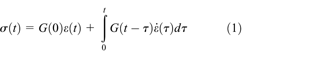
where
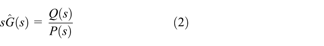
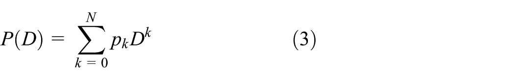
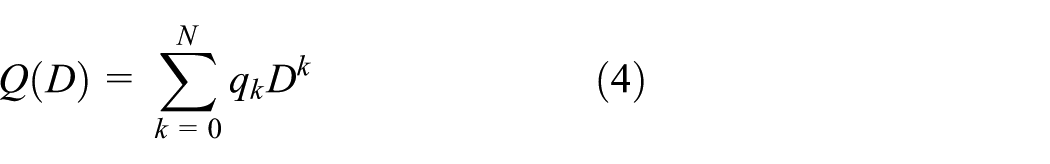
where pk and qk are polynomials,

By taking the Laplace transform of Equation (5), one has the following:
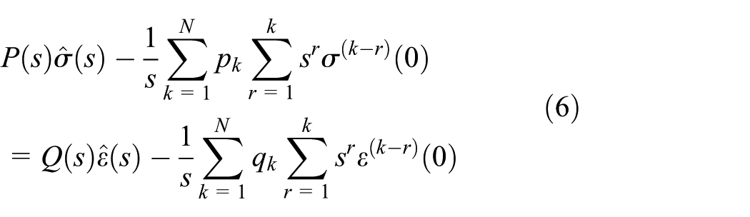
Assuming that the order of
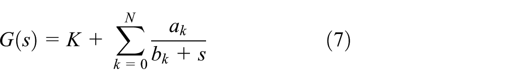
By taking the inverse Laplace transform of Equation (7), the general solution for
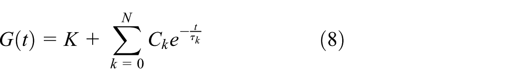
The obtained
It is clear that in the theory of viscoelasticity the attempt is to generate a fading functional between the stress and strain of the system, whereas the actual viscoelastic behavior of the system is a result of the interactive dynamics of the system energetic components. Since these internal interactions are not observable, they are not tractable in an experimental attempt. Accordingly, the majority of the conventional viscoelastic models using this theory such as the Maxwell, the Voigt, and the SLS models, 22 can only show the relaxing behavior of the system without paying attention to the physical reasons behind the phenomena. Although a conventional model can be a useful tool for investigating the relaxing behavior of the system, the literature shows the low capability of such a model in covering the whole range of relaxation dynamics of a system, 22 especially in the case of a multi-physical system where the role of the internal interactions becomes more significant.
In a conventional viscoelastic model, although the molecular motion of the system can be visualized by allocating the analogous mechanical elements, spring and dashpot,
5
in the form of the Maxwell and Voigt arms shown in Figure 1, the introduced combined parameters of the model (such as the relaxation time
where for the analogous mechanical component of the model,
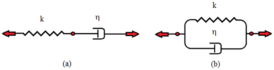
Viscoelastic model: Maxwell arm (a); Voigt arm (b).
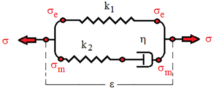
Standard Linear Solid viscoelastic model.
3. Energy-based viscoelastic model: a physical approach
To find the relation between a viscoelastic model and the energetic behavior of its corresponding system, the energetic interaction of the dispersive mechanism is required to be defined with respect to the involving subdomains of the system. To achieve this, in this paper it is proposed that a dispersive model for each involving subdomain is first generated, and the generated models are then combined in a power continuous form. By doing so, it is anticipated that the resultant model of the system will automatically capture the various physical phenomena occurring inside the system, including the viscoelastic phenomena.
To generate a physical dispersive model for each of involving subdomains, one needs to identify the dissipation nature of different subdomains. To do this, a physical explanation of the existing entropic behavior of the conventional viscoelastic models is identified by means of the BG approach. The comparison between the physical interpretation of the existing dispersive mechanisms (relaxation and/or retardation) of the conventional viscoelastic models and that of the energy dissipative components of each subdomain can lead to the identification of the assortment of the dispersive mechanisms that can form an energy-based viscoelastic model.
In the following, the procedure explained above will be conducted to generate the proposed energy-based viscoelastic model for a one-dimensional (1D) reticulated structure.
3.1. Domain-independent pure elastic models
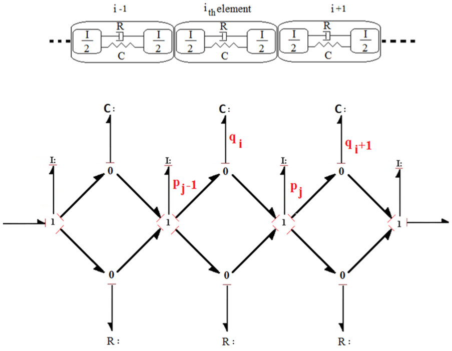
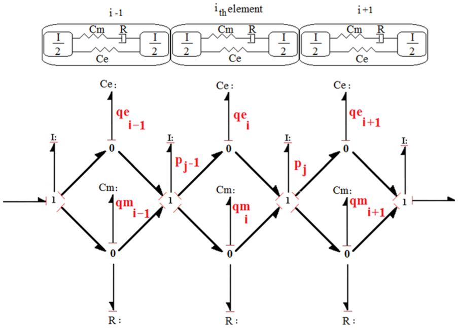
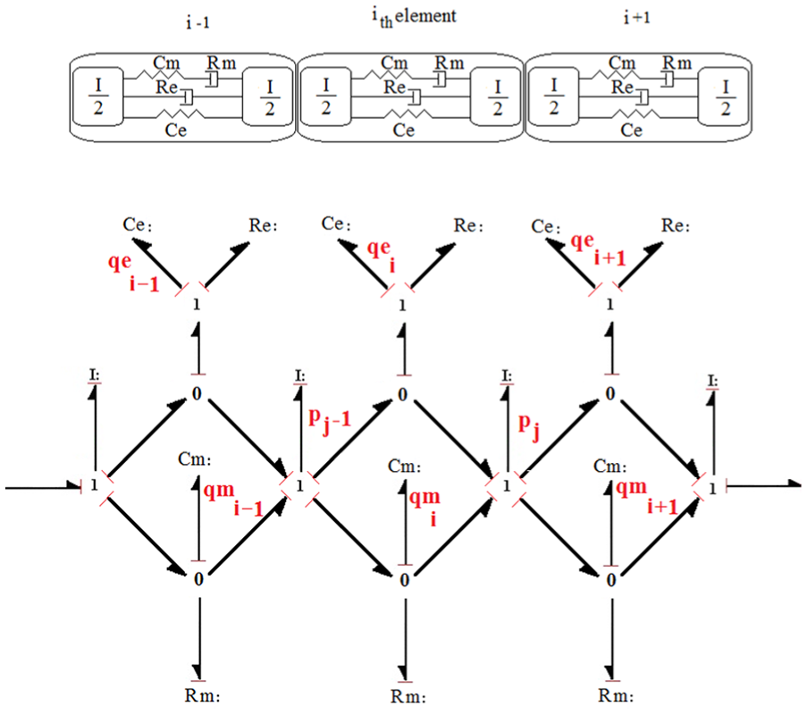
To define the energetic interaction between the involved subdomains of an elastic system, Rayleigh beam discrete geometry, suggested by Zanj and He, 23 is employed. Figure 3 shows a 1D distributed space on the basis of the acoustic assumption. According to this assumption, the elastic energy of the reticulated space can be stored in the center of each element and the movements of the boundaries are inertial. As this reticulated space is indeed a continuous system, the adjacent boundary of each two consecutive elements are bonded to move together. Therefore, one can consider the above discretization as a junction–element chain, in which each element represents the potential subdomain and each junction represents the kinetic subdomain, with its parameters being a weighted function of the related parameters of the adjacent elements.
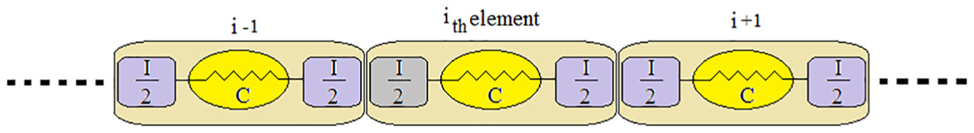
One-dimensional Rayleigh distributed geometry.
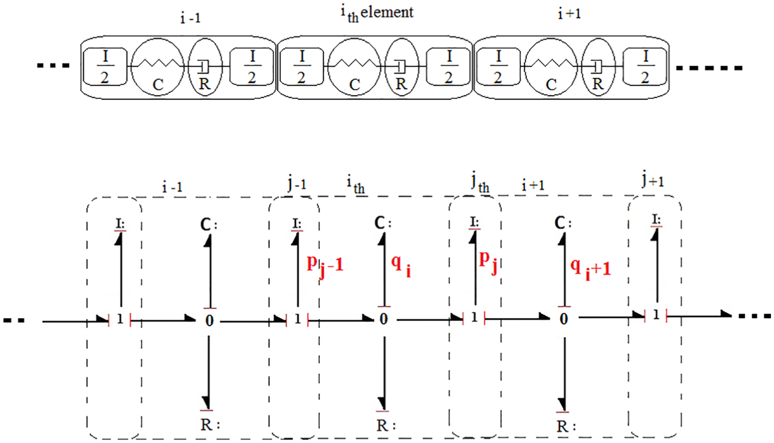
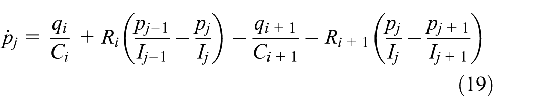
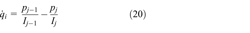
The BG representation of Figure 3 is shown in Figure 4. The considered state variables for the ith element and jth junction are
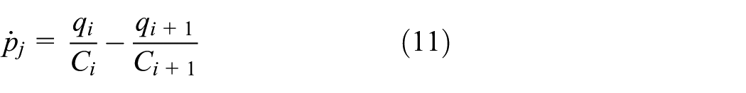

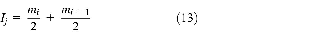
where
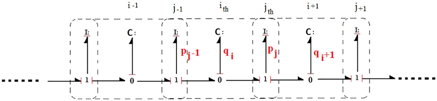
One-dimensional decomposed elastic model.
3.2. Domain-independent Maxwell viscoelastic model
Consider the series arrangement of the mechanical element in the Maxwell model shown in Figure 1(a). The relaxation mechanism embedded in this model can be interpreted as a dissipative component for the potential subdomain and placed in series with the capacity of each segment. The equivalent BG representation of the Maxwell model is presented in Figure 5, where a resistor is placed inside each element and in series with the storage element. This means that the internal energy of each medium can be saved or dissipated, resulting in a long-term stress release (creep) in the system.
Maxwell model bond graph representation of viscoelasticity.
For the BG model presented in Figure 5, the governing equations of the Maxwell model can be obtained as follows:
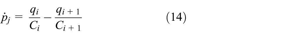
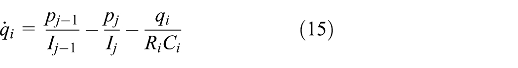
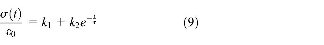
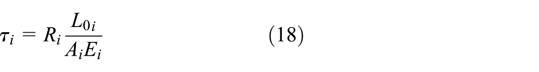
By integrating Equation (15) and comparing the result with the constitutive equation in Equation (9), the BG representation of the Maxwell relaxation time is equivalent to the following:

From the Hook’s relation for 1D reticulation, the storage coefficient is also presented as follows 23 :
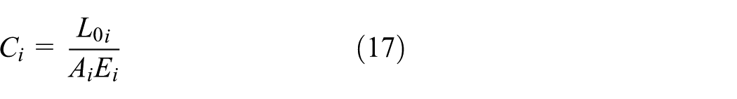
where
3.3. Domain-independent Kelvin–Voigt model
The Voigt model is well-known for systems under cyclic loading. As shown in Figure 1(b), the entropic dashpot of the Voigt model is placed in parallel with the main elasticity of the system. This model is known to capture the retardation behavior of the system. A BG representation of the Voigt model is given in Figure 6, where the energy entered into each medium is distributed between a resistor and a storage component with the same flow rate but different effort. This means that the system using the Voigt model can always conserve the internal potential energy without relaxing it.
Voigt model bond graph representation of viscoelasticity.
To extract the state equations of the Voigt model, by slightly changing the presented BG model to eliminate the existing loop, the BG presented in Figure 7 is suggested. Accordingly, the state equations for the ith segment and jth junction are derived as follows:
Loop-less Kelvin–Voigt model bond graph representation of viscoelasticity.
Comparing the Maxwell and Voigt BG models, one can notice that unlike the Maxwell model where the elastic energy of the system is dispersed, in the Voigt model the momentum energy of the system is dissipated as indicated by the causality of the resistive component. To explain this, consider the state equations of these two models. While the relaxation behavior in the Maxwell model occurs in the potential subdomain, the retardation behavior in the Voigt model occurs in the kinetic subdomain. This shows that these two viscoelastic models in fact describe two different phenomena occurring in different subdomains. Based on this finding, one can conclude that a combination of the Maxwell and Voigt methodologies is required to cover all the dissipation aspects of a real system.
3.4. Domain-independent SLS model
The SLS model attempts to include the dissipation impacts on both potential and kinetic subdomains; however, the obtained combination has a missing part. A Maxwell-like SLS BG model is presented in Figure 8, where a Maxwell arm is placed inside the system parallel to the main elasticity of the element. This allows the system to have a certain amount of relaxation and retardation.
Standard Linear Solid model bond graph representation of viscoelasticity.
As shown in Figure 8, an internal state is added to each segment. This added state temporarily stores elastic energy inside the segment, thus allowing the energy to relax to form creep-like dynamics. Define the added state,
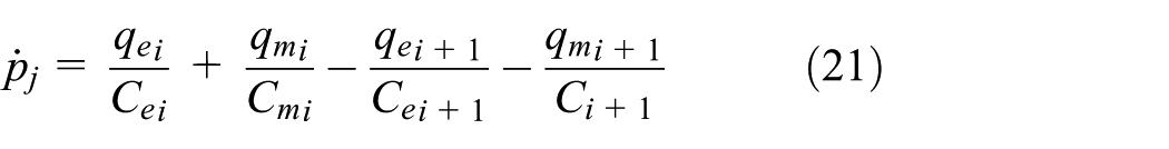

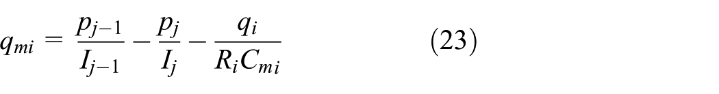
As can be seen, dissipative terms appear partially in the potential subdomain state equations (Equations (22) and (23)), but no direct viscoelastic impact is found in the kinetic subdomain state equation (Equation (21)). Although indirect viscoelastic impacts are shown in the kinetic subdomain via temporary forces generated in the system (the last two terms of Equation (21)), there is no sign of dispersion in the kinetic subdomain. This finding reveals that there is a missing part in the SLS model that will limit its performance in cyclic loading. It also explains the reason why there is little success in expanding the valid ranges of the SLS-like viscoelastic models even with the use of more complex means, such as the Weichert model shown in Figure 9. 12
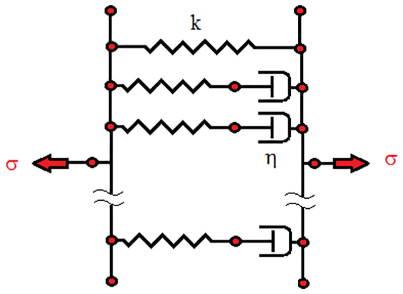
Weichert viscoelastic model.
3.5. Domain-independent Combined Linear Solid model
As has been seen, the BG technique can physically clarify the fundamental differences between relaxation and retardation mechanisms of a system using constructive components to form the viscoelastic behavior. Accordingly, to generate a complete model including all required dispersive mechanisms, a combination of the Maxwell and Voigt models is therefore proposed in which the direct dissipation can occur in both potential and kinetic subdomains. The proposed model is named the Combined Linear Solid (CLS) model, whose BG configuration is shown in Figure 10 where the simplest form of combining the Maxwell arms in parallel with the Voigt legs is presented.
Combined Linear Solid model bond graph representation of viscoelasticity.
Consider the index of
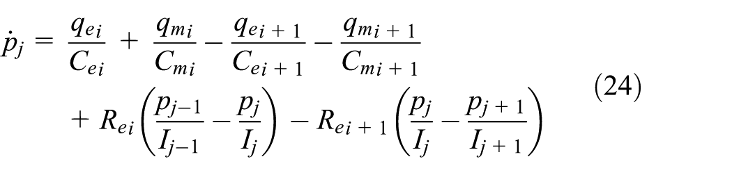
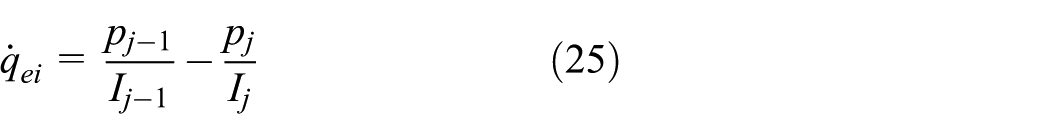
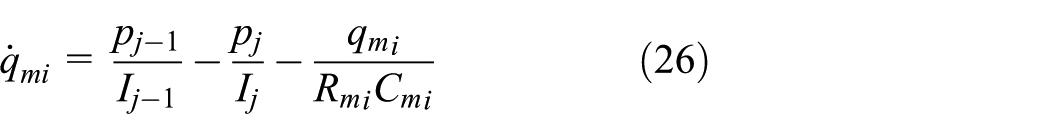
It is clear that, similar to the SLS model, the CLS configuration is also a three-degrees-of-freedom (3-DOF) system. The last two terms of Equation (24) indicate the direct dispersive impact on the kinetic subdomain, which include the retardation dynamics of the model. The last term in Equation (26) indicates the energy dissipation in the potential subdomain, which can be counted as the root of the long-term response of the system, including creep and relaxation dynamics. Unlike the SLS model, in the CLS model the energy transformation in both subdomains is dispersive, as demonstrated in Equations (24) and (26). Generating bidirectional attenuated dynamic interactions between the subdomains makes the CLS model capable of capturing the viscoelastic behavior of the system under high-frequency cyclic loading, where the SLS model fails to perform.
The physical interpretation of the existing dispersive mechanisms associated with the conventional methods has revealed that the dissipation of the system and the resultant viscoelastic behavior are the direct result of two phenomena occurring simultaneously inside different physical subdomains. These two phenomena are by nature different from each other. The difference between the orders of

It is clear that to obtain a logical relaxation time, in the kinetic subdomain the resistant coefficient is required to be of the order of the allocated mass of the segment, whereas in the potential subdomain the resistant coefficient is required to be defined of the order of the Young’s modulus of the segment. This fact highlights that the observed viscoelastic behavior of the system is indeed constructed by separate dynamic behaviors and, thus, separate parameters in different scales are required to regulate the model. The negligence of this fact in the conventional viscoelastic modeling techniques has resulted in divisions of models into two different categories: models suitable for long-term response and models suitable for cyclic loading. The consideration of separate relaxation time and retardation time, as shown in the proposed CLS model, however, can result in generating an integrated viscoelastic model suitable for all aspects of viscoelastic phenomena, and thus the CLS model has a much wider valid range.
3.6. Temperature dependency of viscoelasticity
Traditionally, to include the temperature dependency in the conventional models, the relaxation time is modulated via temperature input. In Section 2, it has been claimed that the consideration of relaxation time as a ratio of the viscosity coefficient to the Young’s modulus can limit the valid range of the conventional models and also can be the reason for some erroneous outcomes, especially in the presence of temperature fluctuations. To investigate this claim, in the following the physical interpretation of relaxation time modulation is highlighted via the energy-based modeling strategy.
To include the thermal subdomain influence on the elastic subdomain, consider the energy-based thermal model presented by Zanj and He 24 together with the CLS model, as shown in Figure 11. The dissipated energy is seen to enter into the thermal subdomain and change the temperature of the system via the RS energy links. Considering the energetic meaning of relaxation time, the modulation of this parameter can be presented as modulating its constructive components via the thermal information (signal lines shown as dashed lines in Figure 11) of the system. The modulation of resistance is permitted, as resistance is proportional to the instantaneous information (effort and flow) 14 of the system. However, the modulation of capacitance will undoubtedly violate the conservation of energy within the system, as capacitance is in an integrative relation with the instantaneous information of the system 13 and, thus, contains the memory of the model. To maintain the capacity conservation and at the same time to consider the temperature fluctuation, accompanied with the resistance modulation, a multi-dimensional thermoelastic capacitor 25 must replace the 1D capacitor in the model. This will include a different temperature-induced impact in the model than could be added by modulated resistance. Accordingly, one can clearly see how the implementation of a single modulation of relaxation time could result in disconnecting the model from the physical causality and thus neglecting a portion of the ongoing dynamic of the system, leading to a limited range of validity. According to the aforementioned facts, a complete consideration of the temperature dependency requires dynamic coupling between the anelastic domain and the thermal subdomain, which is beyond the scope of this study.
Possible thermal interaction of the viscoelastic model.
Given that the dissipated energy will transfer to the thermal subdomain via the bond shown in Figure 11, the amount of the dissipated energy can be obtained as follows:


where
This dissipated energy is another criterion reflecting the nature of the dispersive mechanism employed by the viscoelastic model. This criterion will be used in Section 4 as a comparative tool to highlight the fundamental differences between the proposed and the conventional dispersive mechanisms.
4. Simulation and result analysis
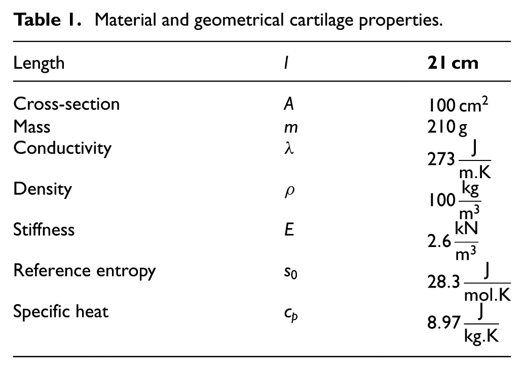
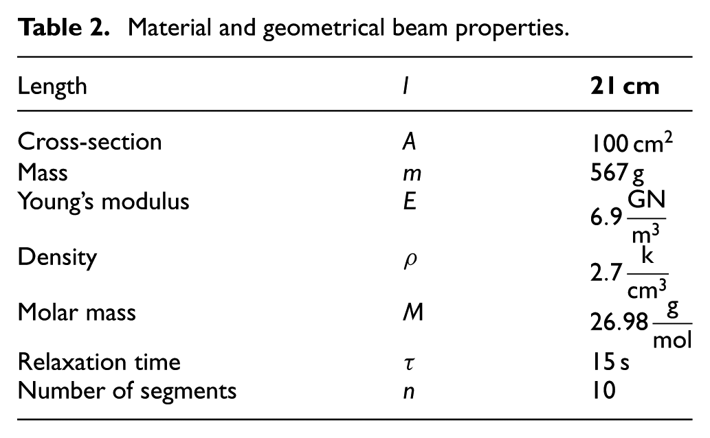
To compare the capability difference between the proposed CLS model and the conventional models in capturing viscoelastic phenomena, the axial behavior of a simple 1D discrete structure under cyclic loading is simulated using 20sim software. To generate the discretized geometry, the chosen structure is reticulated into 10 uniform elements with the first and last elements being the boundary elements that receive external mechanical controlled force as the boundary condition. It is assumed that all side surfaces of the structure are fully isolated and the system is stress-free initially at ambient room temperature. Sequentially, in Sections 4.1 and 4.2, the obtained results of the Maxwell and Voigt BG models shown in Figures 12–15 are compared for cyclic controlled tension of a soft material, the properties of which are listed in Table 1. In Sections 4.3 and 4.4, the obtained results of the SLS and CLS BG models shown in Figures 16–19 are compared for high- and low-frequency cyclic loading of a metallic alloy, the properties of which are listed in Table 2.
Beam viscoelastic behavior for soft materials.
Beam viscoelastic behavior for resistance altered soft materials.
Cartilage viscoelastic behavior under the Voigt model.
Maxwell (a) versus Voigt (b) under high-frequency loading.
Material and geometrical cartilage properties.
Deformation behavior under high-frequency loading, Standard Linear Solid approach (
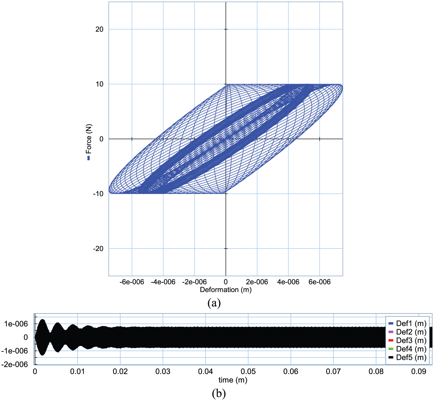
Combined Linear Solid model behavior under high-frequency loading (
Comparison between Standard Linear Solid (a) and Combined Linear Solid (b) models under high-frequency loading (
Combined Linear Solid model behavior under low-frequency loading for soft material (ω = 50 rad/s).
Material and geometrical beam properties.
4.1. Maxwell model
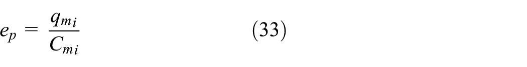
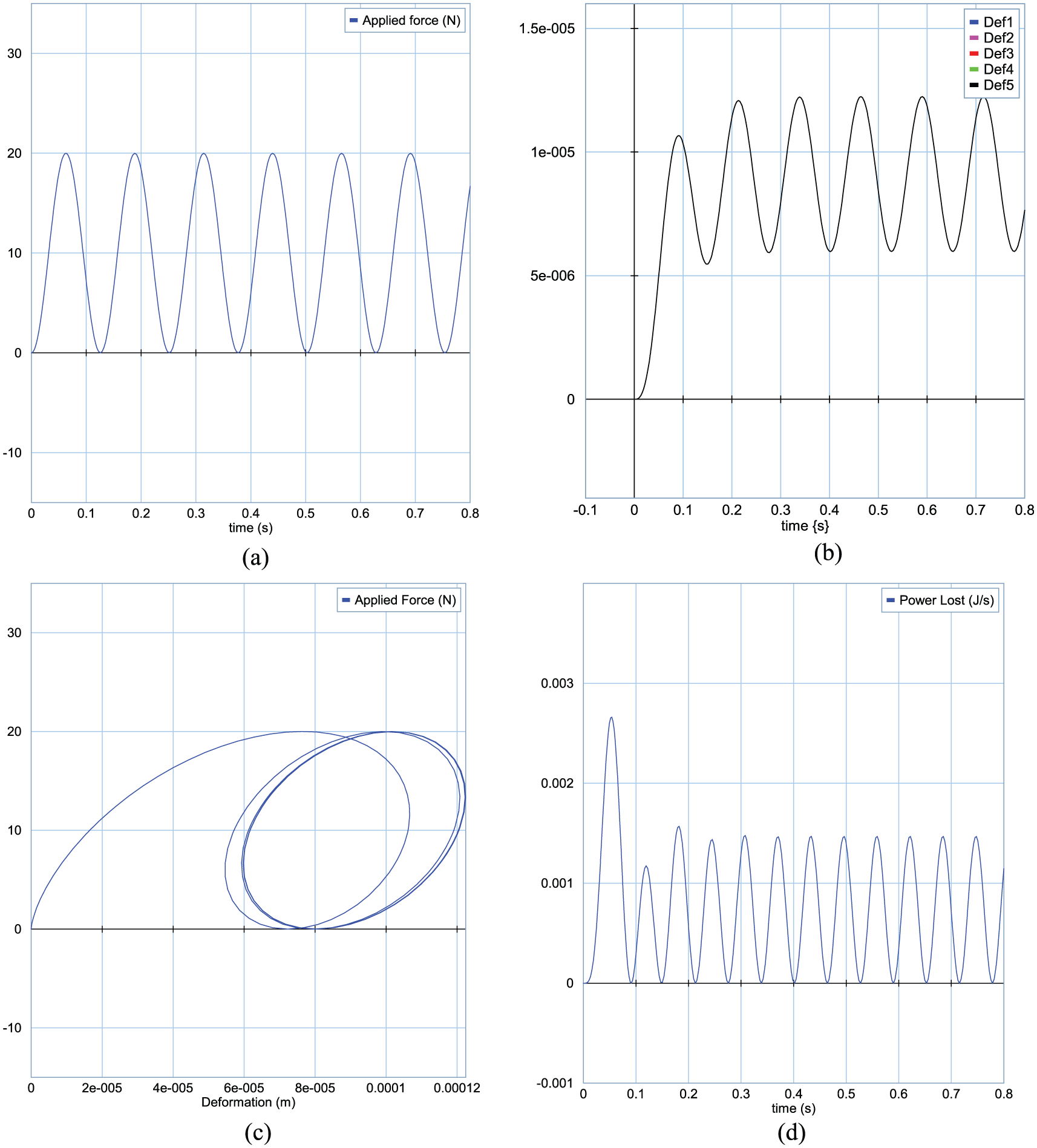
The results obtained from the Maxwell BG model of the system for the applied external force given in Figure 12(a) are presented in this section. The obtained deformation of each segment and the energetic behavior of the system are shown in Figures 12(b) and (c), respectively. They indicate the relaxation behavior of the system expected of the Maxwell model. For instance, the ratcheting of the system is clearly visible in Figure 12(c), which is one of the most desired behaviors in viscous materials. 26 The dissipated energy profile is shown in Figure 12(d). It can be concluded that the magnitude of the energy loss in the Maxwell dispersive model is considerable.
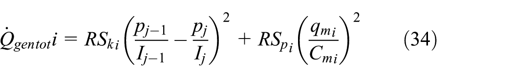
To physically identify the dispersive mechanism of the Maxwell model and to relate the considered dissipative coefficient with the material parameters, the resistance of the model is increased to the extent equal to the capacitance of the system. The obtained result for the same external force is depicted in Figure 13. Surprisingly, the deformation graph shown in Figure 13(b) demonstrates the elastic-like behavior of the system. In Figure 13(c), the energetic behavior of the system is reminiscent of Hooke’s force–deformation graph for elastic models. In Figure 13(d), the resultant dissipated energy of the system indicates that despite the increase in resistivity of the system, the amount of dissipated energy as compared to Figure 12(d) remains almost negligible. Collectively, one can conclude that in the Maxwell model increasing the resistivity leads to decreasing the viscoelasticity of the system.
To explain this conclusion from the model structure point of view, consider the Maxwell energetic component structure shown in Figure 5. According to this structure, the strain energy entering each segment (i.e., the considered flow traveling between the kinetic and potential subdomains) is seen to be free to select between the storage and the resistance components of the system. Similar to an electric circuit where the resistivity along the path of energy flow is high and there is a possibility to select between the resistor and the capacitor of the system, naturally the energy entering into the segment will be stored in the capacitor instead of being dissipated in the resistor. Thus, more pure elastic behavior is achievable with higher resistivity in the Maxwell model.
To explain this behavior from the material point of view, let us refer to the fundamental bases of domain-independent modeling. An outstanding advantage of the implemented energy-based method is that for any existing parameter in the model there must be a physical interpretation related to the material and geometrical entities of the system. In the case where the Maxwell resistance is altered, considering the observation of such elastic behavior, one could conclude that the Maxwell dispersive mechanism, appearing in the model as R, should in fact be related to the yield strength of that material. In other words, increasing this parameter in the model will change the material of the system from a soft material to a more brittle material. Or, in the case of a polymer, changes in R may be a representative of transferring from the viscous phase to the glassy phase due to temperature variation. This insight, in fact, could be considered as an outstanding capacity added to the BG representation of the Maxwell model for the process of parameter adjustment of the model, specifically in more complex situations.
4.2. Voigt model
To compare the Voigt model with the Maxwell model described above, in this section a similar energetic behavior of the system via the Voigt model is generated using the same loading situation and through changing the resistive parameter. Figure 14 shows the viscoelastic behavior of the system obtained from the Voigt model. The energetic behavior shown in Figure 14(c) is similar to that presented in Figure 13(c), but the internal dynamics presented in Figure 14(b) are different from those presented in Figure 13(b). It seems that the external dynamics of the Voigt model cannot find a way to enter into the system, whereas the deformation variation of different segments of the Maxwell model can vividly indicate the stimulated dynamics of the system. To explain this, examine the amount of the Voigt resistance (
From the explanation above, one can clearly ascertain that although the observable behaviors of the system in these two models are well-matched, their essences reflect two completely different physical dynamics of the system. These fundamental differences become more evident in high-frequency loading cases, especially when the models are under strain-rate control.
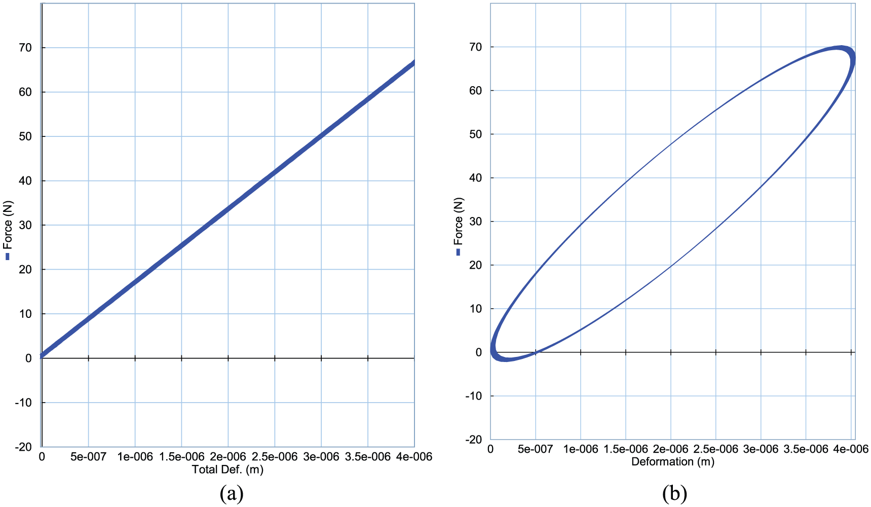
Figure 15 compares the force–deformation behaviors of the Maxwell (Figure 15(a)) and Voigt (Figure 15(b)) models for an aluminum alloy, described in Table 2, at higher frequency (
The comparison between the Maxwell and Voigt models indicates that these two models present two different aspects of the viscoelastic phenomena. Thus, both the Maxwell and Voigt dissipative mechanisms need to be included if all aspects of the viscoelastic behavior of a system are of concern. This fact can be considered as an introduction to generating a combined model, such as the SLS; however, the right combination still requires the right physical insight into the system.
4.3. SLS model
To evaluate the performance of the SLS model, a high-frequency force-control load (
4.4. CLS model
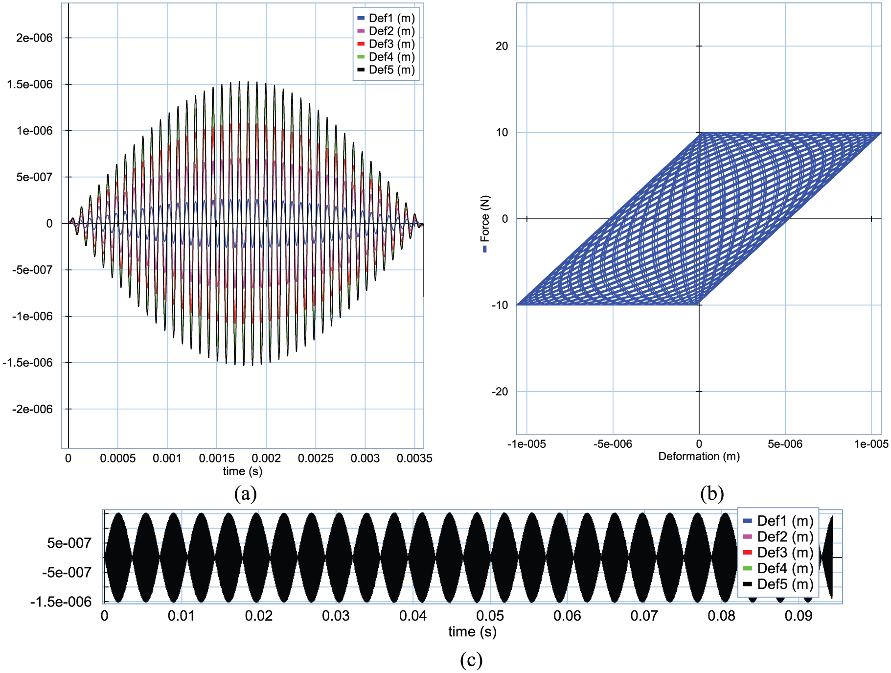
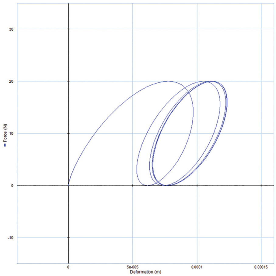
To examine the proposed CLS model, consider the same condition as applied to the SLS model. The obtained force–deformation of the CLS model is shown in Figure 17(a) where, in contrast to Figure 16(b), the damping behavior of the system is clearly demonstrated. As can be seen, after a finite number of oscillations, the dissipative mechanism embedded in the kinetic subdomain of the proposed CLS model drags the system out of the initial resonant mode and stabilizes the system into a new oscillatory condition.
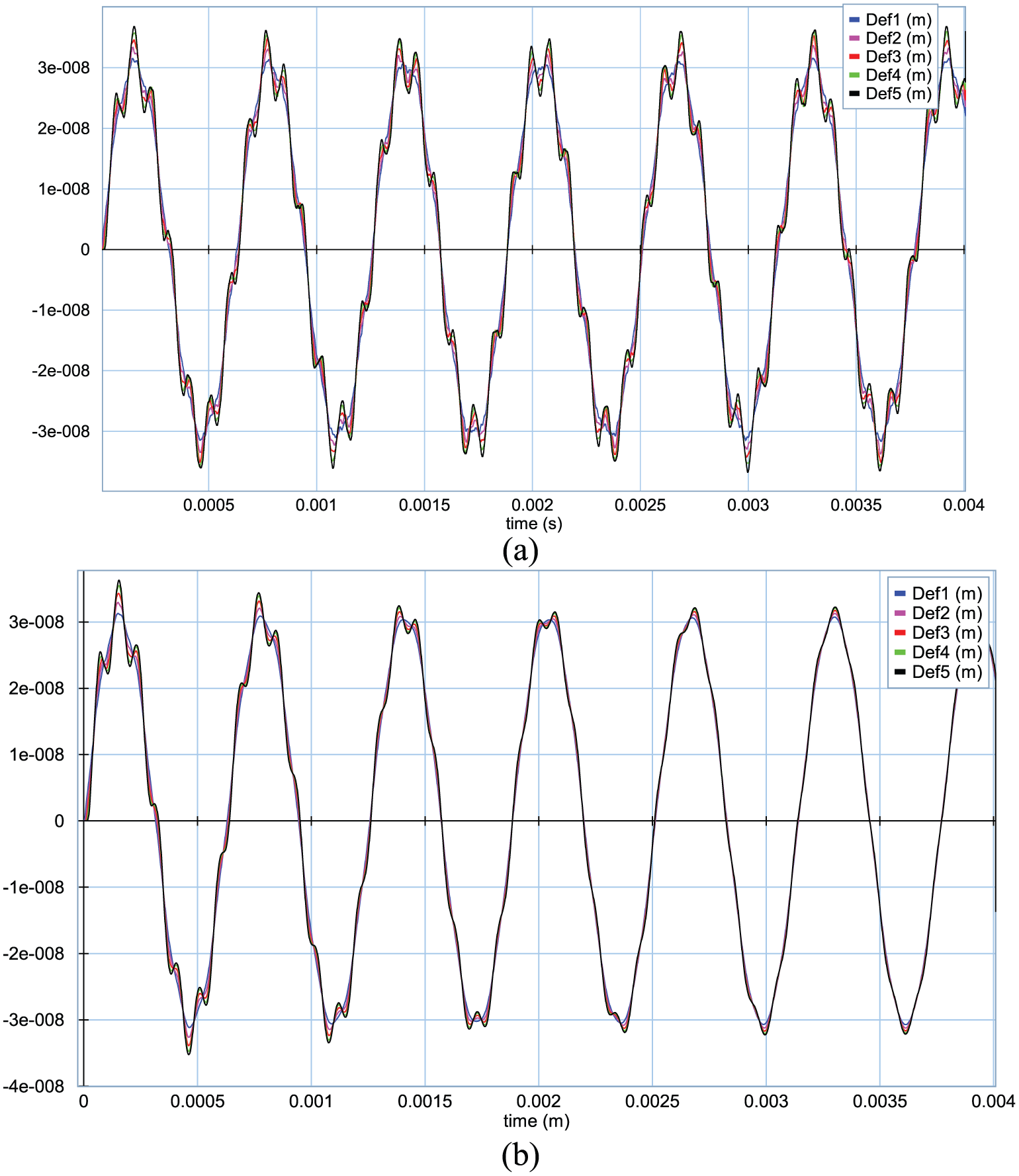
Figure 17(b) demonstrates the response of the system with respect to time. It is clear that some internal frequencies have totally vanished from the oscillation. To clarify the mechanism for this cancellation, closely examine the internal dynamics of the system at a lower frequency that is far enough from the natural frequency such that no resonance of the internal dynamics of the system could occur. A comparison between the obtained result from the SLS model shown in Figure 18(a) and that from the CLS model shown Figure 18(b) clarifies the significant role of the added dissipation mechanism to the kinetic subdomain of the proposed CLS model. One can see that in the CLS model, within each cycle of the oscillation the internally generated noise of the system is being dissipated, whereas in the SLS model no dissipation can be captured.
Having clarified that the CLS model offers better outputs at higher frequencies, the question of whether it can also perform well at lower frequencies may arise. To answer this question, a low-frequency situation, the same as that considered for the Maxwell model, is selected. Figure 19 presents the behavior of the system for the considered situation. As can be seen, the CLS model behavior is, to a good extent, comparable with that presented in Figure 12(c) for the Maxwell model. The graph indicates that in the low-frequency condition, the dissipative mechanism embedded inside the potential subdomain is dominant in forming the behavior, whereas the kinetic dispersive mechanism, although included, is not playing any key role.
Overall, the results indicate that having an insight into the arrangement of the common dissipative mechanisms respective to their involved physical subdomains may help in developing a single model that can cover a wider range of applications, as shown in Table 3. This single-model capability is greatly in demand for complex system dynamic investigations, such as in an aerothermoelastic analysis where an inclusive frequency spectrum is present and multi-physical domains are involved. Using a single model would be an advantage as it can lead to a significant reduction of solution cost during the system behavioral analysis.
Material and geometrical beam properties.
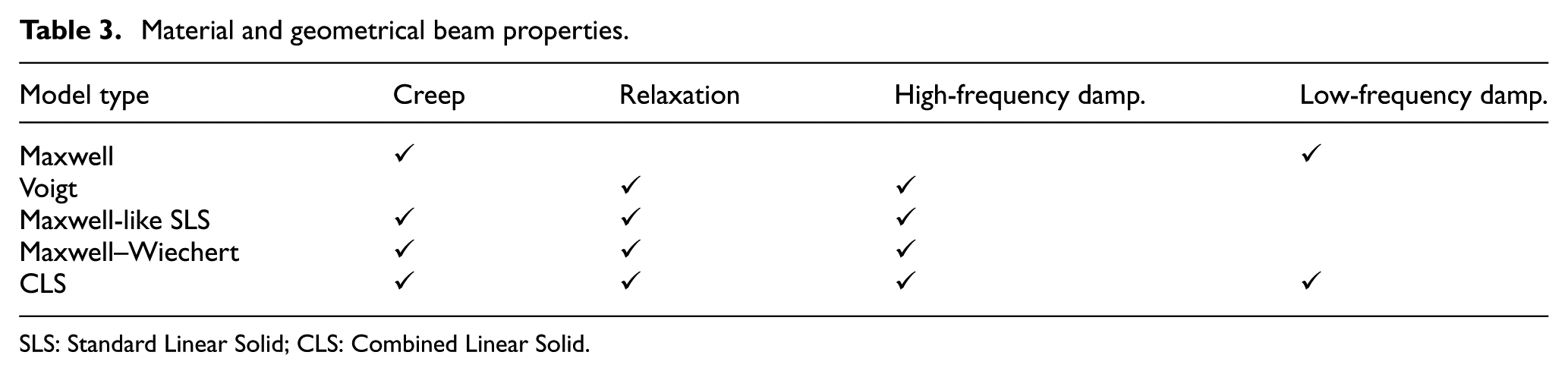
SLS: Standard Linear Solid; CLS: Combined Linear Solid.
In spite of all the advantages that a domain-independent model such as CLS can provide for a modeler, since the executed model introduces new parameters, identification and adjustment of such parameters may still be a matter of challenge for the modeler to address. However, the physical insight embedded in the proposed domain-independent modeling platform can be used as a guiding tool to define such parameters respective to the material and geometrical entities employed.
5. Conclusion
In this paper, by means of the BG approach, an energy-based combined viscoelastic model, namely the CLS model, is proposed based on the fusion of the conventional dispersive mechanisms. The comparison between the conventionally generated models and their BG representations indicates that the observable viscoelastic behavior of a system is in fact a direct result of two different dispersive mechanisms that act in two different physical subdomains of the system. Although both dispersive mechanisms result in energy dissipation, their impacts on the dynamics of the system are fundamentally different in different situations. Therefore, to describe the attenuation pattern of wave propagations in the system, both relaxation and retardation parameters are necessary for the whole range of frequencies. Furthermore, it is discovered that by employing the so-called relaxation time variable in the conventional viscoelastic models, the resistive and capacitive parameters of the system are combined in the system governing equations, which will limit the application of these models to a narrow range of fitted spectrum and single-domain dynamic investigations, while viscoelasticity solely is a multi-physical domain phenomenon, including the thermal subdomain.
By relating the viscoelastic behavior of a mechanical domain to the dissipation of its subdomains, a four-parameter CLS model is developed. The comparison between the obtained results indicates that although the mathematical interpretations of both the proposed model and the conventional SLS model are the same, there exists a significant difference between the performances of these two models. This highlights that in the CLS model the dynamic level in which the viscoelastic behavior of the system is formed is lower than that in the SLS model. Thus, more detailed interactions between the various subdomains of the system can be revealed in the CLS model in contrast to its conventional counterpart. With the use of the energy-based modeling technique, generating a model, such as the CLS, at the level of subdomains is entirely feasible. This feature has allowed the proposed CLS model to sufficiently reveal the impacts of the subdomain interactions and specialized dissipation mechanisms on forming the comprehensive viscoelastic behavior of the system.
Footnotes
Funding
This research received no specific grant from any funding agency in the public, commercial, or not-for-profit sectors.
Author biographies
![]()