A demonstration of using the model reference principle to develop the function-oriented adaptive pulse-coded neural network

Abstract

How can one design an adaptive pulsed neural network that is based on psycho-phenomenological foundations? In other words, how can one migrate the adaptive capability of a psychologically modeled neural network to a pulsed network? Neural networks that model psychological phenomena are at a larger scale than physiological models. There is a common presumption that pulse-coded neural network analogs to non-pulsing networks can be obtained by a simple mapping and scaling process of some sort. But the actual in vivo environment of pulse-coded neural network systems produces a much more diverse set of firing patterns. Thus, functional mapping from traditional neural network systems to pulse-coded neural network systems is much more challenging than has been presumed. This paper demonstrates that the employment of model reference adaptation as a method for applying scientific reduction is a powerful design tool for the development of a function-oriented adaptive pulse-coded neural network. The performance surface is empirically obtained by comparing the performance of the pulsed network to the non-pulsing network. Based on this surface, the adaptive algorithm is a combination of gain scheduling and steepest-descent method. Therefore, the adaptive property of the pulse-coded neural network is built upon a psycho-physiological foundation.

Keywords

Model reference principle adaptive pulse-coded neural network scientific reduction model-order reduction computational neuroscience embedding field theory

1. Introduction

The derivation of an adaptive pulse-coded neural networks (APCNN) model capable of demonstrating behavioral responses is the problem of interest for this paper. One may attempt to derive the APCNN using the bottom-up approach from individual Hodgkin–Huxley-like neurons. However, due to the current state of experimental art at the level of individual neurons, any psycho-physiological claim will lack objective validity. This is therefore not a trivial problem.

In this paper the above system problem is approached by using the model reference principle (MRP).¹ Although this is a powerful tool known to the systems engineer, to use this technique to bridge two different scales in neural network modeling is a novel approach. The MRP approach had been successfully implemented to identify the system.² That is, a pulse-coded neural networks (PCNN) structural analog to the reference model. However, unlike the reference model, this PCNN does not adapt. The subsequent question is therefore, how will the PCNN adapt? The paper tackles this problem by using the MRP.

Using the MRP, the adaptive response (behavior) of a level-coded (or activity-based) neural network is referenced to derive the APCNN (Figure 1). This means that the adaptive function is defined at the higher network system level, represented by the activity-based model. Hence, the derived APCNN is based on psycho-phenomenological foundations. Below is a discussion on why we chose the MRP.

Figure 1

Illustration of concept of model reference principle.

Phenomenological models are at a larger scale in comparison to biological models. They are therefore referred to as activity-based models. In the systems doctrine roadmap for theoretical neuroscience these psychological level models are models at a system level,² while the Hodgkin–Huxley-like models at the biological level perform component modeling.

The great majority of neurons in the brain have no direct contact with either sensory inputs or motor outputs. This makes it very difficult to understand what precisely the functional role of most small regions of neurons in central systems is. For instance, at the level of functional column structure in the neocortex, the neural networks contain thousands of individual neurons. With the current state of understanding in neuroscience and the current state of experimental art, individual probe implants or arrays of microbes are insufficient at this level of description. This paper demonstrates the derivation of an APCNN based on psycho-phenomenological foundations.

Through observable behavior and psychophysical correlates to behavior we can understand psychological phenomena. Migrating scientific study and theory from the level of phenomena more directly observable by our senses to levels of increasingly refined scientific constructs is called scientific reduction. Starting out from our understanding of behavioral responses we can use the method of dissection to penetrate it. For progress in penetrating nature the method of dissection has historically been shown to be better than abstraction,³ in our case, dissection from the adaptive level-coded neural network to the APCNN.

Using MRP, these different scaled models can be bridged. We therefore do not lose sight of the continuity of concepts and phenomena. This is consistent with Bacon’s investigative method. Bacon says the following³:

There are and can exist but two ways of investigating and discovering truth. The one hurries on rapidly from the senses and particulars to the most general axioms, and from them, as principles and their supposed indisputable truth, derives and discovers the intermediate axioms. This is the way now in use. The other constructs its axioms from the sense and particulars, by ascending continually and gradually, till it finally arrives at the most general axioms, which is the true but unattempted way.

2. Other work on PCNN

Most APCNNs are designed for engineering applications,⁴ many of which are in image processing. A number of these APCNNs use adaptive methods that implement mathematical trickery. For instance, to achieve a synchronized network for image segmentation the PCNN may be adapted by increasing the synaptic weight if the ‘membrane potential’ of the receiving neuron is behind the cycle and decreased otherwise.⁵

Outside image processing there has been some work on artificial systems and systems leaning toward neuroscience. Most of these works base their adaptation rule on the spike-time-dependent plasticity (STDP).^6-8 Spiking network structure that uses radial-basis function has been adapted using the learning windows of the temporal difference between the output neuron and input neuron for implementing STDP principle.⁶ STDP has also been carried out using exponential time-dependent weight change on leaky integrate-and-fire neurons (LIF) for spike-based machine learning.⁷ Some researchers have also coupled cerebellum biology-based networks to a robot,⁸ using the STDP-based bidirectional long-term plasticity rule to modulate output activity.

There have been other approaches, such as an LIF-based network adapting to expected timing of action-imperative stimuli.⁹ Connection weights are computed using the least-squares method, and the firing rate-based activity is interpreted as filtered spike trains. At the level of hardware, the STDP of artificial synapses has been implemented using metal-oxide memristors to store the weight values.¹⁰ The weights connecting the network of LIF units increase if the post-synaptic spike follows soon after a pre-synaptic spike, decrease if the opposite is true of the timing order, and are unaltered if the difference between spikes is small.

PCNNs designed with Eckhorn’s neural unit (ENU) produce wave-like firing action across the network (called autowaves) via its linking-field connection, with each network representing a pixel.^11,12 There are modified versions of ENU-based PCNNs. The self-adaptive autowave pulse-coupled neural network is an example.¹³ This was designed for the shortest path problem. Even some PCNNs that claim to be physiologically motivated,¹⁴ implement mathematical functions and techniques that diverge from biological plausibility. That is, they employs techniques or short-cuts to decrease the amount of computation for real-world engineering applications.

Before diving deep into the implementation of the MRP to derive the APCNN, the reference model (the higher-level model that can adapt) and the PCNN (the lower level model that we want to make adaptive) are described below. Implementing MRP in these models results in the performance surface, which is then used to design an adaptive algorithm. The algorithm is carried out to demonstrate the adaptation of the PCNN. Therefore, let us assume that we have a neural network model with some level of confidence and are interested in either scientific reduction or model-order reduction. That is, another neural network model of a different scale. This paper will show that the MRP is a powerful design tool for developing the model.

3. The Grossberg network

The adaptive resonance theory (ART) and its family of networks are often credited to Stephen Grossberg.^15,16 However, its key ideas were developed over a period of years.^17-21 Grossberg derived a nonlinear system of equations from simple psychological hypotheses. This is the fundamental principle of the embedding field theory.^18,20 The reference model used in this paper is from one of the early papers that laid the foundation for ART networks.²²

The reference Grossberg network (G-N) is an adaptive level-coded model that modulates or conditions sensory-motor acts (Figure 2). It was derived from the psychological postulates for the phenomena of punishment and avoidance. The model incorporates properties that produce positive and negative incentives for classical conditioning of sensory-motor acts. The psychological postulates are illustrated in Figure 2 and summarized as follows.

Figure 2.

Grossberg’s network (G-N). The dipole component (dipole network) is the part of G-N that receives input stimulus: tonic or bias, B and shock or drive, D. GD1 (Grossberg Dipole node 1) and GD2 respond to the stimulus with activities x₁ and x₂, respectively. At the second stage, GD3 and GD4 connected to GD1 and GD2 via elastic weights z₁ and z₂ and reinforced by the sensory (S) node via adaptive weights w₃ and w₄ responds with activities x₃ and x₄. At the third stage, GD5 with activity x₅ and GD6 with x₆ responds to excitation (x₃ and x₄, respectively) and mutual inhibition (dashed lines) between x₃ and x₄. Finally, their outputs O₅ and O₆ provide net-incentive motivation to the motor (M) node. Symbolically this is shown in Equations 1 and 2.

When a subject receives a shock (unconditioned stimulus, or drive, D) that induces fear, the subject experiences relief from fear of the shock immediately after the removal of shock stimulus (remaining tonic stimulus, or bias, B). These fear and relief responses form what Grossberg calls the net-incentive motivation. In addition, the generation of fear or relief response can be reinforced by another external stimulus (conditioning stimulus, or sensory, S). This learning of motivation patterns forms the reinforcement. This behavior of the network before conditioning/learning is illustrated in Figures 3(a) and 3(b). Its behavior during and after conditioning is shown in Figure 3(c) and 3(d), respectively.

Figure 3.

Behavior of G-N. (a and b) Plots of the behavior before conditioning/learning. The network receives a constant bias, B = 2. Addition of the drive input, D = 1 results in a response from the M-node (a). Prior to reinforcement when the network has not yet learned the conditioning stimulus (sensory, S = 0.8), its input does not produce a response (b). During conditioning, that is, when the S input is conditioned to the D input, the weights w₃ and w₄ undergo adaptation (c). After reinforcement, that is, when the network has learned the conditioning stimulus, its input produces a response (d).

The model is given by:

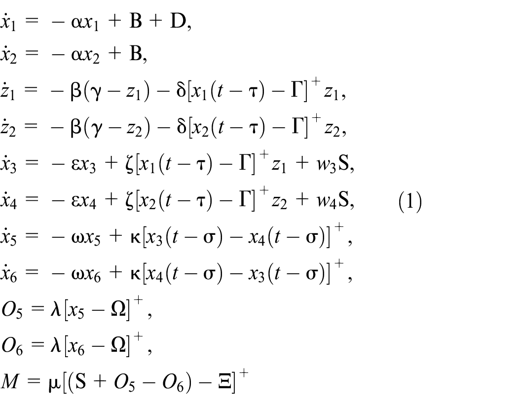
\begin{matrix} {\overset{\cdot}{x}}_{1} = - α x_{1} + B + D, \\ {\overset{\cdot}{x}}_{2} = - α x_{2} + B, \\ {\overset{\cdot}{z}}_{1} = - β (γ - z_{1}) - δ {[x_{1} (t - τ) - Γ]}^{+} z_{1}, \\ {\overset{\cdot}{z}}_{2} = - β (γ - z_{2}) - δ {[x_{2} (t - τ) - Γ]}^{+} z_{2}, \\ {\overset{\cdot}{x}}_{3} = - ε x_{3} + ζ {[x_{1} (t - τ) - Γ]}^{+} z_{1} + w_{3} S, \\ {\overset{\cdot}{x}}_{4} = - ε x_{4} + ζ {[x_{2} (t - τ) - Γ]}^{+} z_{2} + w_{4} S, \\ {\overset{\cdot}{x}}_{5} = - ω x_{5} + κ {[x_{3} (t - σ) - x_{4} (t - σ)]}^{+}, \\ {\overset{\cdot}{x}}_{6} = - ω x_{6} + κ {[x_{4} (t - σ) - x_{3} (t - σ)]}^{+}, \\ O_{5} = λ {[x_{5} - Ω]}^{+}, \\ O_{6} = λ {[x_{6} - Ω]}^{+}, \\ M = μ {[(S + O_{5} - O_{6}) - Ξ]}^{+} \end{matrix}

(1)

where parameters α = 3, β = 1, δ = 2/3, ε = ω = 3, ζ = 4/3, κ = 1, λ = 32, µ = 1, γ = 3, Δt = t−τ = t−σ = 0.01, Γ = 1/2, Ω = 0, Ξ = 1, bias B ∈ {2, 0}, unconditioned stimulus or drive D ∈ {1, 0}, and conditioning stimulus S ∈ {0.8, 0}. The Heaviside extractor [ y ]⁺ = max(y, 0) for any real number y. The rebound mechanism is due to z₁ and z₂; Grossberg calls them elastic weights. Thus, relief response occurs when shock (D) input (for fear) is removed.

The original G-N did not present a long-term adaptive function. Incorporating Grossberg’s outstar rule based on Hebb’s principle has been shown to make the G-N stably adaptive.²³ The weights (w₃ and w₄) with long-term adaptive capability is given by

\begin{matrix} {\overset{\cdot}{w}}_{3} = - ν_{3} w_{3} + η {[S - Γ_{S}]}^{+} {[x_{3} (t - τ) - Γ_{O}]}^{+}, \\ {\overset{\cdot}{w}}_{4} = - ν_{4} w_{4} + η {[S - Γ_{S}]}^{+} {[x_{4} (t - τ) - Γ_{O}]}^{+}, \\ ν_{3} = c {[S - Γ_{ν}]}^{+} + c' {[x_{1} (t - τ) - Γ_{ν'}]}^{+} {(S - Γ_{ν})}_{0}^{1}, \\ ν_{4} = c {[S - Γ_{ν}]}^{+} + c' {[x_{2} (t - τ) - Γ_{ν'}]}^{+} {(S - Γ_{ν})}_{0}^{1} \end{matrix}

(2)

where parameters η = 4.4, c = 0.03, c’ = 1, Γ_S = 0.5, Γ_O = 0.35, Γ_ν’ = 0.67, and Γ_ν = 0.79. ${(π)}_{0}^{1}$ is the unit step function. The presence of the very fast function ν_i causes the adaptive weight w_i to retain its values (i.e., learn). Note that we chose the sensory node output to be the conditioning stimulus (S).

4. The PCNN

The spiking network is composed of ENUs.²⁴ The pulsed network analog of the dipole component of G-N may be derived using the method of minimal anatomies.² In this paper a modified version of this network² is considered for the PCNN to be adapted. We call this the Eckhorn network (E-N, Figure 4).

Figure 4.

Eckhorn’s network (E-N). The neuromime pulse generator (NMPG) converts normalized dc-inputs; B, D, and S to pulsed-input. An EckX field may be composed of more than one sub-field. Eck1 has three sub-field: s₁, s_1modu, and s_1m-elas. A sub-field contains a variable number of ENUs (N). Sub-field s_1m-elas has N = 5, while field Eck3 has N = 2. Output from the individual ENUs of a particular sub-field form the elements of $\vec{Z}$ . Connections of one basic ENU (shaded) is shown for clarity. ∅ denotes adjustable weights, w₃ and w₄. The parts of a basic ENU are shown at the bottom. The symbolic description for the basic ENU is given in Equation 3. The parametric values for the E-N are given in Table 1.

Table 1.

Parameters for the Eckhorn dipole network (Figure 4).

	For: s_i, i ∈ {1, 2}		For: s_imodu, i ∈ {1, 2}		For: EckX, X ∈ {3, 4}
Parameters	B_Pulse	D_Pulse	B_Pulse	D_Pulse	S_Pulse
w	5	0.005	0.005	0.5	5
V_g	5	5	5	5	50
θ_O	0.5	0.5	0.5	0.5	0.5
τ_g	5	5	15	15	15

	For: EckX, X ∈ {1, 2}			For: EckX	For: EckX	For: EckM
Parameters	s_X	s_Xmodu	s_Xm-elas	X ∈ {3, 4}	X ∈ {5, 6}
N	5	5	5	2	2	1
w_l	0.5	0.5	0.5	0.5	0.5	0.5
τ_l	1	1	1	1	1	1
$w_{f}^{(+)}$	5	5	1	1.2	2.5	From S_Pulse: 5× 10⁻⁶
						From dipole: 2.5
$w_{f}^{(-)}$	-	-	0.5	-	5× 10⁻⁶	2.5
$τ_{f}^{(+)}$	10	10	10	10	10	10
$τ_{f}^{(-)}$	-	-	30	-	30	30
V_g	50	50	50	50	50	50
θ_O	0.5	0.5	0.5	0.5	0.5	0.5
τ_g	5	5	7.5	7.5	7.5	7.5

N = number of ENUs and step-size h = 1. Superscripts ⁽⁺⁾ and ⁽⁻⁾ are for excitatory and inhibitory connections, respectively.

The structural unit of the PCNN is the ENU. An individual ENU is given by:

\begin{matrix} F (t) = F (t - h) e^{\frac{- h}{τ_{f}}} + \frac{w_{f}}{τ_{f}} \sum_{\forall j} F_{j}^{inputs}, \\ L (t) = L (t - h) e^{\frac{- h}{τ_{l}}} + \frac{w_{l}}{τ_{l}} \sum_{\forall j} L_{j}^{inputs}, \end{matrix}

\begin{matrix} U_{i} (t) = F (t) (1 + L (t)), \\ V (t) = \sum_{\forall i} U_{i} (t), \\ θ_{V} (t + h) = {\begin{matrix} \begin{matrix} V_{g} & if V (t) ⩾ θ (t) \end{matrix} \\ \begin{matrix} θ_{V} (t) e^{\frac{- h}{τ_{g}}} & if V (t) < θ (t) \end{matrix} \end{matrix}, \\ θ (t) = θ_{O} + θ_{V} (t), \\ Z (t + h) = {\begin{matrix} \begin{matrix} 1 & if V (t) ⩾ θ (t) \end{matrix} \\ \begin{matrix} 0 & if V (t) < θ (t) \end{matrix} \end{matrix} \end{matrix}

(3)

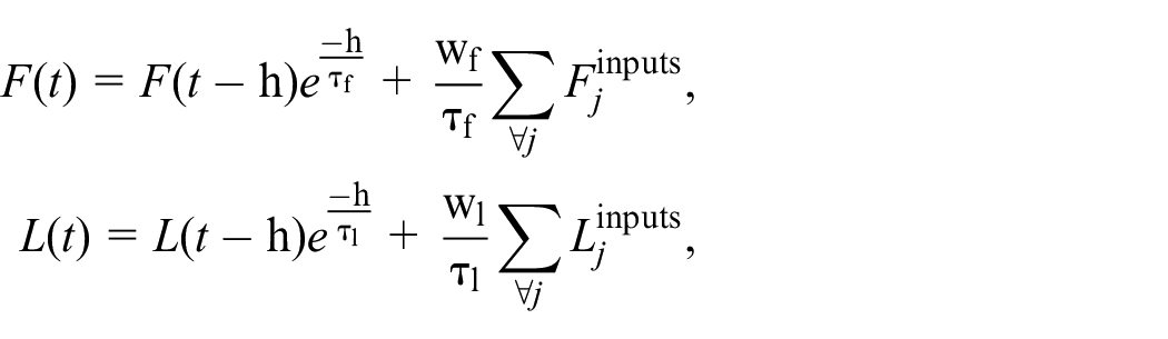
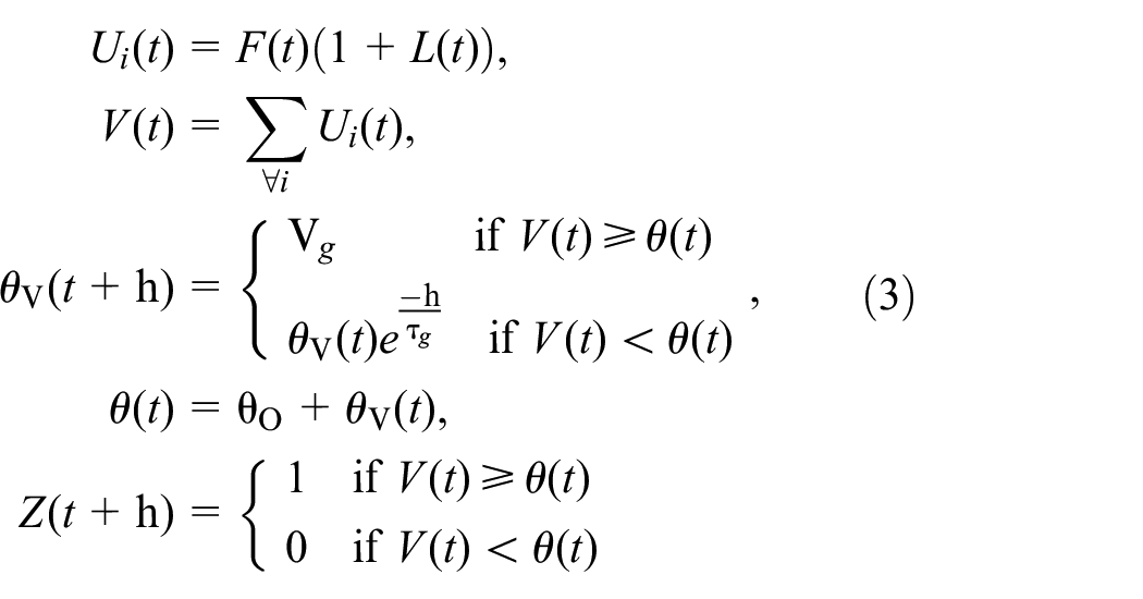
where τ_f, w_f, τ_l, w_l, V_g, τ_g, θ_O, and h are parameters.

The weights (w₃ and w₄) connecting the sensory input to the ENUs within Eck3 and Eck4 fields are adjustable. The feeding field output for the i^th ENU in Eck3 and Eck4 fields are given by:

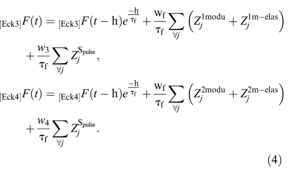
\begin{matrix} {}_{[Eck 3]}{F (t)} = {}_{[Eck 3]}{F (t - h)} e^{\frac{- h}{τ_{f}}} + \frac{w_{f}}{τ_{f}} \sum_{\forall j} (Z_{j}^{1 modu} + Z_{j}^{1 m - elas}) \\ + \frac{w_{3}}{τ_{f}} \sum_{\forall j} Z_{j}^{S_{pulse}}, \\ {}_{[Eck 4]}{F (t)} = {}_{[Eck 4]}{F (t - h)} e^{\frac{- h}{τ_{f}}} + \frac{w_{f}}{τ_{f}} \sum_{\forall j} (Z_{j}^{2 modu} + Z_{j}^{2 m - elas}) \\ + \frac{w_{4}}{τ_{f}} \sum_{\forall j} Z_{j}^{S_{pulse}} . \end{matrix}

(4)

The weights w₃ and w₄ will be the adapting weights for implementing the adaptation algorithm. The network behavior prior to learning is shown in Figure 5. MRP is employed by comparing E-N to the reference G-N to give us the performance surface.

Figure 5.

Behavior of E-N before conditioning/learning. The network receives a constant bias, B = 1. Addition of the drive input, D = 1, results in a response from the M-node (a). Prior to reinforcement when the network has not yet learned the conditioning stimulus (sensory, S = 1), its input does not produce a response (b).

5. The performance surface

Using MRP, the response of E-N is compared to that of G-N (Figure 6). We call this the model reference adaptation (MRA) approach. The two networks are of different signal types: real signal for G-N and spikes for E-N. Therefore, we must transform one of the signal types to compare them. In this paper the M-node spikes of E-N are transformed based on the method of moving point averages (MPA).^25,26 This is done as follows.

Figure 6.

Model reference adaptation (MRA) approach implemented for obtaining the error needed for measuring the performance of E-N.

Because activity levels are a product of multiple firings, let us consider a spike train with $K = \sum_{\forall i} i$ , inter-spike intervals (I_i). However, because of the difference in temporal scales, the transformed interval is T_i = I_i× 10⁻³ with an instantaneous firing rate R_i = T_i⁻¹. The number 10⁻³ comes from 1 ms ⇒ 10⁻³. The MPA is then:

MPA = \frac{\sum_{\forall i} R_{i}}{K + 1}

(5)

and the transformed spike train is as follows:

Z_{T} = k \times N \times MPA

(6)

where N is the number of ENUs in the field (or sub-field) and the constant of proportionality (k) can be determined such that error (d−Z_T) ≤ϵ, where d is the steady-state output value from G-N and ϵ is an arbitrarily small number. Here k = 0.5.

The performance surface is obtained with the E-N receiving B and S inputs but no D input. The surface is therefore also called conditioned performance surface. The performance index (P_Conditioned or P in short) is defined by:

P = {(d - Z_{T})}^{2}

(7)

the square of the difference between the transformed spike train (Z_T) and the desired steady-state output (d). This squared error is a measure of the performance of E-N relative to its reference, G-N. Thus, a smaller magnitude of P index reflects a smaller error and, therefore, better performance.

The performance of E-N is determined by manually changing w₃ and w₄ over a range of weight values. Following the scheme shown in Figure 6, the performance surface of the derived network is empirically obtained for individual adaptive weight pairs (w₃ & w₄).

Both w₃ and w₄∈ [0, 10] have Δw step. There will be $J = ⌊ (1 + Δ w) / Δ w ⌋$ numbers in [0, 10], where the floor $⌊ y ⌋ = y - (y mod 1)$ .

P is computed for J² weight pairs. For the fixed i^thw₃⁽ⁱ⁾ weight, the J weight pairs are: (w₃⁽ⁱ⁾ = 0, w₄⁽⁰⁾ = 0), (w₃⁽ⁱ⁾ = 0, w₄⁽¹⁾ = w₄⁽⁰⁾+Δw), …, (w₃⁽ⁱ⁾ = 0, w₄^{(J − 1)}= w₄^{(J − 2)}+Δw). There are J fixed w₃ weights, { w₃⁽⁰⁾, w₃⁽¹⁾, …, w₃⁽ⁱ⁾, …, w₃^(J-1) }.

Using the same Δw step, the performance landscape was obtained. Examination of this landscape showed good performances occurring in the weight range [4.5, 6.5]. Figure 7 shows the performance surface of the derived network, empirically obtained for individual adaptive weight pairs (w₃ and w₄) with weight step Δw = 0.1 for weight values between 4.5 and 6.5 and Δw = 0.25 elsewhere. Compute resource management was the reason for the difference in Δw.

Figure 7.

Conditioned performance surface of E-N. Shown below is the magnified 2-dimensional view along the w₃-axis of the 3-dimensional surface. It shows the region containing local minima and global minimum.

6. The adaptation algorithm

Following the empirically obtained performance surface in the preceding section the next step is to design the adaptation algorithm. Hence, the algorithm is based on the conditioned performance surface. Let us therefore study the performance surface (Figure 7).

Starting from initial weights (w₃⁽⁰⁾ = 0, w₄⁽⁰⁾ = 0), the surface is flat at maximum P, but with increasing weight values the surface has regions of local minima and a global minimum (arrows in Figure 7). The magnitudes of the minima values are however very close to each other (Figure 8). For instance, the difference between the global minimum and the largest local minima is of the order of 10⁻². Under the set membership paradigm for adaptive systems, these miniscule differences place the minimum points within the same solution set.^27,28 Further increase in weight values (w₃⁽ⁱ⁾ > 6.5, w₄⁽ⁱ⁾ > 5) results in the surface climbing, eventually reaching a maximum P (when w₄⁽ⁱ⁾ > 5).

Figure 8.

Semi-log scale of the 2-dimensional view of the conditioned performance surface seen in Figure 7.

Based on these observations, we consider the performance surface in terms of two regions: R1 or flat region and R2 or regions comprised of local and global minimum. The regions are identified by comparing the computed gradient, | Gradient | against a G_min. Steepest-descent method is then implemented around the region of minima while the principle of gain scheduling is implemented for performance outside the region of minima.

The two regions of the performance surface are distinguished based on the Gradient as follows:

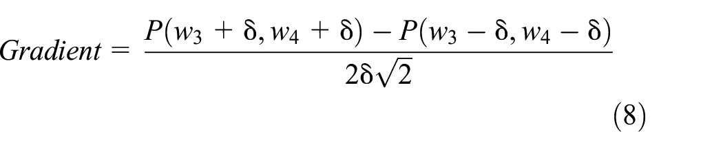
Gradient = \frac{P (w_{3} + δ, w_{4} + δ) - P (w_{3} - δ, w_{4} - δ)}{2 δ \sqrt{2}}

(8)

where δ = 0.005 and G_min = 0.05.

If the P of the network is in R1 of the surface, the weight is increased so that P is pushed like a hockey puck on the surface. In this push-weight procedure of gain scheduling:

{\vec{w}}_{j + 1} = {\vec{w}}_{j} + Pus h_{Uniform} + Pus h_{Extra}

(9)

where Push_Uniform= [0.04 0.04]^tr.

With just Push_Uniform the increasing adaptive weight due to the push could pass diagonally across the performance surface missing the region of minima. Therefore, the quantity Push_Extra is introduced. This quantity follows the Hebbian rule and is given by the following:

Pus h_{Extra} = [\begin{matrix} b {(Con n_{5, M} - Con n_{6, M})}_{0}^{1} \\ b {(Con n_{6, M} - Con n_{5, M})}_{0}^{1} \end{matrix}]

(10)

where b = 0.01 is the extra push parameter determined by the connection function Conn_i,M. The definition is as follows:

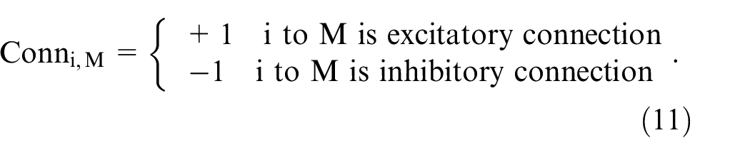
Con n_{i, M} = {\begin{matrix} \begin{matrix} + 1 & i to M is excitatory connection \end{matrix} \\ \begin{matrix} - 1 & i to M is inhibitory connection \end{matrix} \end{matrix} .

(11)

The adaptive w₃ weight is associated with the parallel sub-network where the connection between Eck5 and M-node is excitatory (Figure 4). Thus, Conn_5,M = +1. Similarly, Conn_6,M = −1. ${(y)}_{0}^{1}$ is the unit step function.

When the P of the network is in R2 of the surface, the updated weight is as follows:

{\vec{w}}_{j + 1} = {\vec{w}}_{j} + r \vec{\nabla}

(12)

with the rate of descent r = 5 × 10⁻⁶ and gradient

\vec{\nabla} = [\begin{matrix} \frac{P (w_{3} + δ) - P (w_{3} + δ)}{2 δ} \\ \frac{P (w_{4} + δ) - P (w_{4} + δ)}{2 δ} \end{matrix}]

(13)

with perturbation δ = 0.005. The adaptive weights cannot be negative. For the corner cases when either w₃ = 0 or w₄ = 0 (or both equals zero), the perturbation is one sided made only toward positive weights. Figure 9 shows the flowchart implementing the adaptive algorithm. The next section shows the experiments conducted on the PCNN.

Figure 9.

Flowchart of the adaptive algorithm for E-N. Note that during adaptation both P & P’ represent P_Conditioning.

7. Implementation of the algorithm

Learning occurs with the association of the conditioning stimulus (S) to the conditioned stimulus (D). That is, during adaptation E-N receives B, D, and S stimuli. Carrying out the algorithm with initial weights (w₃⁽⁰⁾ = 0, w₄⁽⁰⁾ = 0), the weight-learning curve is obtained (Figure 10(a)). Each progressive iterative step is associated with respective adaptive weights which result in a response from M-node. The calculated performance is called conditioning performance, P_Conditioning. As a result of the response from M-node, the calculated performance makes the conditioning learning curve move forward to the next iterative step (Figure 10(b)).

Figure 10.

Learning curves E-N. (a) Weight-learning curve plots the adaptive weights and (b) conditioning learning curve shows the performance index P (representing P_Conditioning) against iteration of the algorithm. (c) Illustration of the loop operation along the steepest-descent path and the dynamics of the learning curve in (d).

As described in the previous section, the adaptation algorithm is based on the conditioned performance surface (Figure 7). However, during the learning of the motivational process the network is being reinforced by the conditioning stimulus. This results in the conditioning performance surface (Figure 11). P_Conditioning is used for estimating the gradients (Figure 9). Therefore, the dynamics of the adapting weights depend on the conditioning surface, but the performance of the network with the adapted weights is evaluated against the conditioned surface.

Figure 11.

Conditioning performance surface of E-N. This is the performance surface of E-N receiving bias B, drive D, and sensory S (conditioning) stimuli. Shown below is the magnified 2-dimensional view along the w₃-axis of the 3-dimensional surface. Its shows the region containing local minima and global minimum.

The P (representing P_Conditioning) in the learning curve dips (arrow, Figure 10(b)) and then rises to a plateau (double arrow), but the difference between the least P and the value at plateau is of the order 10⁻². This apparent rise in P from the minimum P in the learning curve to its plateau, especially when considered with respect to the conditioned performance surface (P_Conditioned in Figure 11), becomes less significant. Thus, the minimum and plateau P values are within the solution set performance region in both performance surfaces as per set membership.

The basic essence of set membership theory or SMT (also called set-theoretic estimation)²⁷ is that a problem may have more than one mathematical solution (> 1 satisfactory point) such that any one of them when picked makes no practical difference. SMT produces a solution set whose characteristic is consistent with the observed data and available a priori knowledge. The estimate made by SMT is governed by the notion of feasibility, which is the solution set associated with the property set.

The gradient estimates show the dynamics of the learning curve (Figure 10(d)). During the first 99 iterations the gradient estimate for flat region check is | Gradient | ≤G_min = 0.05, thus adaptive weights follow the push-weight procedure (Figure 9). In later iterations, | Gradient | > G_min and the algorithm chooses the steepest-descent method. This causes ∇(w₃) to change (bottom trace) but ∇(w₄) remains at zero (not shown).

From around 170 iterative steps onward the gradient estimate for flat region check fluctuates due to ∇(w₃), though at different magnitudes (double arrow, Figure 10(d)). This ∇(w₃) fluctuation results in an average w₃ value (Figure 10(a)). The average w₃ (≈ 4.9056) and a non-changing w₄ (= 3.92) values causes the P plateau in the learning curve (double arrow, Figure 10(b)).

Therefore, the P plateau in the learning curve is due to the loop operation along the steepest-descent method path of the algorithm (Figure 10(c)). This is merely the usual misadjustment property of gradient descent.¹

8. Discussion

Level-coded models like the G-N and spiking models like the E-N are at different ends of the modeling scale. The models in the scale and the disciplines of an interdisciplinary field like the neuroscience may be thought of as the rungs of the neuroscience ladder. One way of connecting the rungs of the ladder is to migrate the scientific study and theory from the higher-level model to the lower-level model, that is, scientific reduction. For our particular problem the focus is on migrating the adaptive capability of the G-N to E-N. In this paper the scientific reduction is implemented using MRP.

The G-N and E-N models differ not only in scales (temporal resolution) but also in their signal types. Therefore, the PCNN pulse is transformed using MPA so that the outputs of the G-N and the E-N can be compared. Although seemingly obvious, most modeling in neuroscience takes this difference in signal types for granted when moving across different scales of models. MPA was chosen because of the variability of inter-spike intervals.

The application of this transformation procedure assumes that the ensemble firing frequency is proportional to functional neuroenergetics of the cortex.²⁹ Research on calibrating fMRI (Functional Magnetic Resonance Imaging) activities with electrical activities with respect to various neurotransmitter systems and brain regions is still an open field. In the future an accurate transformation process from a spiking-model neural network should have a stronger neurophysiological basis of fMRI.

With reference to the G-N output the performance of E-N is practically determined. The performance (P representing P_Conditioned) is measured on the presumption that the E-N is conditioned. The adaptable weights of the E-N is manually changed over a range of values. This conditioned performance surface is used to design the algorithm.

The performance surface is divided into two major regions: flat region (R1) and regions of local and global minima (R2). Depending on where P is on this surface, the weights are adjusted accordingly.

If P is in R1 the weights are adjusted by gain scheduling. The weights are pushed like a hockey puck by amounts Push_Uniform and Push_Extra. The problem of invoking Push_Extra and determining its parameter b is closely related to the ‘context-dependent choice’ problem.³⁰ That is, the same sensory cue can result in different responses depending upon the context. The connection types from the dipole network to M-node occur in complementary pairs.^31,32 Thus, if for a particular context the connection of dipole network channel (e.g., Eck1 → Eck3 → Eck5) with M-node is excitatory, then in another context the connection for the same channel may be inhibitory.

On the other hand, if P is in R2, the adaptation procedure switches to the steepest-descent method. Since the differences in magnitudes of P in the local and global minima are practically very small, from SMT we consider this to be the solution set performance region. Therefore, if the adjusted weights result in a P in this solution set region, we may say that the weights are adapted.

During the learning process of the PCNN the network is reinforced by the conditioning stimulus. Implementation of the algorithm results in learning curves of the weights and of the conditioning performance. At a given iteration the updated weights result in a performance index, P (representing P_Conditioning). The local and global minima of the conditioning performance surface falls within the solution set. Once the updated weights result in a corresponding P that lies in the solution set at the next iteration of the adaptation algorithm, P will lie within the solution set, but the value of P may or may not be equal. This is due to the gradient estimation noise, and the phenomenon is called the misadjustment property.¹

Because the network function is defined at the higher network level of G-N, the developed adaptive E-N is function-oriented. The adaptation in the APCNN is not ad hoc but by MRP. This makes the design process not lose sight of the continuity of concepts and phenomena. The four fundamental principles expressing the laws of continuity are³³:

a leap is not given in the sensible world (in mundo non datur saltus)

a gap is not given in the sensible world (in mundo non datur hiatus)

chance is not given in the sensible world (in mundo non datur casus)

fate is not given in the sensible world (in mundo non datur fatum).

The paper therefore demonstrates that the employment of the MRP adaptation technique is a powerful design tool for the development of function-oriented APCNNs. Although supervised learning is not new, the incorporation of the adaptive property of a large-scaled neural network with real signal into a smaller-scaled PCNN with spiking signal is novel. The design of the procedures comprising the adaptation algorithm is then based on the performance surface. Therefore, the design process does not lose sight of the continuity of phenomena. What is novel is not the APCNN, but how it was developed, that is, successfully using the MRP to bridge two different modeling scales.

Most current PCNNs in neuroscience follow analytic thinking. They are built on the assumption that the specific mechanisms learned from single cell studies also hold for networks. However, this is not justified for all mechanisms. For instance, specific mechanisms for potentiation in cell assemblies is still unclear. Synthetic thinking is the opposite of analytic thinking. It identifies the containing whole of the object of interest, explains the behavior of the whole and then disaggregates the explanation. The demonstrated design tool follows synthetic thinking. It provides the researcher with a tool for attempting to correlate the overall activity levels to observable potentiation effects in cell assemblies. It therefore does not saddle the researcher with a physical mechanism hypothesis while still trying to characterize the effects.

Supplemental Material

Instructions_to_run_the_codes – Supplemental material for A demonstration of using the model reference principle to develop the function-oriented adaptive pulse-coded neural network

Supplemental material, Instructions_to_run_the_codes for A demonstration of using the model reference principle to develop the function-oriented adaptive pulse-coded neural network by B Lungsi Sharma and Richard B Wells in SIMULATION

Footnotes

Funding

This work was supported by NIH Grant Number P20 RR016454 from the INBRE Program of the National Center for Research Resources.

Supplemental material

The codes for reproducing all the results are available at .

Author biographies

B Lungsi Sharma is a neuroscientist affiliated to the Ronin Institute and Centre national de la recherche scientifique, Gif-sur-Yvette. After receiving his medical degree from Kathmandu University in 2005, he got his Master of Science and PhD in neuroscience from the University of Idaho, Moscow, in 2011 and 2013, respectively. His main interest is modeling the mind-brain dynamic using scientific reduction and model-order reduction. He is a member of Sigma Xi and the National Council of Teachers of Mathematics.

Richard B Wells is Emeritus Professor of Electrical & Computer Engineering at the University of Idaho. He received his Bachelor of Science degree from Iowa State University, his Master of Science degree from Stanford University, and his PhD degree from the University of Idaho, all in Electrical Engineering. He served as the Associate Director of the MRC Institute and as the Director of the Program in Neuroscience, both at the University of Idaho. He also served as an Affiliate of the Department of Physiology and Biophysics at the University of Washington School of Medicine. He is a Senior Member of the Institute of Electrical & Electronic Engineers and served as an Adjunct Professor in the departments of Material Science & Engineering, the Program in Neuroscience, and Philosophy at the University of Idaho. He is a Life Member of Sigma Xi. He has served as Principal Investigator for numerous projects funded by the National Science Foundation and the US Department of Defense as well as for numerous research projects funded by the private sector.

References

Widrow

Stearns

. Adaptive signal processing. New Jersey: Prentice-Hall Inc., 1985.

Sharma

. Construction of a pulse-coupled dipole network capable of fear-like and relief-like responses. Connect Sci 2016; 28: 295-310.

Bacon

. Novum organum book I (new method). Translated by William

Wood

. Great Books Foundation series 1949. Chicago: Henry Regnery Company, 1620.

Wang

Cheng

, et al. Review of pulse-coupled neural networks. Image Vision Comput 2010; 28(1): 5-13.

Schreiter

Ramacher

Heittmann

, et al. Pulse coupled neural networks with adaptive synapses for image segmentation In: Lecture notes in informatics ARCS 2004: organic and pervasive computing, workshop proceedings (ed Brinkschulte

Becke

Fey

, et al.), 26 March 2004, P-41. Augsburg, Germany: GI, Gesellschaft für Informatik, Bonn, pp. 275-282. Retrieved from http://subs.emis.de/LNI/Proceedings/Proceedings41/article1167.html.

Wang

Belatreche

Maguire

, et al. An online supervised learning method for spiking neural networks with adaptive structure. Neurocomputing 2014; 144(20): 526-536.

Diehl

Cook

. Unsupervised learning of digit recognition using spike-timing-dependent plasticity. Front Comput Neurosci 2015; 9: 99.

Casellato

Antonietti

Garrido

, et al. Adaptive robotic control driven by a versatile spiking cerebellar network. PLoS One 2014; 9(11): 1-17.

Bekolay

Laubach

Eliasmith

. A spiking neural integrator model of the adaptive control of action by the medial prefrontal cortex. J Neurosci 2014; 34(5): 1892-1902.

10.

Prezioso

Merrikh Bayat

Hoskins

, et al. Self-adaptive spike-time-dependent plasticity of metal-oxide memristors. Sci Rep 2016; 6: 21331.

11.

Johnson

Ritter

. Observation of periodic waves in a pulse-coupled neural network. Opt Lett 1993; 18: 1253-1255.

12.

Johnson

. Pulse-coded neural networks: Translation, rotation, scale, distortion, and intensity signal invariance for images. Appl Opt 1994; 33: 6239-6253.

13.

Feng

. Self-adaptive autowave pulse-coupled neural network for shortest-path problem. Neurocomputing 2013; 115: 63-71.

14.

Broussard

. Physiologically-based vision modeling applications and gradient descent-based parameter adaptation of pulse coupled neural networks. Dissertation. Ohio: Air Force Institute of Technology, Wright-Patterson Air Force Base, USA, 1997.

15.

Grossberg

. Adaptive pattern classification and universal recoding I: parallel development and coding of neural feature detectors. Biol Cybern 1976; 23: 121–134.

16.

Grossberg

. Adaptive pattern classification and universal recoding II: feedback, expectations, olfaction, illusions. Biol Cybern 1976; 23: 187–202.

17.

Grossberg

. Some networks that can learn, remember, and reproduce any number of complicated space-time patterns I. Indiana University Math J 1969; 19: 53-91.

18.

Grossberg

. Embedding fields: A theory of learning with physiological implications. J Math Psychol 1969; 6: 209-239.

19.

Grossberg

. Some networks that can learn, remember, and reproduce any number of complicated space-time patterns, II. Studies in Applied Mathematics 1970; 49:135-166.

20.

Grossberg

. Embedding fields: underlying philosophy, mathematics, and applications to psychology, physiology, and anatomy. J Cybern 1971; 1: 28-50.

21.

Grossberg

. Contour enhancement, short term memory, and constancies in reverberating neural networks. Stud Appl Math 1973; 52: 213–257.

22.

Grossberg

. A neural theory of punishment and avoidance, II: Quantitative theory. Math Biosci 1972; 15: 253-285.

23.

Hill

Macpherson

Wells

. Affect-driven learning in an avalanche neural network modeling early sensorimotor intelligence. BMC Neurosci 2009; 10: 143.

24.

Eckhorn

Reitboeck

Arndt

, et al. Feature linking via synchronization among distributed assemblies: Simulations of results from cat visual cortex. Neural Comput 1990; 2: 293-307.

25.

Whittaker

Robinson

. Graduation, or the smoothing of data. In: The calculus of observations: a treatise on numerical mathematics. 4th ed. New York: Dover, 1967, pp. 65-156.

26.

Weisstein

. Moving average. MathWorld: A Wolfram Web Resource. http://mathworld.wolfram.com/MovingAverage.html (accessed February 5, 2011).

27.

Combettes

. The foundations of set theoretic estimation. Proc IEEE 1993; 81: 182-208.

28.

Zadeh

. On the definition of adaptivity. Proc IEEE 1963; 51: 469-470.

29.

Smith

Blumenfeld

Behar

, et al. Cerebral energetics and spiking frequency: the neurophysiological basis of fMRI. Proc Nat Acad Sci U S A 2002; 99(16): 10765-10770.

30.

Grossberg

. A theory of human memory: Self-organization and performance of sensory-motor codes, maps, and plans. In: Rosen

Snell

(eds) Progress in theoretical biology, Vol. 5. New York: Academic Press, 1978, pp. 233–374

31.

James

. The principles of psychology (in two volumes). New York: Dover Publications, 1890.

32.

Plutchik

. Emotion: a psychoevolutionary synthesis. New York: Harper & Row, 1980.

33.

Kant

. Lectures on metaphysics. Translated by Karl

Ameriks

Steve

Naragon

. Cambridge, UK: Cambridge University Press, 1997.

Supplementary Material

Please find the following supplemental material available below.

For Open Access articles published under a Creative Commons License, all supplemental material carries the same license as the article it is associated with.

For non-Open Access articles published, all supplemental material carries a non-exclusive license, and permission requests for re-use of supplemental material or any part of supplemental material shall be sent directly to the copyright owner as specified in the copyright notice associated with the article.

0.00 MB

0.40 MB