Sequential probability ratio tests: conservative and robust

Abstract

Because computers (except for parallel computers) generate simulation outputs sequentially, we recommend sequential probability ratio tests (SPRTs) for the statistical analysis of these outputs. However, until now simulation analysts have ignored SPRTs. To change this situation, we review SPRTs for the simplest case; namely, the case of choosing between two hypothesized values for the mean simulation output. For this case, the classic SPRT of Wald (Wald A. Sequential tests of statistical hypotheses. Ann Math Stat 1945; 16: 117–186) allows general types of distribution, including normal distributions with known variances. A modification permits unknown variances that are estimated. Hall (Hall WJ. Some sequential analogs of Stein’s two-stage test. Biometrika 1962; 49: 367–378) developed a SPRT that assumes normal distributions with unknown variances estimated from a pilot sample. A modification uses a fully sequential variance estimator. In this paper, we quantify the performance of the various SPRTs, using several Monte Carlo experiments. In experiment #1, simulation outputs are normal. Whereas Wald’s SPRT with estimated variance gives too high error rates, Hall’s original and modified SPRTs are “conservative”; that is, the actual error rates are smaller than those prespecified (nominal). Furthermore, our experiment shows that the most efficient SPRT is Hall’s modified SPRT. In experiment #2, we estimate the robustness of these SPRTs for non-normal output. For these two experiments, we provide details on their design and analysis; these details may also be useful for simulation experiments in general.

Keywords

Sequential test Wald Hall conservative robust

1. Introduction

While sequential probability ratio tests (SPRTs) are popular in application areas such as the testing of drugs on humans, they are virtually unknown in simulation. Indeed, testing drugs on humans should minimize the number of necessary observations, and SPRTs do so; that is, SPRTs are more efficient than classic tests such as the Student’s $t$ -test. In simulation, we should also strive for efficiency in the case where we need relatively much more computer time to obtain a single observation on the response (or output) of the given simulation model (this case is called “expensive simulation”). This need for efficient design and analysis of simulation experiments arises not only if we must choose between two hypothesized values for the mean simulation output (which is the focus of this paper), but also if we must choose among more than two simulated systems. Actually, the number of systems may be a given small number (e.g., 10), infinite (if continuous input variables define the system), or nearly infinite (if many discrete variables define the system). In these situations, we may try to estimate which system is optimal. This simulation optimization may use many statistical methods (see Kleijnen,¹ pp.241–300). However, until now these methods have not used SPRTs.

We point out that—unlike classic tests—SPRTs do not have a favorite null-hypothesis $H_{0}$ ; that is, classic tests reject $H_{0}$ only if there is strong counter-evidence that supports the alternative hypothesis $H_{1}$ . In practice, there may be good reasons for formulating a favorite hypothesis; for example, in criminal law this hypothesis stipulates that the accused is not guilty, and in management the current system may be replaced only if there is strong evidence that the proposed new system is better. However, if management is considering two new systems, then there may be no favorite $H_{0}$ .

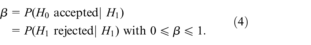
In mathematical statistics, it is well known that SPRTs are more effective in the sense that SPRTs control both the type-I or $α$ error probability—defined as $P (H_{0}$ rejected | $H_{0}$ )—and the type-II or $β$ error probability— $P (H_{0}$ accepted | $H_{1}$ ). However, SPRTs are not mentioned at all in the most popular simulation textbook; namely (Law²). Therefore, we provide a gentle introduction to SPRTs for the simulation community. We focus this review on random simulation, which includes discrete-event simulation (DES) and agent-based simulation (ABS); continuous simulation uses differential or difference equations, and is usually deterministic. Both deterministic simulation and random simulation may have inputs with unknown values, so probability density functions (PDFs) are used to “propagate uncertainty through the model”; this propagation is called risk analysis or uncertainty analysis. Whenever the simulation involves random inputs, the output (response) becomes random too.¹

Mathematically speaking, the simulation output is a complicated implicit function of the inputs, including the pseudorandom number (PRN) stream determined by the PRN “seed” or initial value. This randomness implies that we must decide how many observations we want to obtain on the output, in order to obtain a “precise” estimate of the true output. To make such a decision, we should use statistical methods. The selection of these methods varies with the problem that we try to solve through the simulation model. In this paper, we focus on the simplest problem; namely, the simulation output is an estimate of the mean (say) $μ$ for a given input combination. To illustrate this problem, we consider the following example (also see footnote ²).

Suppose management is interested in the following two system variants. System 1 is supposed to have a mean output $μ$ = 100 (e.g., 100 pieces of throughput), and system 2 has a mean output that is 10% higher; so, $H_{0}$ : $μ$ = 100 and $H_{1}$ : $μ$ = 110. The simulation analysts build models of the two systems. Next the analysts must decide whether they have collected enough simulated observations to conclude whether $H_{0}$ or $H_{1}$ holds. The analysts may then apply a SPRT.

We claim that SPRTs may be useful in simulation, because most computer systems proceed sequentially. For example, a 1975 textbook on simulation (Kleijnen,³ pp.503–505) has already discussed the SPRT originally developed by Wald.⁴ A recent publication on SPRTs is the book on sequential statistics by Govindarajulu,⁵ which we shall use repeatedly in this paper. In the next sections we define Wald’s⁴ SPRT, Hall’s⁶ SPRT, and our simple heuristic modifications of these SPRTs. Hall⁶ (p.376) proposes similar modifications, stating: “No theoretical evaluation of these procedures has been possible.” Hall⁶ (Chapter 2) anticipates our modification of Wald’s SPRT. In this paper, we explain the dynamic behavior of these SPRTs. We also quantify the performance of these SPRTs, using several Monte Carlo (MC) experiments with prespecified nominal $α$ and $β$ error probabilities and prespecified distance between the parameter values in $H_{0}$ or $H_{1}$ . Note that we use the term MC for models that use PRNs, whereas we use the term simulation for dynamic models, which may be either random (so they are a type of MC) or deterministic. We carefully design these MC experiments including classic factorial designs and our modified central composite design (CCD) (instead of one-factor-at-a-time designs, which are often used in current simulation experiments), a carefully selected number of (macro)replications, and use of common random numbers (CRNs). Moreover, we analyze the experimental results through regression analysis that quantifies the interactions among experimental factors and the marginal effects of these factors; this analysis distinguishes between “per comparison” error rates and “familywise” error rates. (Our design and analysis may also be used in simulation experiments, in general.) ⁴

The seminal article by Wald⁴ assumes that the output (say) $x$ has an explicit probability density function (PDF) with a single parameter $θ$ . This assumption holds for exponential distributions, normal (or Gaussian) distributions with known standard deviations, etc. Next, Hall⁶ assumes that the PDF is normal so $x ~ N (μ_{x}, σ_{x})$ , where $μ_{x} = μ_{0}$ in $H_{0}$ and $μ_{x} = μ_{1}$ in $H_{1}$ , and $σ_{x}$ is unknown and is estimated from a pilot sample; in the rest of our paper we suppress the subscript $x$ if the context shows which random variable is meant. Wald⁴ (pp.132–133) and Hall⁶ (p.369) mention that the resulting SPRTs are conservative, that is, the actual error rates are smaller than the prespecified or “nominal” values (so, these values could have been realized with fewer observations than the SPRTs actually require). In this paper, we quantify the degree of conservativeness. Moreover, we investigate the robustness of these SPRTs; that is, we quantify the sensitivity of the SPRTs to non-normality if the analysts actually assume normality. In simulation practice, the output may indeed be non-normal.⁵ For example, Kleijnen¹ (p.92) reports that the estimated average and the estimated 90% quantile of the output of a simulated queueing model (namely, a so-called M/M/1 model) are not normally distributed if the simulation run has only 1,000 simulated arrivals and the traffic rates are 0.5 and 0.9, respectively. In practice we often do not know which type of distribution the output has, so it is important to investigate the robustness of SPRTs.

We organize the rest of our paper as follows. In Section 2 we present details on Wald’s⁴ and Hall’s⁶ SPRTs, including simple modifications. In Section 3 we quantify the performance of these SPRTs in experiment #1, guaranteeing that the output is indeed normally distributed. In Section 3.1 we present details on the design of this experiment; in Section 3.2 we detail the analysis of the results of this experiment. This experiment suggests that Wald’s⁴ SPRT with estimated variance gives significantly high error rates, and that Hall’s⁶ SPRTs are conservative; the most efficient SPRT is the modified Hall⁶ SPRT. In Section 4 we detail experiment #2, which suggests that the SPRTs are robust. In Section 5 we present conclusions, and mention future research topics.

2. Overview of Wald’s and Hall’s sequential probability ratio tests

In this section we define Wald’s⁴ SPRT and Hall’s⁶ SPRT, plus simple modifications of these SPRTs. Moreover, we add some comments because these SPRTs differ from the classic test using $t$ -statistic and $p$ -values.

2.1. Wald’s SPRT

Wald⁴ assumes a sequence of $n$ independent and identically distributed (IID) observations $x_{i} (i = 1, \dots, n)$ on the random variable $x$ with the PDF $f (x | μ)$ , where $μ = E (x)$ and:

H_{0} : μ = h_{0} versus H_{1} : μ = h_{1},

(1)

where $h_{0}$ and $h_{1}$ denote values specified by the users. An example is a normal PDF with mean $μ$ and known variance. We use Greek lower-case letters to denote a parameter, which by definition has a value that is inferred from data such as $x_{i}$ (see the fundamental simulation textbook Zeigler et al. In a simulation context, $x_{i}$ may represent the output of simulation replication $i$ ; by definition, replications give IID observations. As is traditional, we use a “hat” to denote estimates (e.g., $\hat{μ}$ ) and a “bar” to denote sample averages (e.g., $\bar{x}$ ). A list of abbreviations and major mathematical symbols with their definitions is given in Appendix 2.

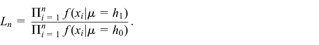
By definition, the “probability ratio” (in the term “SPRT”)—also called the likelihood ratio (say) $L$ —of $x_{i}$ with $i = 1, \dots, n$ is as follows:

L_{n} = \frac{Π_{i = 1}^{n} f (x_{i} | μ = h_{1})}{Π_{i = 1}^{n} f (x_{i} | μ = h_{0})} .

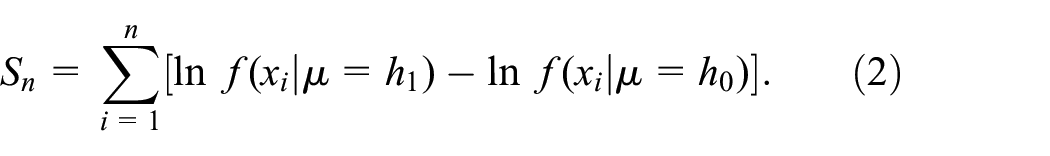
It is convenient to apply the logarithmic transformation to this $L_{n}$ , which leads to the test statistic as follows:

S_{n} = \sum_{i = 1}^{n} [\ln f (x_{i} | μ = h_{1}) - \ln f (x_{i} | μ = h_{0})] .

(2)

Intuitively, we accept $H_{0}$ if $S_{n}$ is “low,” whereas we accept $H_{1}$ if $S_{n}$ is “high.” The classic error probabilities $α$ and $β$ (type-I and type-II error probabilities) are as follows:

\begin{matrix} α = P (H_{0} rejected | H_{0}) \\ = P (H_{1} accepted | H_{0}) with 0 \leq α \leq 1, \end{matrix}

(3)

\begin{matrix} β = P (H_{0} accepted | H_{1}) \\ = P (H_{1} rejected | H_{1}) with 0 \leq β \leq 1 . \end{matrix}

(4)

The SPRT treats $H_{0}$ and $H_{1}$ similarly, whereas classic tests “favor” $H_{0}$ . An example of such a classic test is the $t$ -test (also see Equation (17) below). Classic tests control $α$ , whereas $β$ may be computed—given the sample size $n$ and the difference $| h_{0} - h_{1} |$ (also see Law,² (pp.560–565)). We let $A$ and $B$ denote the nominal values prespecified for $α$ and $β$ , respectively. Then this SPRT has the following decision rule:

Accept H_{0} if S_{n} \leq \ln \frac{B}{1 - A},

(5)

accept H_{1} if S_{n} \geq \ln \frac{1 - B}{A};

(6)

else, obtain x_{n + 1}, and compute S_{n + 1} .

(7)

We implement various SPRTs in MATLAB software, using Govindarajulu⁵ (Section 6.2.1), but we correct some errors in this software for the SPRT due to Hall⁶ (p.369); see the next section. Actually, Wald’s SPRT is conservative: $α < A$ and $β < B$ (see Wald⁴ (pp.132–133) and Hall⁶ (p.369)). We shall estimate the magnitudes of $A - α$ and $B - β$ using the extensive MC experiment in Section 3.

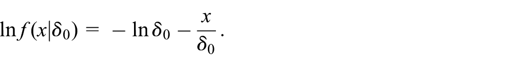
To illustrate the computation of $S_{n}$ defined in Equation (2), we use the exponential PDF and the normal PDF (which we also use in later sections). The exponential PDF with parameter $δ$ —which we denote by expo $(δ)$ —is $f (x | δ) = δ^{- 1} e^{- x / δ}$ if $x > 0$ ; else 0 (in Equation (1) we use the general symbol $μ$ instead of the specific symbol $δ$ ). To compute $S_{n}$ , we need the following:

\ln f (x | δ_{0}) = - \ln δ_{0} - \frac{x}{δ_{0}} .

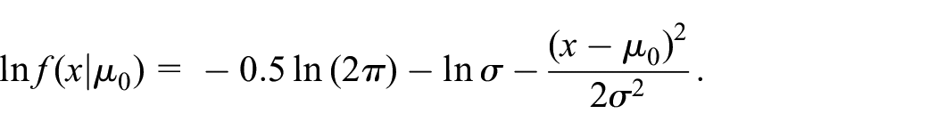
The normal PDF is $f (x | μ, σ) = (2 σ^{2} π)^{- 1 / 2} \exp (- (x - μ)^{2} / (2 σ^{2}))$ . Because Wald⁴ assumes that $σ$ is known, this PDF gives the following:

\ln f (x | μ_{0}) = - 0.5 \ln (2 π) - \ln σ - \frac{{(x - μ_{0})}^{2}}{2 σ^{2}} .

We, however, either follow Hall⁶ and estimate $σ^{2}$ through $s_{m}^{2}$ —the classic variance estimator with a fixed (pilot) sample size $m$ —or use the modified Hall⁶ SPRT with $σ^{2}$ estimated sequentially through $s_{n}^{2}$ (see Section 2.2).

Now we illustrate the behavior of this SPRT, giving examples with the extreme (unrealistic) values $B$ = 0 and $A$ = 0, respectively. If $B$ = 0, then Equation (5) gives $\ln [B / (1 - A)] = \ln 0 = - \infty$ so $H_{0}$ is never accepted; that is, $H_{1}$ is always accepted so we never reject $H_{1}$ falsely. If $A$ = 0, then Equation (6) gives $\ln [(1 - B) / A] = \ln \infty = \infty$ so $H_{1}$ is never accepted; that is, $H_{0}$ is always accepted so we never reject $H_{0}$ falsely.

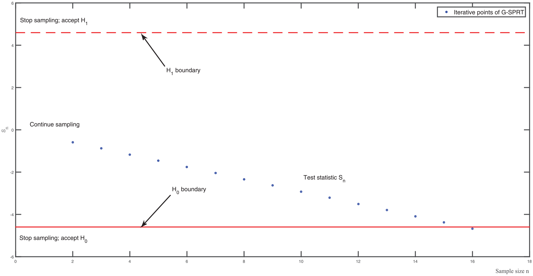
Even though the SPRT does not have a favorite hypothesis, we may treat $H_{0}$ and $H_{1}$ differently because the consequences of erroneously rejecting $H_{0}$ or $H_{1}$ may be different in practice.⁷) We may then select different values for $A$ and $B$ . If $A$ $\neq B$ , then the two boundaries defined in the right-hand sides of Equations (5) and (6) are not at equal distances from the origin, which is the point (0, 0) (see Figure 1, discussed next).

Figure 1.

Example boundaries and sample path for Wald’s sequential probability ratio test with $x ~ N (0, 1)$ , $s_{n}^{2}$ , $h_{0}$ = 0, $h_{1} = 0.5$ , $A = 0.01, B = 0.01$ .

Equations (5) and (6) imply that the sample path of $S_{n}$ stops when $S_{n}$ crosses one of the two boundaries. Figure 1 gives an example in which the SPRT stops when $S_{n}$ crosses the lower boundary at the final sample size $n_{f}$ = 16; the SPRT then accepts $H_{0}$ . So, $n_{f}$ depends on the sample path of $S_{n}$ and the size of the continuation region between the two boundaries, which is determined by the prespecified values $A$ and $B$ . A larger value of $A$ and $B$ (e.g., 0.10 instead of 0.01) narrows this region, and thus tends to decrease $n_{f}$ . More specifically, as $A$ increases, the upper boundary decreases, so $S_{n}$ crosses this boundary more quickly and accepts $H_{1}$ ; that is, the SPRT gives a smaller $n_{f}$ . Furthermore, $S_{n}$ is determined by $h_{0}$ and $h_{1}$ (in $H_{0}$ and $H_{1}$ ); that is, as their distance $| h_{0} - h_{1} |$ increases, $| S_{n} |$ increases so $S_{n}$ tends to cross one of the two boundaries. We conjecture that the magnitudes of $α$ and $β$ remain the same as $| h_{0} - h_{1} |$ increases, but $n_{f}$ decreases; on the other hand, we conjecture that $α$ and $β$ decrease as $| h_{0} - h_{1} |$ increases, because it is easier for the SPRT to select the correct hypothesis. To investigate these conflicting conjectures, we use MC experiments (see Section 3). The sample path of $S_{n}$ stops after a finite sample size; namely, $n_{f} = 16$ in the example. Theoretically, this path could continue for ever, but all our examples\ show that the sample path of $S_{n}$ —or a related statistic—terminates; i.e., $E (n_{f %})$ is finite. We might also change the boundaries such that they include vertical stopping barriers at finite ends of the parallel horizontal lines.

2.2. Hall’s SPRT

Hall⁶ assumes an unknown $σ$ in $x ~ N (μ_{x}, σ)$ , and $h_{0}$ = 0 in $H_{0}$ and $h_{1}$ > 0 in $H_{1}$ . We point out that the assumption $h_{0}$ = 0 does not limit the generality of this SPRT; that is, if the observations of interest (say) $y$ have the mean $μ_{y} \neq 0$ , then the transformation $x = y - μ_{y}$ has mean 0 where the users specify $μ_{y}$ in their $H_{0}$ and $H_{1}$ ; that is, $μ_{y} = h_{0}^{(y)}$ in their $H_{0}$ and $μ_{y} = h_{1}^{(y)}$ in their $H_{1}$ , so $μ_{x} = h_{0}^{(x)} = 0$ in Hall’s⁶ $H_{0}$ and $μ_{x} = h_{1}^{(x)} = h_{1}^{(y)} - h_{0}^{(y)}$ in Hall’s⁶ $H_{1}$ . We shall use this transformation in Section 4.

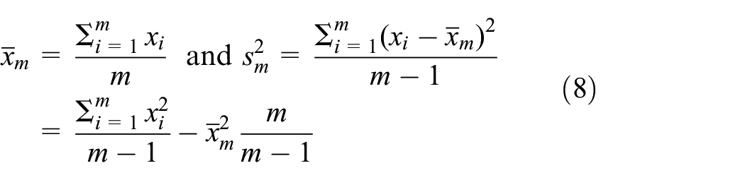
To define Hall’s SPRT, we follow Govindarajulu⁵ (Section 6.2.6). So, we take a pilot sample of size $m$ with $m$ ≥ 2, and compute the classic sample average and sample variance:

\begin{matrix} {\bar{x}}_{m} = \frac{Σ_{i = 1}^{m} x_{i}}{m} and s_{m}^{2} = \frac{Σ_{i = 1}^{m} {(x_{i} - {\bar{x}}_{m})}^{2}}{m - 1} \\ = \frac{Σ_{i = 1}^{m} x_{i}^{2}}{m - 1} - {\bar{x}}_{m}^{2} \frac{m}{m - 1} \end{matrix}

(8)

where the last equality simplifies the computation of $s_{m}^{2}$ . To compute ${\bar{x}}_{n}$ as $n$ increases, we use the update formula ${\bar{x}}_{n} = {\bar{x}}_{n - 1} (n - 1) / n + x_{n} / n$ with ${\bar{x}}_{0} = 0$ . To compute $s_{n}^{2}$ , we use the sum of squares about the average ${SS}_{n} = \sum_{i = 1}^{n} (x_{i} - {\bar{x}}_{n})^{2}$ , and the update formula ${SS}_{n} = {SS}_{n - 1} + (x_{n} - {\bar{x}}_{n - 1})^{2} (n - 1) / n$ with ${SS}_{0} = 0$ . These update formulas—plus references to alternative formulas—are presented in Kleijnen1992 (p.13). To improve the numerical accuracy of the variance estimate we might use the property that $x$ and $x - a$ with constant $a$ have the same variance; e.g., we may select $a = h_{1} / 2$ .

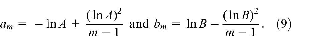
Hall’s SPRT uses the following boundaries assuming a pilot sample of size $m$ with $m \geq 2$ :

a_{m} = - \ln A + \frac{{(\ln A)}^{2}}{m - 1} and b_{m} = \ln B - \frac{{(\ln B)}^{2}}{m - 1} .

(9)

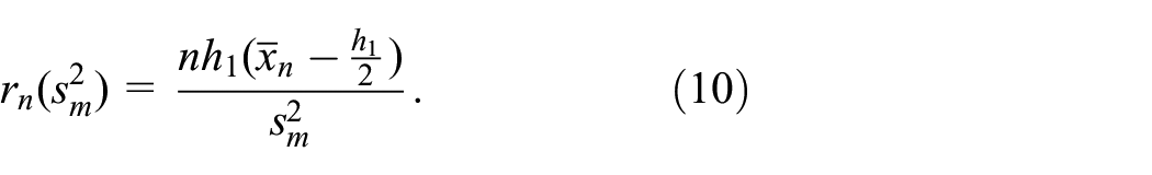
After $n$ observations with $n$ > $m$ , the test statistic is as follows:

r_{n} (s_{m}^{2}) = \frac{n h_{1} ({\bar{x}}_{n} - \frac{h_{1}}{2})}{s_{m}^{2}} .

(10)

Finally, this SPRT uses the following decision rule (where Equation (13) resembles Equation (7)):

Accept H_{0} if r_{n} (s_{m}^{2}) \leq b_{m},

(11)

accept H_{1} if r_{n} (s_{m}^{2}) \geq a_{m};

(12)

else, obtain x_{n + 1}, and compute r_{n + 1} (s_{m}^{2}) .

(13)

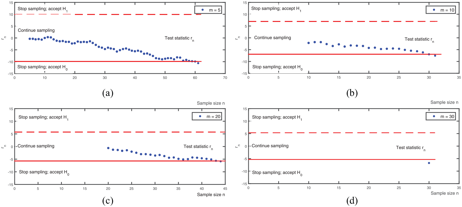
Hall’s SPRT has parallel boundaries (as Wald’s SPRT has), but as $m$ (pilot sample size) increases, these boundaries lie closer together so the continuation region gets smaller. For example, if $A = B = 0.01$ , then $a_{m} = 9.907$ if $m$ = 5, but $a_{m} = 5.038$ if $m$ = 50; likewise, $b_{m} = - 9.907$ if $m$ = 5 and $b_{m} = - 5.038$ if $m$ = 50. Finally, if $A = B$ , then Equation (9) implies $a_{m} = - b_{m}$ (analogous to Wald’s SPRT). Figure 2 displays results for $m =$ 5, 10, 20, and 30. Its four plots demonstrate that a smaller $m$ results in a larger $n_{f}$ (longer sample path); for example, Figure 2(a) (with $m$ = 5) shows the largest $n_{f}$ , and Figure 2(d) ( $m$ = 30) shows that the sample path becomes a single point. This property holds because a larger $m$ gives not only more accurate estimators ${\bar{x}}_{n}$ and $s_{m}^{2}$ in the test statistic defined in Equation (10), but also decreases the continuation region between the two boundaries so the sample path tends to hit one of the boundaries more quickly. However, if we select a “too big” value for $m$ , then no more observations are collected ( $n_{f}$ = $m$ ) and observations may be wasted. We conjecture that Hall’s SPRT requires a smaller $n_{f}$ than Wald’s SPRT does. To substantiate this conjecture, we shall conduct a MC experiment in Section 3.

Figure 2.

Example boundaries and sample path of Hall’s sequential probability ratio test for $x ~ N (0, 1)$ with different pilot sample size $m$ , when $h_{0}$ = 0 and $h_{1}$ = 0.5, $A = B = 0.01$ .

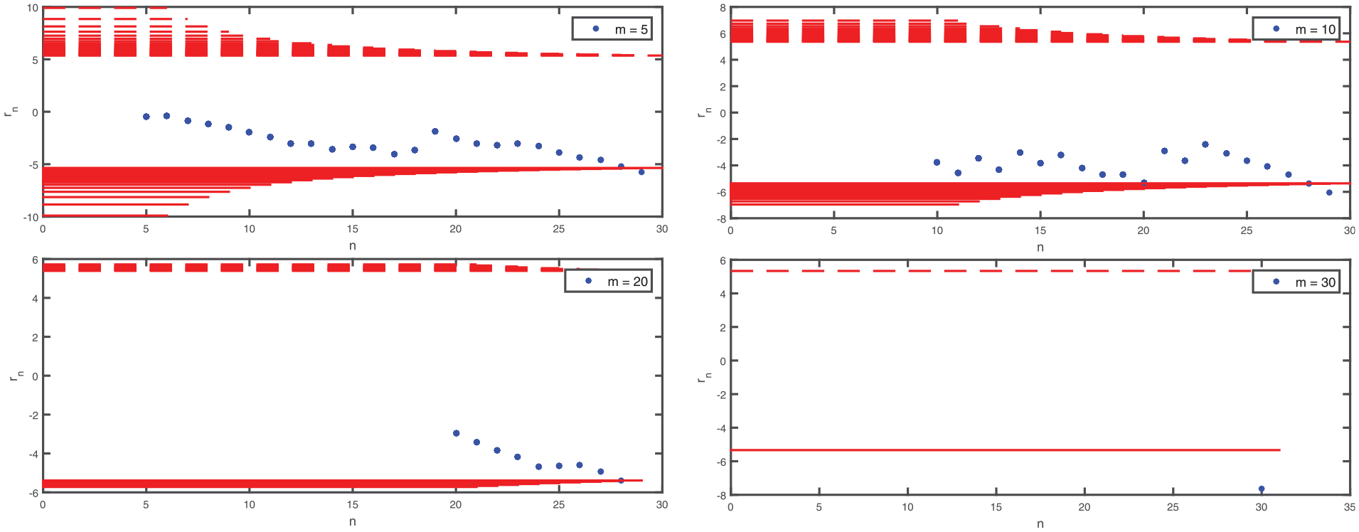
Hall’s⁶ modified SPRT replaces $s_{m}^{2}$ with $s_{n}^{2}$ ; that is, this modification updates the estimated variance after each additional observation, and replaces $m$ in Equation (8) through Equation (12) by $n$ . The modified boundaries $a_{n}$ and $b_{n}$ become closer to zero as $n$ increases (whereas $a_{m}$ and $b_{m}$ are constants—given $m$ ). Let us assume that—in the modified test statistic $r_{n} (s_{n}^{2})$ —the expected values of ${\bar{x}}_{n}$ and $s_{n}^{2}$ are constants (namely, $μ$ and $σ^{2}$ ), and let us ignore the nonlinearity of the transformation of ${\bar{x}}_{n}$ and $s_{n}^{2}$ implied by $r_{n} (s_{n}^{2})$ . Then $r_{n} (s_{n}^{2})$ tends to increase as $n$ increases and ${\bar{x}}_{n} > h_{1} / 2$ (where $h_{1} / 2$ is halfway between the hypothesized values of $μ$ in $H_{0}$ and $H_{1}$ , respectively), so the modified SPRT tends to accept $H_{1}$ . On the other hand, $r_{n} (s_{n}^{2})$ tends to decrease as $n$ increases and ${\bar{x}}_{n} < h_{1} / 2$ , so our SPRT tends to accept $H_{0}$ . We illustrate this SPRT in Figure 3, where the boundaries $a_{n}$ and $b_{n}$ are the horizontal lines that lie closer to zero as $n$ increases (see the red lines).

Figure 3.

Boundaries and sample path example for sequential probability ratio test with sequential estimator $s_{n}^{2}$ and pilot sample size $m$ , for $x ~ N (0, 1)$ with $h_{0}$ = 0, $h_{1} = 0.5$ , $A = B = 0.01$ . (Color online only.)

Comparing Figures 2 and 3 suggests that the modified SPRT gives results that are consistent with Hall’s original SPRT, for various $m$ . However, because this modified SPRT implies dynamic boundaries such that the continuation region tends to reduce as $n$ increases (but $s_{n}^{2}$ is random), this modified SPRT tends to require fewer observations than Hall’s original SPRT; for example, the plots show $n_{f}$ = 29 for the modified SPRT and $n_{f}$ = 61 for Hall’s original SPRT when $m_{0}$ = 5. To verify the results of this illustrative example, we use an extensive MC experiment in the next section.

3. Monte Carlo experiment #1: normal observations

In Section 3.1 we present details on the design of MC experiment #1: in Section 3.2 we detail the analysis of the results of this experiment. Because the design depends on the analysis that we plan to do, Section 3.1 also contains some analysis elements.

3.1. Experimental design

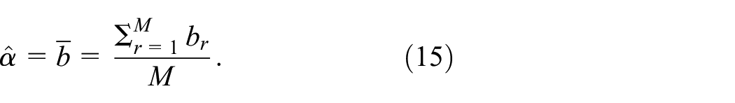
In this experiment we ensure that $x$ is indeed normally distributed. Whereas the preceding three figures displayed results for a single MC macroreplication, we now use $M$ = 1000 macroreplications; for example, to estimate $α$ , we use $M$ macroreplications with $M$ PRN-streams to sample from $N (h_{0}, σ)$ with the same $h_{0}$ and $σ$ . We select these $M$ streams such that the outcomes of the $M$ macroreplications are IID; that is, we use $M$ non-overlapping streams. To evaluate these outcomes, we use the following two performance measures (criteria): (i) $\hat{α}$ and $\hat{β}$ , which denote the estimators of $α$ and $β$ ( $\hat{α}$ is defined in Equation (15) below, and $\hat{β}$ is defined analogously); (ii) ${\bar{n}}_{f}$ , which denotes the final sample sizes averaged over the $M$ macroreplications. Our primary performance measures are $α$ and $β$ (defined in Equations (3) and (4), respectively). Obviously, our $\hat{α}$ is unbiased: $E (\hat{α}) = α$ . In Section 1 we have already observed that Wald⁴ (pp.132–133) and Hall⁶ (p.369) mention that their SPRTs are conservative, so we test the following:

H_{0}^{(α)} : E (\hat{α}) \leq A versus H_{1}^{(α)} : E (\hat{α}) > A,

(14)

where the superscript $(α)$ distinguishes these hypotheses from $H_{0}$ and $H_{1}$ in Equation (1). We use MATLAB to program our MC experiments; MATLAB includes Wald’s and Hall’s original SPRTs (see Govindarajulu⁵ (Section 6.2)).

To compute $\hat{α}$ , we sample $x$ from $N (μ, σ)$ . We select $μ$ = 0 because (without loss of generality) Hall’s SPRT assumes $h_{0}$ = 0 (see Section 2.2). Moreover, we—rather arbitrarily—select $σ$ = 1; higher values for $σ$ imply larger $n_{f}$ , which requires more computer time. Finally, we select $h_{1} = h_{0} + c σ$ where $h_{0}$ = 0 and $c$ is 0.5, 1, 2, and 3 so $h_{1}$ is 0.5, 1, 2, and 3; the higher $c$ is, the lower $n_{f}$ tends to be.

The $M$ macroreplications give $M$ IID Bernoulli outputs (say) $b_{r} (r = 1, \dots, M)$ where $b_{r}$ = 1 if macroreplication $r$ rejects $H_{0}$ and $b_{r}$ = 0 if it accepts $H_{0}$ . So, $P (b_{r} = 1) = α$ and $E (b_{r}) = α$ . These $b_{r}$ values give the fraction (percentage) of the $M$ macroreplications that rejects $H_{0}$ :

\hat{α} = \bar{b} = \frac{Σ_{r = 1}^{M} b_{r}}{M} .

(15)

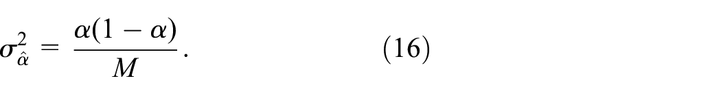
Because $b_{r}$ has a Bernoulli distribution, $\hat{α}$ has a binomial distribution with parameters $α$ and $M$ . This binomial distribution implies the following:

σ_{\hat{α}}^{2} = \frac{α (1 - α)}{M} .

(16)

To select a value for $M$ , we assume that the SPRTs are not conservative so $α$ = $A$ . Then, Equation (16) implies $σ_{\hat{α}} = [A (1 - A) / M]^{1 / 2}$ ; for example, if $A$ = 0.10, then $σ_{\hat{α}} = (0.09 / M)^{1 / 2}$ . The various SPRTs may give different values for $α$ and $σ_{\hat{α}}$ . For simplicity’s sake we select $M$ = 1000 for all combinations of $h_{1}$ , $A$ , $B$ , and SPRT. Please note that the formula for $σ_{\hat{α}}^{2}$ implies that it is easier to obtain a more “precise” estimate for $A$ closer to 1 than for $A$ closer to 0.5, where “precise” may be defined in an absolute sense ( $σ_{\hat{α}}^{2}$ ) or a relative sense ( $σ_{\hat{α}}^{2} / \hat{α}$ ).

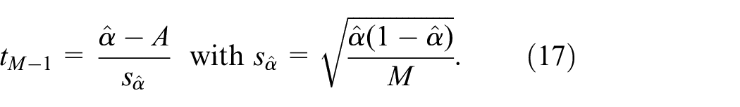
Our hypotheses in Equation (14) require a one-sided test. Using a Gaussian approximation of the binomial distribution of $\hat{α}$ , we obtain the following $t$ -statistic with $M - 1$ degrees of freedom:

t_{M - 1} = \frac{\hat{α} - A}{s_{\hat{α}}} with s_{\hat{α}} = \sqrt{\frac{\hat{α} (1 - \hat{α})}{M}} .

(17)

In general, the $t$ -statistic is known to be quite insensitive to non-normality. However, we do know that the Gaussian approximation is rougher as $\hat{α}$ is closer to its extreme value 0; that is, $\hat{α} < 0$ is impossible in the binomial distribution but not in the Gaussian distribution. Actually, if the SPRT results in $\hat{α}$ = 0 (so the denominator in Equation (17) becomes zero), then we need no refined mathematical statistics to reject $H_{1}^{(α)}$ . More generally, if $\hat{α} < A$ , then we do not reject $H_{0}^{(α)} : α \leq A$ . If $\hat{α} > A$ , then we reject $H_{0}^{(α)}$ only if $t_{M - 1} > t_{M - 1; 1 - p}$ , where $t_{M - 1; 1 - p}$ denotes the $1 - p$ quantile of the $t_{M - 1}$ distribution and $p$ denotes the type-I error rate of the test (this rate is usually denoted by $α$ , but we have already defined $α$ differently in Equation (3)). Because $M$ = 1000, we replace $t_{M - 1; 1 - p}$ with $z_{1 - p}$ where $z$ denotes the standard normal $N (0, 1)$ . The combination of this reasoning with Equation (17) gives the following decision rule:

Reject H_{0}^{(α)} if \hat{α} > A + z_{1 - p} s_{\hat{α}} .

(18)

Now we discuss the choice of a value for $p$ in $z_{1 - p}$ . We experiment not only with four values for $h_{1}$ (namely, 0.5, 1, 2, and 3; see above), but also with four values for $A$ and $B$ , respectively; namely, 0.01, 0.05, 0.10, and 0.20. Altogether we consider $4^{3}$ = 64 combinations of $(h_{1}, A, B)$ . For each combination we obtain a value for $t_{M - 1}$ . If we rejected $H_{0}^{(α)}$ if $t_{M - 1} > t_{M - 1; 1 - p}$ , then we would expect $p \times 64$ “false alarms” (type-I errors); for example, if $p$ = 0.10, then we expect 6.4 false alarms. We use a simple—but conservative—solution based on Bonferroni’s inequality; this solution does not exceed a prespecified experimentwise or familywise error rate (say) $F$ (this $F$ is the analogue of $A$ and $B$ ); “familywise” and “per comparison” error rates are discussed by Kleijnen¹ (p.98). So, in Equation (18) we replace $p$ with $F / 64$ . We select $F$ = 0.20; such a relatively high $F$ -value is usual, because such a value reduces the loss of power caused by the conservative Bonferroni inequality. $F$ = 0.20 implies that we use Equation (18) with $p = F / 64 = 0.20 / 64 = 0.003125$ , so $z_{1 - 0.003125} \approx 2.73$ . To improve the precision of our comparisons—across various SPRTs, 64 combinations $(h_{1}, A, B)$ , and various distributions of $x$ —we use CRNs, as we explain in great detail in Appendix 3.

3.2. Analysis of the experiment

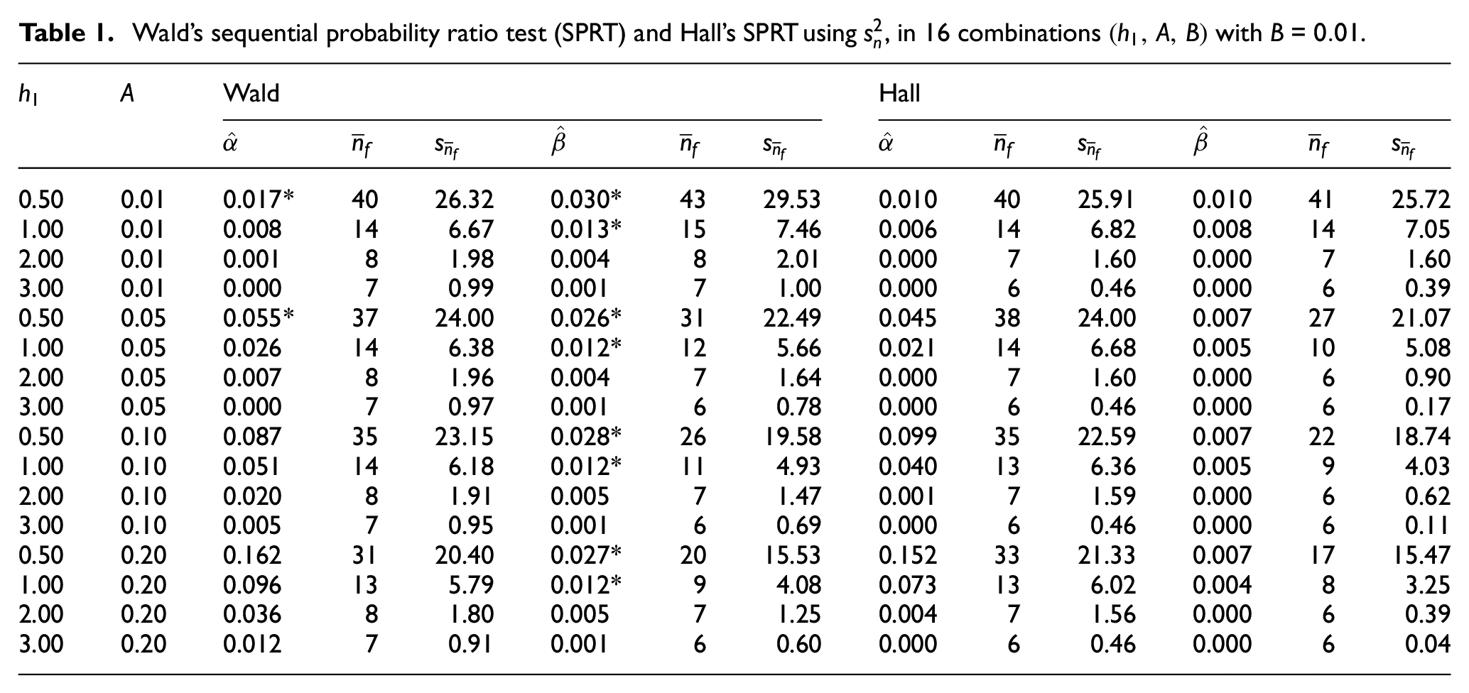
Table 1 displays results for Wald’s SPRT and Hall’s SPRTs—both modified so they use $s_{n}^{2}$ (we do not display results for the SPRTs that use $s_{m}^{2}$ , because these results are inferior)—and only 16 of the 64 combinations of $(h_{1}, A, B)$ —namely, the combinations in which $B$ is 0.01; the remaining 48 combinations in which $B$ is 0.05, 0.10, or 0.20 give similar results, so we display those results in Appendix 4 (actually, we shall see that the effect of $B$ on $\hat{β}$ resembles the effect of $A$ on $\hat{α}$ , and Table 1 does show all four values for $A$ ). Because of Equation (18), we reject $H_{0}^{(α)}$ if $\hat{α} > A + 2.73 s_{\hat{α}}$ with $s_{\hat{α}} = [\hat{α} (1 - \hat{α}) / M]^{1 / 2}$ ; to denote significantly high values in Table 1, we use an asterisk (*). Before we further comment on $\hat{α}$ , we now discuss $\hat{β}$ (which has its own ${\bar{n}}_{f}$ and $s_{{\bar{n}}_{f}}$ ; see the columns after $\hat{β}$ in Table 1).

Table 1.

Wald’s sequential probability ratio test (SPRT) and Hall’s SPRT using $s_{n}^{2}$ , in 16 combinations $(h_{1}, A, B)$ with $B$ = $0.01$ .

$h_{1}$	$A$	Wald						Hall
		$\hat{α}$	${\bar{n}}_{f}$	$s_{{\bar{n}}_{f}}$	$\hat{β}$	${\bar{n}}_{f}$	$s_{{\bar{n}}_{f}}$	$\hat{α}$	${\bar{n}}_{f}$	$s_{{\bar{n}}_{f}}$	$\hat{β}$	${\bar{n}}_{f}$	$s_{{\bar{n}}_{f}}$
0.50	0.01	0.017*	40	26.32	0.030*	43	29.53	0.010	40	25.91	0.010	41	25.72
1.00	0.01	0.008	14	6.67	0.013*	15	7.46	0.006	14	6.82	0.008	14	7.05
2.00	0.01	0.001	8	1.98	0.004	8	2.01	0.000	7	1.60	0.000	7	1.60
3.00	0.01	0.000	7	0.99	0.001	7	1.00	0.000	6	0.46	0.000	6	0.39
0.50	0.05	0.055*	37	24.00	0.026*	31	22.49	0.045	38	24.00	0.007	27	21.07
1.00	0.05	0.026	14	6.38	0.012*	12	5.66	0.021	14	6.68	0.005	10	5.08
2.00	0.05	0.007	8	1.96	0.004	7	1.64	0.000	7	1.60	0.000	6	0.90
3.00	0.05	0.000	7	0.97	0.001	6	0.78	0.000	6	0.46	0.000	6	0.17
0.50	0.10	0.087	35	23.15	0.028*	26	19.58	0.099	35	22.59	0.007	22	18.74
1.00	0.10	0.051	14	6.18	0.012*	11	4.93	0.040	13	6.36	0.005	9	4.03
2.00	0.10	0.020	8	1.91	0.005	7	1.47	0.001	7	1.59	0.000	6	0.62
3.00	0.10	0.005	7	0.95	0.001	6	0.69	0.000	6	0.46	0.000	6	0.11
0.50	0.20	0.162	31	20.40	0.027*	20	15.53	0.152	33	21.33	0.007	17	15.47
1.00	0.20	0.096	13	5.79	0.012*	9	4.08	0.073	13	6.02	0.004	8	3.25
2.00	0.20	0.036	8	1.80	0.005	7	1.25	0.004	7	1.56	0.000	6	0.39
3.00	0.20	0.012	7	0.91	0.001	6	0.60	0.000	6	0.46	0.000	6	0.04

Given the definition of $β$ in Equation (4), we compute $\hat{β}$ through sampling from $N (h_{1}, σ)$ (instead of $N (h_{0}, σ)$ , which we used for $\hat{α}$ ). The CRN implies that—instead of sampling $x_{i} ~ N (0, 1)$ $(i = 1, \dots, n)$ —we sample $y_{i} = x_{i} + (h_{1} - h_{0})$ , so $\bar{y} = \bar{x} + (h_{1} - h_{0})$ and $s_{y}^{2} = s_{x}^{2} = s^{2}$ . Because $h_{0}$ = 0 in Equation (10), the test statistic $r_{n} (s_{n}^{2})$ increases with ${nh}_{1}^{2} / s_{n}^{2}$ . Hence, the new $r_{n} (s_{m}^{2})$ is always higher than the old $r_{n} (s_{m}^{2})$ computed under $H_{0}$ . Our test for $\hat{β}$ is the analogue of the test for $\hat{α}$ in Equation (18). Because the SPRTs treat $H_{0}$ and $H_{1}$ similarly, we conjecture that $\hat{α}$ and $\hat{β}$ exhibit similar behavior. To test this conjecture, we use a second-degree polynomial regression model, as we shall explain below (in the paragraph containing Equation (19)).

Combining Table 1 and the table in Appendix 4 shows that either $\hat{α}$ = 0.000 or $\hat{β}$ = 0.000 in 92 of the 128 combinations (namely, 64 combinations for $\hat{α}$ and 64 combinations for $\hat{β}$ ). This value of 0.000 means that none of the $M$ = 1000 macroreplications cross the “wrong” boundary. Focusing on these 92 combinations, we try to discover whether specific values of $h_{1}$ , $A$ , or $B$ —or combinations of these values—give these extremely low $\hat{α}$ or $\hat{β}$ . We conclude that all combinations with $\hat{α}$ = 0.000 or $\hat{β}$ = 0.000 have a very large $h_{1}$ and a very small ${\bar{n}}_{f}$ ; that is, combinations with $h_{1} >> h_{0}$ imply that the SPRTs require only a small sample to make the correct decision.

Furthermore, several combinations in Table 1 and the table in Appendix 4 give a significantly high $\hat{α}$ or $\hat{β}$ for Wald’s modified SPRT, whereas Hall’s modified SPRT is conservative. This conclusion seems reasonable: after all, Hall’s SPRT is derived for the special case of a normal distribution with an unknown variance.

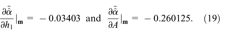
Now we test whether indeed $\hat{α}$ and $\hat{β}$ show similar behavior. For each of the two SPRTs, we first fit a second-degree polynomial with the explained regression variables $\tilde{\hat{α}}$ (where the tilde denotes a regression estimate; $\hat{α}$ denotes the estimate resulting from the MC experiment) and $\tilde{\hat{β}}$ , respectively; the three explanatory variables are $h_{1}$ , $A$ , and $B$ . We present the (tedious) regression analysis in Appendix 5. This analysis uses the least squares (LS) criterion to fit these two polynomials to the $4^{3}$ = 64 combinations of $(A, B, h_{1})$ . This fitting gives estimated coefficients for these polynomials and their standard deviations (or standard errors). So, we can test whether these estimated coefficients (or parameters) significantly differ from zero. We eliminate non-significant effects from the full polynomials, which gives the reduced polynomials. Finally, we use these reduced (simplified, parsimonious) polynomials to check whether the marginal effects of the explanatory variables are “understandable”; that is, do they have the correct signs? Therefore, we compute the marginal effects implied by the reduced polynomials, at the midpoint (or center) of our experimental area, $m = ({\bar{h}}_{1}, \bar{A}, \bar{B})^{'} = (1.625, 0.09, 0.09)^{'}$ :

\frac{\partial \tilde{\hat{α}}}{\partial h_{1}} |_{m} = - 0.03403 and \frac{\partial \tilde{\hat{α}}}{\partial A} |_{m} = - 0.260125 .

(19)

So, a higher $h_{1}$ gives a lower $\tilde{\hat{α}}$ , which makes sense because the SPRT can easily make the correct selection when the two hypothesized values are far apart. A higher $A$ gives a lower $\tilde{\hat{α}}$ , which may be explained by the negative interaction between $h_{1}$ and $A$ in the reduced polynomial (again see Appendix 5).

Next we repeat our analysis for $\hat{β}$ . The results in Appendix 5 suggest that $\tilde{\hat{α}}$ and $\tilde{\hat{β}}$ indeed respond in a similar way to $h_{1}$ , $A$ , and $B$ ; for example, the effect of $A$ on $\tilde{\hat{α}}$ is $0.694$ , the effect of $B$ on $\tilde{\hat{β}}$ is $0.767$ , and these two estimates do not differ significantly.

Finally, we examine ${\bar{n}}_{f}$ (our secondary performance measure; see the text above Equation (14)). Table 1 clearly demonstrated that the modification accounting for unknown $σ$ in Wald’s SPRT for $N (μ, σ)$ gives significantly high $\tilde{\hat{α}}$ or $\hat{β}$ for many combinations $(h_{1}, A, B)$ . We therefore do not consider ${\bar{n}}_{f}$ and its standard deviation $s_{{\bar{n}}_{f}}$ for this modified SPRT; that is, we limit our regression analysis of ${\bar{n}}_{f}$ to the modification of Hall’s SPRT. If more than one SPRT gave $α \leq A$ and $β \leq B$ and we are risk neutral instead of risk averse or risk seeking, then we would prefer the SPRT with the smallest $μ_{n_{f}}$ . To analyze ${\bar{n}}_{f}$ , we apply the same type of regression analysis as we applied for $\tilde{\hat{α}}$ and $\hat{\tilde{β}}$ (see the last part of Appendix 5). The resulting reduced polynomial gives the following.

\frac{\partial {\tilde{\bar{n}}}_{f} (α)}{\partial h_{1}} |_{m} = - 7.7396 and \frac{\partial {\tilde{\bar{n}}}_{f} (α)}{\partial B} |_{m} = - 32.8596 .

So, a higher $h_{1}$ or $B$ decreases ${\tilde{\bar{n}}}_{f} (α)$ , because these factors have important negative first-order effects (namely, $- 30.062$ and $- 89.512$ ; again see Appendix 5).

We conclude the following:

Wald’s modified SPRT gives significantly high $\hat{α}$ or $\hat{β}$ for many $(h_{1}, A, B)$ combinations, whereas Hall’s modified SPRT is conservative;

$\tilde{\hat{α}}$ and $\tilde{\hat{β}}$ respond to $h_{1}$ , $A$ , and $B$ in similar ways;

if $h_{1}$ , $A$ , or $B$ increases, then ${\tilde{\bar{n}}}_{f}$ of Hall’s modified SPRT decreases.

4. Experiment #2: non-normal observations

In MC experiment # 2 we sample observations $x$ that are not normally distributed, so that we can investigate whether the SPRTs are robust; that is, are the SPRTs “quite” insensitive to non-normality? There are infinitely many types of non-normal distributions, but we limit our experiment to the following three distribution types: (i) lognormal, (ii) gamma, and (iii) exponential. Now we detail our design and analysis for the lognormal distribution.

By definition, $y$ has a lognormal distribution with shape parameter $σ > 0$ and scale parameter $\exp (μ) > 0$ —denoted as $y ~ LN (μ, σ)$ —if $\ln y ~ N (μ, σ)$ . The following relations are well known: $μ_{y} = \exp (μ + σ^{2} / 2)$ and $σ_{y}^{2} = \exp (2 μ + σ^{2}) (\exp σ^{2} - 1)$ . Lognormal distributions may have various shapes; for example, if $σ$ = 1, then these distributions are very skew so they are very non-normal. Samples from $LN (μ, σ)$ cannot be negative. For more details we refer to Law² (pp.294–295).

In our MC experiment we use $LN (μ, σ)$ with $μ$ = 0 and $σ$ = 1; consequently, $μ_{y} = \exp (1 / 2) \approx 1.65$ and $σ_{y}^{2} = \exp (1) (\exp 1 - 1) \approx 4.7$ . In Section 2.2 we saw that Hall⁶ assumes $x ~ N (μ, σ)$ with $μ$ = 0 in $H_{0}$ , so we apply the transformation $x = y - μ_{y}$ with $μ_{y} \approx 1.65$ so $μ_{x}$ = 0 (so we shift the lognormal to the left). Furthermore, the combination $μ$ = 0 and $σ$ = 1 implies that our shifted lognormal distribution with mean 0 has variance $e (e - 1) \approx 4.7$ or standard deviation 2.17 approximately. Below Equation (14) we selected $h_{1} = h_{0} + c σ$ with $h_{0}$ = 0, $σ$ = 1, and $c$ is 0.5, 1, 2, and 3; so, $h_{1}$ was 0.5, 1, 2, and 3. Now we select $h_{0}$ = 0 and $h_{1} = c σ$ with $σ$ = 2.17 so $h_{1}$ is 1.09, 2.17, 4.34, and 6.51. Whatever values we select for $h_{0}$ and $h_{1}$ , the SPRT should guarantee $α \leq A$ ; we conjecture that a higher $| h_{0} - h_{1} |$ decreases $μ_{n_{f}}$ (expected value of $n_{f}$ ), because it becomes easier for the SPRT to select $H_{0}$ or $H_{1}$ .

Furthermore, we compare $\tilde{\hat{α}}$ for normal and lognormal distributions. To increase the precision of this comparison, we again use CRNs (in MC experiment #1, we used CRNs to compare combinations of $h_{1}$ , $A$ , $B$ , and SPRT). Now it is again easy to apply CRNs: when sampling from $LN (μ, σ)$ , the PRN-streams remain “synchronized” with sampling from $N (μ, σ)$ (for details on “synchronization” we refer to Law² (pp.592–598)): to sample from $y ~ LN (μ, σ)$ , we sample $z ~ N (μ, σ)$ and compute $y = \exp z$ and $x = y - μ_{y}$ ; also see Appendix 6, which covers lognormal samples and normal samples while applying CRNs.

To design experiment #2, we use the results of our analysis of experiment #1. This analysis showed that a second-degree polynomial in the factors $h_{1}$ , $A$ , and $B$ is an adequate model of the reaction of $\tilde{\hat{α}}$ or $\hat{β}$ to these three factors. To fit such a polynomial, we now use a modified CCD. Classic CCDs are discussed by Kleijnen¹ (pp.63–66). Compared with the $4^{3}$ design in MC experiment #1, a CCD saves computer time because it has fewer factor combinations (this $4^{3}$ design is detailed in Table 1 and Appendix 4). We modify the classic CCD such that it has only 14 combinations, which are specified in the first three columns of Table 2; we detail the classic CCD and our modified CCD in Appendix 7. Our modified CCD in MC experiment \#1 is a proper subset of the $4^{3}$ design in MC experiment \#1; e.g., combination 6 in Table 1 also occurs in Table 2 in the main text (because it combines the low axial point $B = 0.01$ with the low intermediate values $h_{1} = 2.17$ and $A = 0.05$ in the $2^{2}$ design; again see Appendix 7), whereas combination 1 in Table 1 does not occur in Table 2 in the main text (because it combines the low axial points for all three factors; again see Appendix 7). The 14 combinations of our modified CCD are well spread over the experimental area, but they are sparser than the $4^{3}$ combinations and do not form a so-called balanced design.

Table 2.

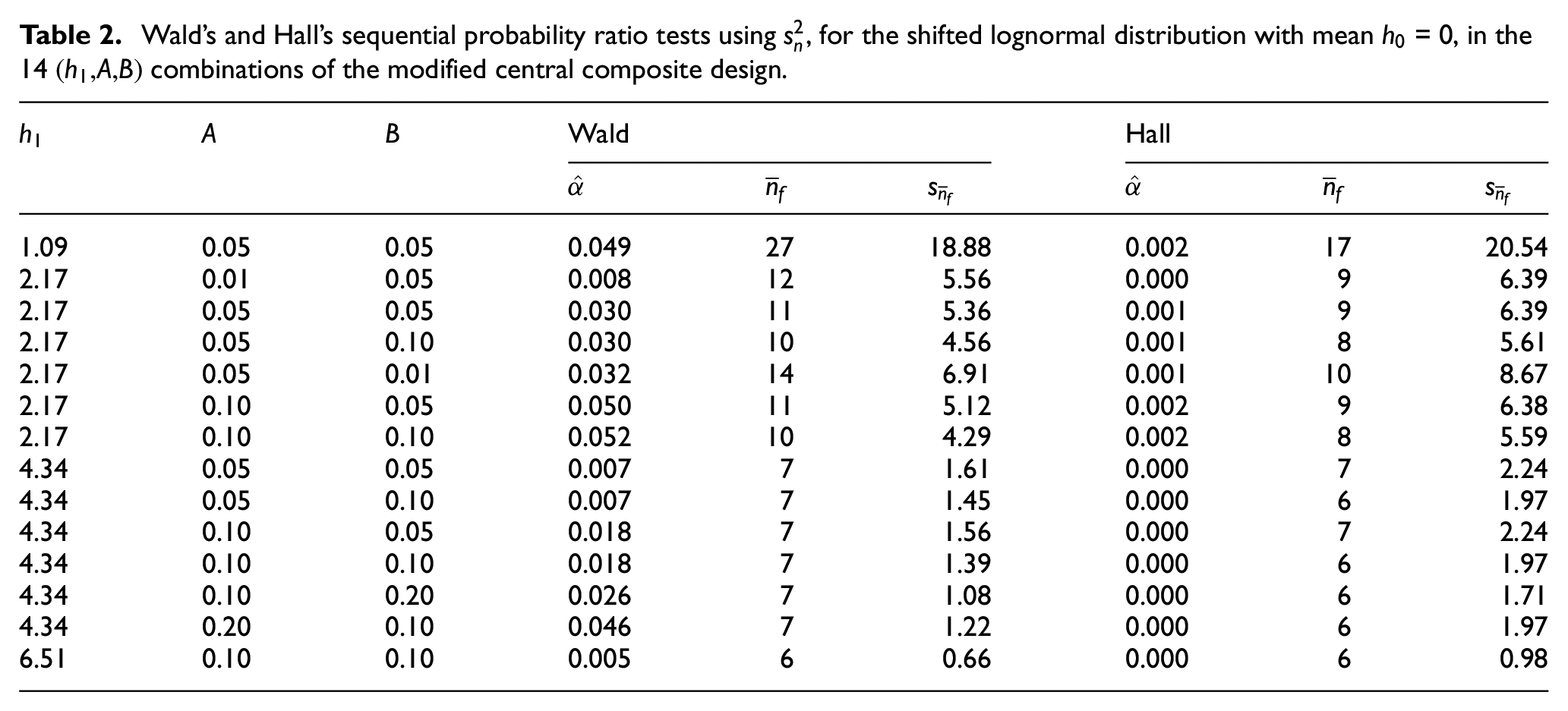
Wald’s and Hall’s sequential probability ratio tests using $s_{n}^{2}$ , for the shifted lognormal distribution with mean $h_{0}$ = 0, in the 14 $(h_{1}, A, B)$ combinations of the modified central composite design.

$h_{1}$	$A$	$B$	Wald			Hall
			$\hat{α}$	${\bar{n}}_{f}$	$s_{{\bar{n}}_{f}}$	$\hat{α}$	${\bar{n}}_{f}$	$s_{{\bar{n}}_{f}}$
1.09	0.05	0.05	0.049	27	18.88	0.002	17	20.54
2.17	0.01	0.05	0.008	12	5.56	0.000	9	6.39
2.17	0.05	0.05	0.030	11	5.36	0.001	9	6.39
2.17	0.05	0.10	0.030	10	4.56	0.001	8	5.61
2.17	0.05	0.01	0.032	14	6.91	0.001	10	8.67
2.17	0.10	0.05	0.050	11	5.12	0.002	9	6.38
2.17	0.10	0.10	0.052	10	4.29	0.002	8	5.59
4.34	0.05	0.05	0.007	7	1.61	0.000	7	2.24
4.34	0.05	0.10	0.007	7	1.45	0.000	6	1.97
4.34	0.10	0.05	0.018	7	1.56	0.000	7	2.24
4.34	0.10	0.10	0.018	7	1.39	0.000	6	1.97
4.34	0.10	0.20	0.026	7	1.08	0.000	6	1.71
4.34	0.20	0.10	0.046	7	1.22	0.000	6	1.97
6.51	0.10	0.10	0.005	6	0.66	0.000	6	0.98

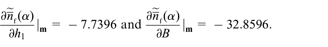
Our analysis of experiment #1 showed that $\tilde{\hat{α}}$ and $\hat{β}$ give similar results, so in experiment #2 we estimate only $\hat{α}$ (not $\hat{β}$ ); that is, we sample only from a distribution with mean $h_{0}$ = 0 (not $h_{1}$ ). We again use $M$ = 1000 macroreplications. Table 2 shows that (i) both SPRTs give $\hat{α} < A$ in all combinations, and (ii) Wald’s modified SPRT (using $s_{n}^{2}$ ) often requires a higher ${\bar{n}}_{f}$ . Hall’s modified SPRT (using $s_{n}^{2}$ instead of $s_{m}^{2}$ ) gives $\hat{α}$ = 0.000 if $h_{1}$ ≥ 4.34 and if $A$ = 0.01. Cursory inspection of this table suggests that $\hat{α}$ does respond to $A$ ; to quantify this response function we again apply regression analysis (see Appendix 8). The design and analysis of our experiments with the other two non-normal distributions (namely, gamma and exponential) are detailed in Appendixes 9 and 10. In Appendix 11 we investigate whether a normalizing transformation of $x$ may reduce ${\bar{n}}_{f}$ . We focus on the simplest normalizing transformation; namely, the logarithmic transformation. Our MC experiment \#3 shows that this transformation does not decrease ${\bar{n}}_{f}$ ; neither does it decrease $\hat{α}$ .

Altogether, experiment #2 gives the following results, where “Wald” and “Hall” mean Wald’s and Hall’s modified SPRTs using $s_{n}^{2}$ , respectively.

Lognormal: (i) both Wald and Hall give $\hat{α} < A$ in all 14 combinations of ( $h_{1}$ , $A$ , $B$ ), and (ii) Wald often requires a higher ${\bar{n}}_{f}$ . (See Table 2.)

Gamma: (i) both Wald and Hall give $\hat{α} < A$ in all 14 combinations, and (ii) Wald requires a smaller ${\bar{n}}_{f}$ than Hall does. (See Appendix 9.)

Exponential: (i) both Wald and Hall give $\hat{α} < A$ in all 14 combinations, (ii) Wald requires a smaller ${\bar{n}}_{f}$ than Hall does, and (iii) Wald’s non-modified SPRT for exponential distributions gives $\hat{α} < A$ in all 14 combinations and requires a smaller ${\bar{n}}_{f}$ than Wald’s modified SPRT in 13 of the 14 combinations. (See Appendix 10.)

We conclude that the SPRTs give $\hat{α} < A$ in all 14 combinations of ( $h_{1}$ , $A$ , $B$ )—so the SPRTs are “conservative”—even if the distribution is non-normal—so the SPRTs are “robust.” Our explanation is that Hall’s test statistic $r_{n} (s_{n}^{2})$ (defined in Equation (10)) resembles the classic $t$ -statistic, which is quite insensitive to non-normality. Wald’s test statistic $S$ (see Equation (2)) is a sum of random variables, so the central limit theorem (CLT) applies. Which SPRT requires a smaller ${\bar{n}}_{f}$ is not so clear; if we assume an exponential PDF, then Wald’s non-modified SPRT requires a smaller ${\bar{n}}_{f}$ . However, our experiment #1 with a normal PDF showed that Wald’s modified SPRT gives significantly high $\hat{α}$ for many combinations (whereas Hall’s modified SPRT is conservative)—which seems to contradict our conclusions based on experiment #2. Altogether, we recommend Hall’s modified SPRT—pending further research.

5. Conclusions and future research

For the testing of two hypothesized values of a mean output, we reviewed Wald’s⁴ and Hall’s⁶ original SPRTs, and two simple modifications. For these SPRTs we used plots to illustrate both the boundaries—which define their continuation areas—and possible sample paths of their test statistics.

We designed our MC experiment #1 such that the output is guaranteed to be normally distributed. This experiment showed that Wald’s SPRT modified for unknown output variance may give significantly high $\hat{α}$ (estimated type-I error rate) or $\hat{β}$ (estimated type-II error rate) for some factor combinations in the experiment. However, if we modify Hall’s SPRT to get a sequential estimator of the output variance, then the resulting SPRT is conservative; that is, this SPRT gives significantly low $\hat{α}$ or $\hat{β}$ . Furthermore, our regression analysis of MC experiment #1 showed that $\hat{α}$ and $\hat{β}$ exhibit similar reactions to $h_{1} - h_{0}$ (difference between the hypothesized value $h_{1}$ in hypothesis $H_{1}$ and $h_{0}$ in $H_{0}$ ), $A$ (prespecified nominal $α$ ), and $B$ (nominal $β$ ). Finally, $n_{f}$ (final sample size of the SPRT) decreases for increasing $h_{1} - h_{0}$ , $A$ , or $B$ .

Our MC experiment #2 used three types of non-normal distributions; namely, lognormal, gamma, and exponential distributions. This experiment showed that the SPRTs are quite robust; that is, $\hat{α}$ and $\hat{β}$ remain below $A$ and $B$ . Our explanation was that Hall’s test statistic resembles the classic $t$ -statistic; Wald’s test statistic uses a sum of IID variables so the CLT applies.

We hope that in the near future other researchers will repeat and extend our research—possibly applying our methodology for the design and analysis of MC experiments with SPRTs. Finally, we hope to investigate SPRTs for more than a single mean output.

Supplemental Material

sj-pdf-1-sim-10.1177_0037549720954916 – Supplemental material for Sequential probability ratio tests: conservative and robust

Supplemental material, sj-pdf-1-sim-10.1177_0037549720954916 for Sequential probability ratio tests: conservative and robust by Jack PC Kleijnen and Wen Shi in SIMULATION

Footnotes

Acknowledgements

We thank Ruud Brekelmans (Tilburg University) for helping us solve the problem of avoiding overlap among PRN-streams when applying CRNs. We thank three anonymous referees for their comments that helped us to clarify some issues and improve our presentation.

Funding

The work of Wen Shi was partially supported by the National Natural Sciences Foundation of China (Grant Nos. 71971219, 71790615, and 71991463).

ORCID iD

Wen Shi

Author biographies

Jack PC Kleijnen is Emeritus Professor of “Simulation and Information Systems” at Tilburg University (TiU), where he is still an active member of both the Department of Management and the Operations Research Group of the Center for Economic Research (CentER) in the Tilburg School of Economics and Management (TiSEM). He is also an active author and reviewer for many international journals. His email address is kleijnen@tilburguniversity.edu.

Wen Shi is a Professor in Business School at Central South University. He holds a PhD in management science and engineering from Huazhong University of Science and Technology. His research focuses on simulation modeling, simulation experiment design and analysis, and supply chain management. His email address is shi3wen@163.com.

References

Kleijnen

JPC

. Design and analysis of simulation experiments. 2nd ed. New York: Springer US, 2015.

Law

. Simulation modeling and analysis. 6th ed. Boston, MA: McGraw-Hill, 2015.

Kleijnen

JPC

. Statistical techniques in simulation: Part II. New York: Dekker, 1975.

Wald

. Sequential tests of statistical hypotheses. Ann Math Stat 1945; 16: 117–186.

Govindarajulu

. Sequential statistics. Singapore: World Scientific, 2014.

Hall

. Some sequential analogs of Stein’s two-stage test. Biometrika 1962; 49: 367–378.

Zeigler

Praehofer

Kim

. Theory of modeling and simulation: Integrating discrete event and continuous complex dynamic systems. San Diego, CA: Academic Press, 2000.

Supplementary Material

Please find the following supplemental material available below.

For Open Access articles published under a Creative Commons License, all supplemental material carries the same license as the article it is associated with.

For non-Open Access articles published, all supplemental material carries a non-exclusive license, and permission requests for re-use of supplemental material or any part of supplemental material shall be sent directly to the copyright owner as specified in the copyright notice associated with the article.

0.00 MB

0.15 MB