Direct simulation of thermally and mechanically coupled particle-laden flow

Abstract

This work describes a unique technique to simulate continuously and directly coupled fluid flow and moving particles including both mechanical and thermal interactions between the flow, particles, and flow paths. The particles/flow paths are discretized within a computational fluid dynamics flow domain so that the local flow and temperature field conditions surrounding each particle or other solid body are known along with the local temperature distribution within the particle and other solids. Contact conduction between solid bodies including contact resistance, conjugate heat transfer at the fluid–solid interfaces, and even radiation exchanges between solid surfaces and between solid surfaces and the fluid are incorporated in the thermal interactions and a soft collision model simulates the solid body mechanical contact. The ability to capture these local flow and thermal effects removes reliance on correlations for fluid forces and for heat transfer coefficients/exchange and removes restrictions on the flow regime and particle size and volume fraction considered. Larger particle sizes and higher particle concentration conditions can be studied with local effects captured. The method was tested for a range of particle thermal and mechanical properties, driving pressures, and for limited radiation parameters. The results reveal important information about the basic thermal and flow phenomena that cannot be obtained in standard modeling methods and demonstrate the utility of the modeling method. The technique can be applied to examine phenomena dependent on local thermal conditions such as chemical reactions, material property variation, agglomerate formation, and phase change. The methods can also be used as a basis for machine learning algorithm development for flows with large particle counts so that more detailed phenomena can be considered compared to those provided by standard techniques with reduced computational costs compared to those with fully resolved particles in the flow.

Keywords

Particle flow thermal interaction mechanical interaction computational fluid dynamics heat transfer

1. Introduction

Particle-laden compressible flow is fundamental to many processes, and in many cases, the phenomena of interest in these flows are dependent on the local temperature or flow conditions at the particle–fluid interfaces. To simulate such events including chemical reactions or phase changes at these interfaces, the localized, time-varying state of the particles and the flow must be available. Furthermore, while coupling of the discrete element method (DEM) and computational fluid dynamics (CFD) has been used to capture interacting particles within a fluid flow when the particle volumes are larger and when particle–particle interactions are frequent, these methods cannot be used to obtain the localized flow and particle state since the particles are not directly discretized within the computational domain. Instead, correlation equations for the coefficient of drag are used to formulate the fluid induced forces, limiting the particle arrangements and flow conditions that can be studied. Heat transfer coefficients are used to estimate the heat exchange between the particles and the flow, restricting conditions to those for which coefficients have been developed. Heat conduction through the particles, or other solids, particularly upon solid–solid contact, if considered, is commonly treated using a lumped parameter technique. Often, localized temperatures at a particle–fluid interface may be critical to determining when a chemical reaction begins and how burning or phase change varies along the surface of a particle. Because the localized variations in the conditions cannot be obtained from standard particle flow techniques, the analysis of such events cannot be undertaken.

A series of modeling methods has been developed to fill the gap in the modeling capabilities to provide means to study particle-laden flow phenomena that require localized particle and flow information for analysis of a particular effect and for conditions with large particles, high particle concentration, or frequent particle interaction, focusing on compressible flow conditions.^1–6 Particle motion in compressible flow involves high temperature and velocity gradients at the flow–particle interfaces. By resolving the actual particles in the fluid flow through direct particle computational discretization, well-defined boundary conditions and turbulence models can be applied. Velocity and temperature gradients at the interface as well as local temperatures, pressures, or even species concentrations anywhere in the system can be obtained. Typical DEM-CFD coupling cannot provide such information including the local gradients at the particle–flow interfaces, the local flow conditions near the interface, the temperatures within the particle, and the variations in the flow and thermal conditions along the surface of the particles. In addition, with closely positioned, large particles, correlations needed to model the fluid–particle interactions may not exist and may not be valid for when the flow and thermal conditions may vary significantly along the particle surface. Previous work by the author has shown that mechanical interactions between particles moving within a high speed flow can be incorporated into direct particle motion modeling methods, removing the need for correlations for drag and removing restrictions on the particle arrangements and sizes that can be studied. Previous work by the author also demonstrated that frictional, rolling, and adhesion effects can be included in the particle–particle interaction effects while directly accounting for the moving particles in the flow.^1–4 These phenomena are all local and can produce variations in the temperature and flow fields near the particle surfaces. Next, means to include contact conduction effects along with convection and radiation were developed and tested for fixed particles,^5,6 again allowing for the local rather than lumped temperature field development due to these heat transfer modes. This current work reports on the advancement of the modeling method to include the combination of the mechanical and thermal interactions between particles and the flow and particles and other particles, with radiation exchange between surfaces in high speed compressible flow with moving particles in the flow instead of fixed particles. The objective of this work is to describe the new technique for simulating the detailed, local particle and flow conditions within particle-laden flow, and to demonstrate the new capabilities and advantages offered over standard methods.

For modeling the mechanical interactions of the particles under conditions where the particle–particle interactions are significant, one of the most widely used methods is the discrete element model (DEM)-based model which typically combines Lagrangian particle tracking with an Eulerian flow–particle model. The particles are treated as a secondary “fluid” with particle interactions with the flow requiring correlations for drag and “viscosity.” Thermal interactions between the particles and the flow require heat transfer coefficient correlations. Mechanical interactions between two objects are captured through non-linear springs and dampers with the magnitude of these forces varying with the amount of “overlap” of the particles or other objects from their undeformed shape.⁷ Multiple, simultaneously contacting particles can be readily handled and various material models can be implemented as described in Di Renzo and Di Maio.⁸ Thermal interactions between particles may or may not be included, but generally involve a simplified, bulk temperature-based model for the thermal conditions in the particles. The localized flow effects as the particles interact and move closer and further from one another are lost, the localized temperature fields near the particle–fluid interface and through the particles, and other data like species concentrations are not captured with this method. New locations of the particles are determined based on the fluid and interaction forces, but this information is only used to formulate a new particle volume fraction distribution as individual particles are not included in the flow domain. The Eulerian two-fluid model is then used to solve for the thermal and flow conditions in the system. A range of systems can be studied in this manner with the work of Tsuji et al.,⁹ an early application of this method, the work of Chen et al.¹⁰ used to predict the particle flow in pulmonary airways, and the work of Grof et al.¹¹ used a modification to examine agglomerates. Lacking information about the near particle–fluid interfaces including flow, temperature, and species mass fractions and their gradients, events driven by these conditions cannot be studied nor can conditions for which correlations for drag or the heat transfer coefficient are not available or when their use may not be valid.

Methods to incorporate thermal interactions between particles in a DEM-Eulerian type model is an area of active research, first with simpler models. Vargas and McCarthy¹² apply a lumped capacitance, uniform temperature model to examine the temperatures as two solid particles contact. To study the thermal conditions in a particle bed, Liu and Li¹³ use a uniform, lumped particle temperature model to estimate the conduction heat exchange at contact, a correlation for the heat transfer coefficient for convection, and gray body radiation exchange between the particle surface at bulk temperature and the container surface at its bulk temperature. Yang et al.¹⁴ estimate convective heat transfer from a particle surface through a correlation and use analytical methods to model contacting particles with each particle at a uniform temperature. Cheng and Zhang,¹⁵ in a study of the combustion process of propellant grains, use a quasi-steady, semi-infinite solid approximation to determine the particle surface temperatures with a heat transfer coefficient for the convective and radiative exchange. In all of these studies, the particles are not discretized and so the temperature distributions around and within the solid bodies and the local flow over the solids are not available and the flow and particle conditions cannot be locally coupled.

Resolution of the distribution of heat transfer in the particles resulting from these particle–particle contacts as well as the particle interactions with the fluid flow is also a capability being pursued so that local temperature fields can be established and conjugate heat transfer can be modeled. The need for resolved temperature fields within the particles and at fluid–particle interfaces to investigate particle-laden flow phenomena is described by Oschmann et al.¹⁶ and their work presents a finite difference model for simulating the heat transfer within a single particle and heat transfer between a pair of fixed particles. Liu et al.¹⁷ present work on the development of a DEM-embedded finite element method for modeling the heat transfer between pebbles in a pebble bed such that the heat conduction between the pebbles is modeled. Liang¹⁸ developed an analytical modeling method for simulating the temperatures of granular material in contact. Another investigation by Joulin et al.¹⁹ reports on a method for modeling “multi-body” thermal contact problems for particles of uncommon shapes. Adepu et al.²⁰ devised a method to model a particle bed in a rotating drum, investigating the effects of speed of rotation, particle size, and the friction coefficient. In a related study, Dai²¹ investigated the development of an effective property model for thermal conductivity in a granular material and Bea et al.²² investigated simulations to model the heat conduction within nano-materials. These studies, while advancing methods to model the conductive contact between particles or granular materials in a more localized manner, do not include the effects of fluid flow and the coupled fluid flow–particle motion important in particle-laden flow phenomena.

Alternative approaches to the Lagrangian-Eulerian type of models for fluid flow and particle flow coupling are found in the Lattice-Boltzmann and the immersed boundary condition methods. Wang et al.²³ report on a Lattice-Boltzmann-based method to study the flow conditions over an array of fixed particles. However, the applicability of the Lattice-Boltzmann method to high-speed compressible flow is not apparent. Wang et al.²⁴ employ an immersed boundary condition method, but estimate the heat transfer within the particles through analytical techniques. Das et al.²⁵ use an immersed boundary condition to model thermal conditions and fluid flow over a dense, fixed particle array and He and Tafti²⁶ examine the heat transfer in an assembly of fixed, ellipsoidal particles with the immersed boundary condition method. Since no solid is directly present in the immersed boundary method, the accuracy of the flow and temperature gradients at the solid particle “surfaces” may be limited for high-speed flow conditions and so the method is most viable for low Reynolds number flows.

Another, more computationally intensive approach to introduce the particles and their influence on the flow field involves the direct resolution of the particles and flow paths within the computational domain. Johnson and Tezduyar²⁷ and Glowinski et al.²⁸ are among the developers of early direct particle-flow modeling methods, which focused on slower speed flows, particularly in liquids, and did not consider the thermal effects. In a series of investigations specifically targeted for high-speed compressible flow applications, Florio^1–4 implements a DEM-type mechanical interaction model with discretized particle surfaces in gas-based CFD models, progressing from rigid, elastic to various elastic–plastic mechanical particle interaction formulations. Another study utilizes these methods to examine the potential for different grooved shapes to be used to remove particles from a straight and curved flow path.²⁹ A means of including the conductive contact between the particles is introduced in Florio,⁵ where mesh topology is maintained, making the method applicable to moving particles in a CFD-based model, but in this study the methods were utilized only for fixed particles. Convective and radiative exchanges are added in Florio⁶ for a set of static, fixed particles. In this set of studies, at most only mechanically interacting moving particles within a flow had been considered, not both thermally and mechanically interacting moving particles. So in this current work, the new capability is introduced for the combination of the computationally resolved, moving particles within a flow and both the thermal and mechanical interactions between the particles, other particles/solids, and the flow.

The present work extends the direct modeling methods developed by the author to include moving, numerically resolved particles, with the thermal conditions within each solid particle computed, the flow and thermal conditions at the particle–fluid interfaces and in the fluid and particles/solids calculated, and the thermal and mechanical interactions between the particles and between the particles/flow paths and the flow incorporated. All three modes of heat transfer may be considered in the thermal interactions including conduction contact, convection at the particle/wall–fluid interfaces, and radiation exchanges between the solid surfaces and between solid surfaces and gases. Using this developed technique, established drag and heat transfer coefficient correlations are not needed and the radiation exchange can be determined from the local temperatures and geometry within the computational model without surface temperature averaging or form factor estimates. Hence, the flow/particle regime over which this new method can be applied is not restricted to low particle concentrations, small particle sizes, or low flow velocities. The thermal conditions and flow conditions could then be utilized to study additional phenomena such as chemical reactions, phase changes, or even material property variations. To demonstrate the utility of the modeling method, the method is applied to the 12 moving particle array within a gas flow as shown in Figure 1. The sensitivity of the thermal and flow conditions of the system to the thermal and mechanical properties of the particles, the strength of the flow driver, and the radiation parameters are examined. In this way, the advantages of the new method can be defined and understood. While the method may not be appropriate to study all flow and particle condition regimes, for those where particle sizes are large, interactions are frequent, and local condition driven phenomena are of interest, this new method provides needed capabilities.

Figure 1.

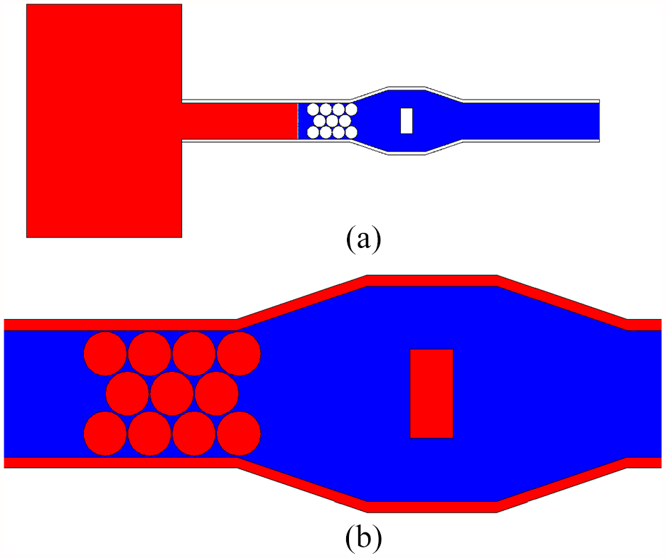
System investigated for multimode thermal and mechanical interaction model development: (a) system studied with region of higher initial pressure and temperature driving the flow and (b) system configuration: initial solid particle positioning, fixed flow path obstruction, and flow path geometry.

With the continued development of machine learning techniques, the methods for the direct flow-particle motion coupled models described in this paper may be used to “train” machine learning–based models and to generate surrogate models. In such a way, estimates of the localized interface conditions and resulting effects such as forces and heat transfer can be simulated with greater detail than the standard modeling techniques, but with reduced computational intensity compared to the direct coupling presented in this work, particularly for high particle count flows. The studies by Balachandar et al.³⁰ and Ganti and Khare³¹ are two early applications of machine learning–based techniques that demonstrate such methods may serve as an avenue for more detailed computational modeling of multiphase flow conditions without the heavy computational requirements associated with directly modeling each particle within the flow. For high concentration and frequent particle interaction conditions, the techniques described in the current work may serve as the foundation for creating such surrogate type models. Again, the machine learning algorithms will not provide the same fidelity as the direct discretization, but may reduce overall computational requirements for conditions with high particle concentrations and where more details are required than can be obtained from standard modeling methods.

2. Methodology

The direct moving particle mechanical–thermal interaction modeling method implements a combination of the modeling techniques developed in previous works by the author as described in Florio^1–6 for expanded capabilities. The basic methodology of this combined technique is summarized below with the major components being contact determination, the specification of the mechanical interaction effects, the specification of the thermal interaction effects, and the specification of the motion of the objects in the system.

2.1. Contact determination

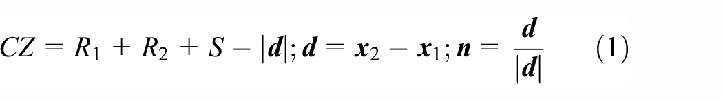
While the fluid–particle interactions are continuously captured, particle–particle or particle–solid interactions are only activated for the solid bodies that are in contact. In this work, the particles are circular for the two-dimensional models used to demonstrate the methodology, but the techniques are equally appropriate for three-dimensional spherical particles. For circular particle–particle contact to occur, CZ as defined in Equation (1) must be greater than zero. This statement is equivalent to requiring the distance between the centroids of the two particles be less than the sum of the two particle radii and a safety zone thickness, S, as shown in Figure 2. The safety zone, S, maintains the mesh topology in the system, R₁ is the radius of particle 1, R₂ is the radius of particle 2, and x ₁ and x ₂ are the centroids of particle 1 and particle 2, respectively. A vector d is directed from the centroid of particle 1 to the centroid of particle 2, with the vector n defined as the unit vector in the d direction:

CZ = R_{1} + R_{2} + S - | d |; d = x_{2} - x_{1}; n = \frac{d}{| d |}

(1)

Figure 2.

Interacting particle geometry.

A Hertz contact model–based contact area and contact length are assumed.^4,5,30,31 Further details can be found in Florio,^4,5 Balachandar et al.,³⁰ and Ganti and Khare.³¹

2.2. Mechanical interaction model

The mechanical interaction model for a given particle involves two components, the contact effects which are active only for objects in contact and the fluid forces which are always at work. Once a set of particles/objects is identified as contacting, a soft collision mechanical interaction model is used to replicate the effects of the mechanical contact. The contact force and moment formulation is derived from those described in Matuttis and Chen³² and Marshall and Li.³³ The spring and damper-based contact forces acting on particle 1 are listed below, with oppositely directed forces acting on particle 2. The normal force is as follows:

{\bar{F}}_{n} = - (K_{N} + G_{N} (\bar{n} \cdot {\bar{v}}_{R})) \bar{n}

(2)

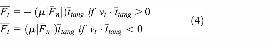
The force in the tangential direction is as follows:

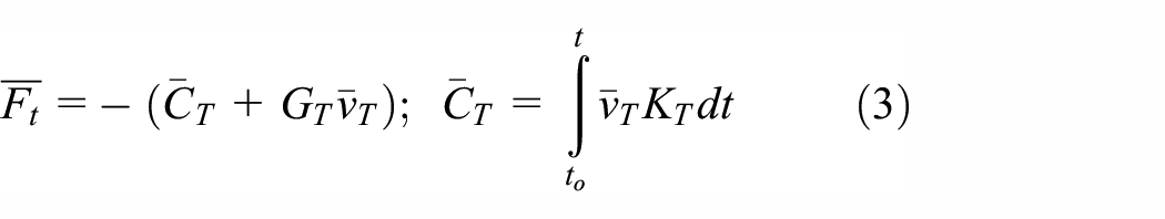
\bar{F_{t}} = - ({\bar{C}}_{T} + G_{T} {\bar{v}}_{T}); {\bar{C}}_{T} = \int_{t_{o}}^{t} {\bar{v}}_{T} K_{T} dt

(3)

If the magnitude of $\bar{F_{t}}$ is greater than the critical force, $μ | {\bar{F}}_{n} |,$ then the force above is replaced by:

\begin{matrix} \bar{F_{t}} = - (μ | {\bar{F}}_{n} |) {\bar{t}}_{tang} if {\bar{v}}_{t} \cdot {\bar{t}}_{tang} > 0 \\ \bar{F_{t}} = (μ | {\bar{F}}_{n} |) {\bar{t}}_{tang} if {\bar{v}}_{t} \cdot {\bar{t}}_{tang} < 0 \end{matrix}

(4)

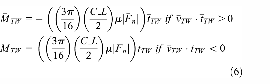
The following moments acting on particle 1 are also defined. ${\bar{M}}_{TW}$ is the twisting moment:

{\bar{M}}_{TW} = - ({\bar{C}}_{TW} + G_{TW} {\bar{v}}_{TW}); {\bar{C}}_{TW} = \int_{t_{o}}^{t} {\bar{v}}_{TW} K_{TW} dt

(5)

If $| {\bar{M}}_{TW} |$ is greater than the critical moment, $(3 π / 16) (C_L / 2) μ | {\bar{F}}_{n} |,$ then the moment above is replaced by:

\begin{matrix} {\bar{M}}_{TW} = - ((\frac{3 π}{16}) (\frac{C_L}{2}) μ | {\bar{F}}_{n} |) {\bar{t}}_{TW} if {\bar{v}}_{TW} \cdot {\bar{t}}_{TW} > 0 \\ {\bar{M}}_{TW} = ((\frac{3 π}{16}) (\frac{C_L}{2}) μ | {\bar{F}}_{n} |) {\bar{t}}_{TW} if {\bar{v}}_{TW} \cdot {\bar{t}}_{TW} < 0 \end{matrix}

(6)

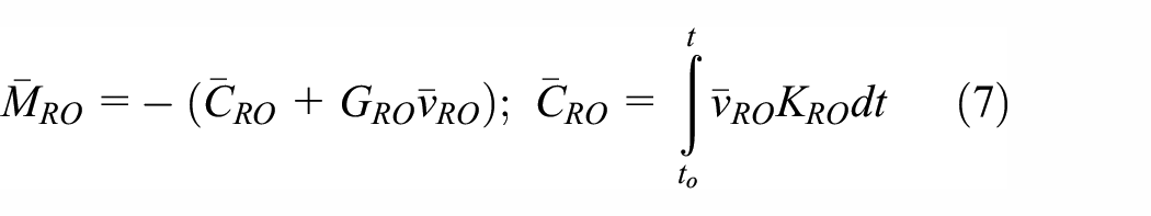
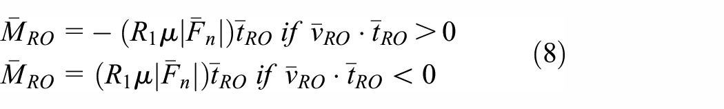
A rolling contact moment is given by:

{\bar{M}}_{RO} = - ({\bar{C}}_{RO} + G_{RO} {\bar{v}}_{RO}); {\bar{C}}_{RO} = \int_{t_{o}}^{t} {\bar{v}}_{RO} K_{RO} dt

(7)

If $| {\bar{M}}_{RO} |$ is greater than the critical moment, $R_{1} μ | {\bar{F}}_{n} |,$ then the moment above is replaced by:

\begin{matrix} {\bar{M}}_{RO} = - (R_{1} μ | {\bar{F}}_{n} |) {\bar{t}}_{RO} if {\bar{v}}_{RO} \cdot {\bar{t}}_{RO} > 0 \\ {\bar{M}}_{RO} = (R_{1} μ | {\bar{F}}_{n} |) {\bar{t}}_{RO} if {\bar{v}}_{RO} \cdot {\bar{t}}_{RO} < 0 \end{matrix}

(8)

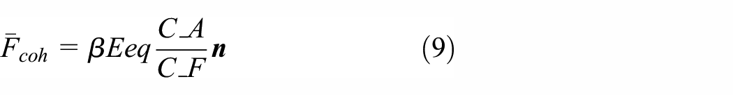
A cohesive force can also be defined as from Matuttis and Chen³² with a value of β varied:

{\bar{F}}_{coh} = β Eeq \frac{C_A}{C_F} n

(9)

Further details on the specific coefficient and parameter formulations can be found in Florio:⁴

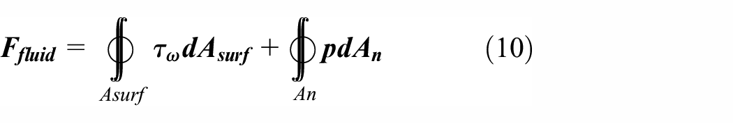
F_{fluid} = \underset{Asurf}{∯} τ_{ω} d A_{surf} + \underset{An}{∯} pd A_{n}

(10)

The fluid-induced forces acting on a solid body can also be calculated, including the pressure and viscous forces as in Equation (10).

The localized nature of the flow generates localized forces acting on the system components, altering the moving object trajectory and thus the coupled flow. With larger particle sizes and smaller distances between the particles or other system components, the variation in the flow conditions around a particle and the coupled flow-object motion is therefore important in appropriately modeling the system conditions.

2.3. Thermal interaction model

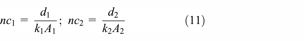
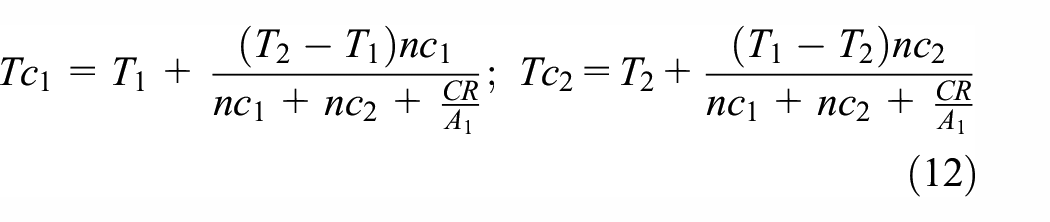
Similarly, the thermal interaction models include the conductive contact model active only for contacting objects and the fluid–particle and radiation models which are always active. Conduction contact is estimated through a novel technique introduced in Florio⁵ that maintains a fluid gap space at the fluid–solid interfaces. Such a gap space is needed to retain the original mesh topology and prevent mesh overlap in the computational flow domain. An area weighted average temperature over the contacting cells on each particle, T₁ and T₂, and an area weighted average normal distance from the boundary surface to each “contacting” cell centroid, d₁ and d₂, are calculated. These parameters along with the contact area, A₁ and A₂, and a contact resistance, CR, are used to formulate a contact surface temperature at each object, T_c₁, and T_c₂. Further details can be found in Florio:⁵

n c_{1} = \frac{d_{1}}{k_{1} A_{1}}; n c_{2} = \frac{d_{2}}{k_{2} A_{2}}

(11)

T c_{1} = T_{1} + \frac{(T_{2} - T_{1}) n c_{1}}{n c_{1} + n c_{2} + \frac{CR}{A_{1}}}; T c_{2} = T_{2} + \frac{(T_{1} - T_{2}) n c_{2}}{n c_{1} + n c_{2} + \frac{CR}{A_{1}}}

(12)

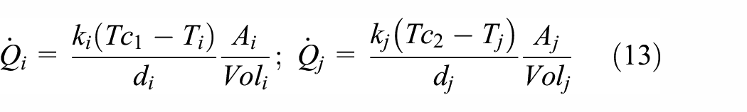
The conduction contact temperatures are reformulated into a volumetric energy source at each computational cell (Equation (13)), allowing local temperature variation along the contact zone on each particle. In Equation (13), cell i on particle 1 has a volume Vol_i and cell j on particle 2 a volume Vol_j. See Florio⁵ for more information:

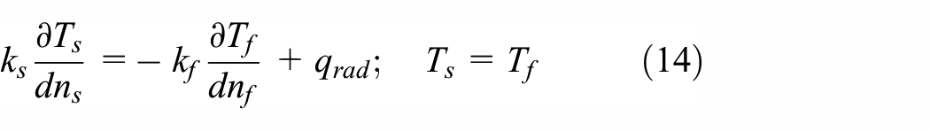
{\overset{\cdot}{Q}}_{i} = \frac{k_{i} (T c_{1} - T_{i})}{d_{i}} \frac{A_{i}}{Vo l_{i}}; {\overset{\cdot}{Q}}_{j} = \frac{k_{j} (T c_{2} - T_{j})}{d_{j}} \frac{A_{j}}{Vo l_{j}}

(13)

The convective heat exchange at the fluid–solid interfaces is continuously active. The local flow and temperature conditions are used to ensure conservation of energy and equivalency of temperatures at the interfaces. In Equation (14), f indicates fluid and s indicates solid. See Florio^5,6 for further details:

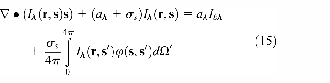
k_{s} \frac{\partial T_{s}}{d n_{s}} = - k_{f} \frac{\partial T_{f}}{d n_{f}} + q_{rad}; T_{s} = T_{f}

(14)

With the discretization of the particles and flow paths, the local geometry and temperature field data can be used as input into models for the continuous thermal radiation exchange between solid surfaces and between solid surfaces and the fluid. The Discrete Ordinates (DO) model is implemented with the assumption that all solid bodies are opaque, diffusive, gray bodies, though these assumptions are not tied to the DO method. The governing equation for the DO model (Equation (15)) is solved in a manner similar to the momentum and energy equations in the fluid for fixed number of direction vectors, s:³⁴

\begin{matrix} \nabla • (I_{λ} (r, s) s) + (a_{λ} + σ_{s}) I_{λ} (r, s) = a_{λ} I_{b λ} \\ + \frac{σ_{s}}{4 π} \int_{0}^{4 π} I_{λ} (r, s') φ (s, s') d Ω' \end{matrix}

(15)

$I_{λ} (r, s)$ is the spectral intensity λ is the wave length, $a_{λ}$ spectral absorption coefficient, $I_{b λ}$ is the black body intensity, $σ_{S}$ is the scattering coefficient, $φ (s, s')$ is the phase function, $Ω'$ is the solid angle, and s′ is the scattering direction vector.

With the variation in the temperature fields within particles or other objects and within the fluid flow surrounding the particles or other objects commonly found in the flow conditions of interest, the phenomena including conduction within the particles, the conjugate heat transfer at the flow–solid interfaces and the radiation exchange between surfaces (or with the gases) cannot be simply neglected or adequately modeled through a lumped temperature model, particularly if temperature is driving the phenomena of interest in an investigation.

2.4. Object motion calculation

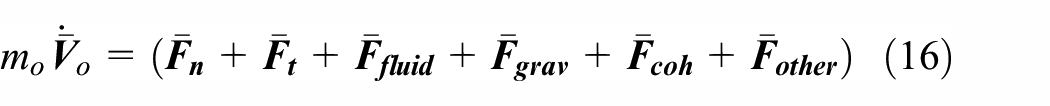
The translational motion of each object is found from the conservation of linear momentum. The normal and tangential contact forces, F_n and F_t , and the fluid induced force, F_fluid , along with any additional forces including the gravitational and cohesion forces can be considered when calculating the translational motion of each moving object. The linear acceleration, ${\bar{V}}_{o}^{.}$ , from which the velocity and displacement of each object are found is given in Equation (16):

m_{o} {\dot{\bar{V}}}_{o} = ({\bar{F}}_{n} + {\bar{F}}_{t} + {\bar{F}}_{f l u i d} + {\bar{F}}_{g r a v} + {\bar{F}}_{c o h} + {\bar{F}}_{o t h e r})

(16)

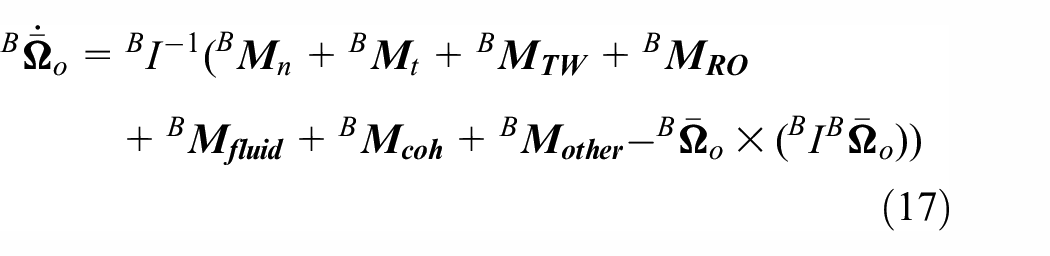
The rotational motion of each object can be calculated in a similar manner. A quaternion-based formulation is adopted due to the potential for high rotation rates under high speed flow or particle motion. Further details on this formulation can be found in Shames,³⁵ Ickes,³⁶ and Florio.⁴ For an object with a local body coordinate system, B, a global coordinate system, G, and local coordinate system based moment of inertia, ^BI, the local coordinate system-based angular acceleration, ${}^{B}{\overset{\cdot}{\bar{Ω}}}_{o}$ , can be found. All moments must be transformed to the local coordinate system B in Equation (17), but a final transformation of the motion vectors/parameters to the global coordinates is needed:

\begin{matrix} {}^{B}{\overset{\cdot}{\bar{Ω}}}_{o} =^{B} I^{- 1} (^{B} M_{n} +^{B} M_{t} +^{B} M_{TW} +^{B} M_{RO} \\ +^{B} M_{fluid} +^{B} M_{coh} +^{B} M_{other} -^{B} {\bar{Ω}}_{o} \times (^{B} I^{B} {\bar{Ω}}_{o})) \end{matrix}

(17)

2.5. Determination of conditions within the system gas and solids

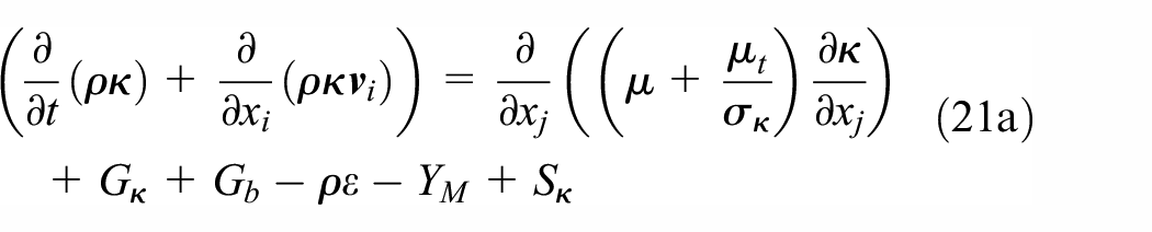
The flow and thermal conditions in the fluid and particles/solids can be determined numerically, incorporating any of the interaction and particle motion effects described above. An ideal gas equation of state and κ−ε turbulence model are implemented for the gas flow in the current investigation, though the method is not restricted to this selection. The governing equations for a single phase flow are as follows.

The differential equation governing the conservation of mass:³⁷

\partial ρ / \partial t + \nabla \cdot (ρ \bar{v}) = 0

(18)

The vector-based partial differential equation governing the conservation of momentum is given by:³⁷

ρ D \bar{v} / Dt = \nabla \cdot τ_{ij} - \nabla p

(19)

The equation governing the conservation of energy is expressed as:³⁷

ρ Dh / Dt = Dp / Dt + \nabla \cdot (k \nabla T) + τ_{ij} \partial v_{i} / \partial x_{j}

(20)

The two equations below govern the two turbulence parameters in the κ−ε realizable model:³⁸

\begin{matrix} (\frac{\partial}{\partial t} (ρ κ) + \frac{\partial}{\partial x_{i}} (ρ κ v_{i})) = \frac{\partial}{\partial x_{j}} ((μ + \frac{μ_{t}}{σ_{κ}}) \frac{\partial κ}{\partial x_{j}}) \\ + G_{κ} + G_{b} - ρ ε - Y_{M} + S_{κ} \end{matrix}

(21a)

\begin{matrix} (\frac{\partial}{\partial t} (ρ ε) + \frac{\partial}{\partial x_{i}} (ρ ε v_{i})) = \frac{\partial}{\partial x_{j}} ((μ + \frac{μ_{t}}{σ_{ε}}) \frac{\partial ε}{\partial x_{j}}) \\ + ρ C_{1} S_{ε} ε - ρ C_{2} \frac{ε^{2}}{κ + \sqrt{ε μ / ρ}} + C_{1 ε} \frac{ε}{κ} C_{3 ε} G_{b} + S_{ε} \end{matrix}

(21b)

The equation governing the conservation of energy in the solid bodies includes a general energy source without any flow or convective effects:²⁵

d (ρ c_{p} T) / dt = \nabla \cdot (k \nabla T) + \overset{\cdot}{Q}

(22)

2.6. Material properties

The gas fluid used in this work is air and the air is treated as an ideal gas with a kinetic theory–based viscosity and thermal conductivity and the temperature-dependent specific heat from McBride et al.³⁹

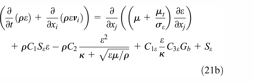
All solid entities are given constant material property values as described in specific parameter cases studied in Table 1. The material properties are customizable so that temperature-dependent material properties or material properties that variation among the particles can readily be assigned.

Table 1.

Tank pressure and temperature and particle/flow path surface emissivity cases considered.

Parametervaried	Case	Thermal conductivity	Specificheat	Density	Cohesion parameter	Young’smodulus	Bulkmodulus	Tankpressure	Emissivity
Parametervaried	Case	k (W/m K)	cp(J/kg K)	ρ (W/m³)	β	E (Pa)	G (Pa)	(Pa)	ε
Density	1	202.4	871	800	1.50E–04	1.00E + 11	2.00E + 10	4.00E + 07	0
	2	202.4	871	1600	1.50E–04	1.00E + 11	2.00E + 10	4.00E + 07	0
	3	202.4	871	3200	1.50E–04	1.00E + 11	2.00E + 10	4.00E + 07	0
	4	202.4	871	6400	1.50E–04	1.00E + 11	2.00E + 10	4.00E + 07	0
Cohesion	5	202.4	871	800	0	1.00E + 11	2.00E + 10	4.00E + 07	0
	6	202.4	871	800	1.50E–05	1.00E + 11	2.00E + 10	4.00E + 07	0
	1	202.4	871	800	1.50E–04	1.00E + 11	2.00E + 10	4.00E + 07	0
	7	202.4	871	800	1.50E–03	1.00E + 11	2.00E + 10	4.00E + 07	0
Specific heat	8	202.4	8.7	800	1.50E–04	1.00E + 11	2.00E + 10	4.00E + 07	0
	9	202.4	87.1	800	1.50E–04	1.00E + 11	2.00E + 10	4.00E + 07	0
	1	202.4	871	800	1.50E–04	1.00E + 11	2.00E + 10	4.00E + 07	0
Thermal conductivity	10	2.024	8.7	800	1.50E–04	1.00E + 11	2.00E + 10	4.00E + 07	0
	11	20.24	87.1	800	1.50E–04	1.00E + 11	2.00E + 10	4.00E + 07	0
	1	202.4	871	800	1.50E–04	1.00E + 11	2.00E + 10	4.00E + 07	0
Young’s modulus	12	202.4	871	800	1.50E–04	1.00E + 10	2.00E + 10	4.00E + 07	0
	13	202.4	871	800	1.50E–04	5.00E + 10	2.00E + 10	4.00E + 07	0
	1	202.4	871	800	1.50E–04	1.00E + 11	2.00E + 10	4.00E + 07	0
	14	202.4	871	800	1.50E–04	2.00E + 11	2.00E + 10	4.00E + 07	0
Pressure	1	202.4	871	800	1.50E–04	1.00E + 11	2.00E + 10	4.00E + 07	0
	15	202.4	871	800	1.50E–04	1.00E + 11	2.00E + 10	8.00E + 07	0
	16	202.4	871	800	1.50E–04	1.00E + 11	2.00E + 10	1.20E + 08	0
Radiation	17	202.4	871	800	1.50E–04	1.00E + 11	2.00E + 10	4.00E + 07	0
Radiation	18	202.4	871	800	1.50E–04	1.00E + 11	2.00E + 10	4.00E + 07	1.00

2.7. Numerical implementation

The modeling technique developed is implemented by coupling the commercial code FLUENT^© to a set of customized C subroutines that contain the specific interaction techniques and methods described. The fundamental governing equations in Equations (18) and (22) are solved within FLUENT^© and FLUENT^© is used to move the particles or other objects through the fluid by the specified translational and rotational displacements.

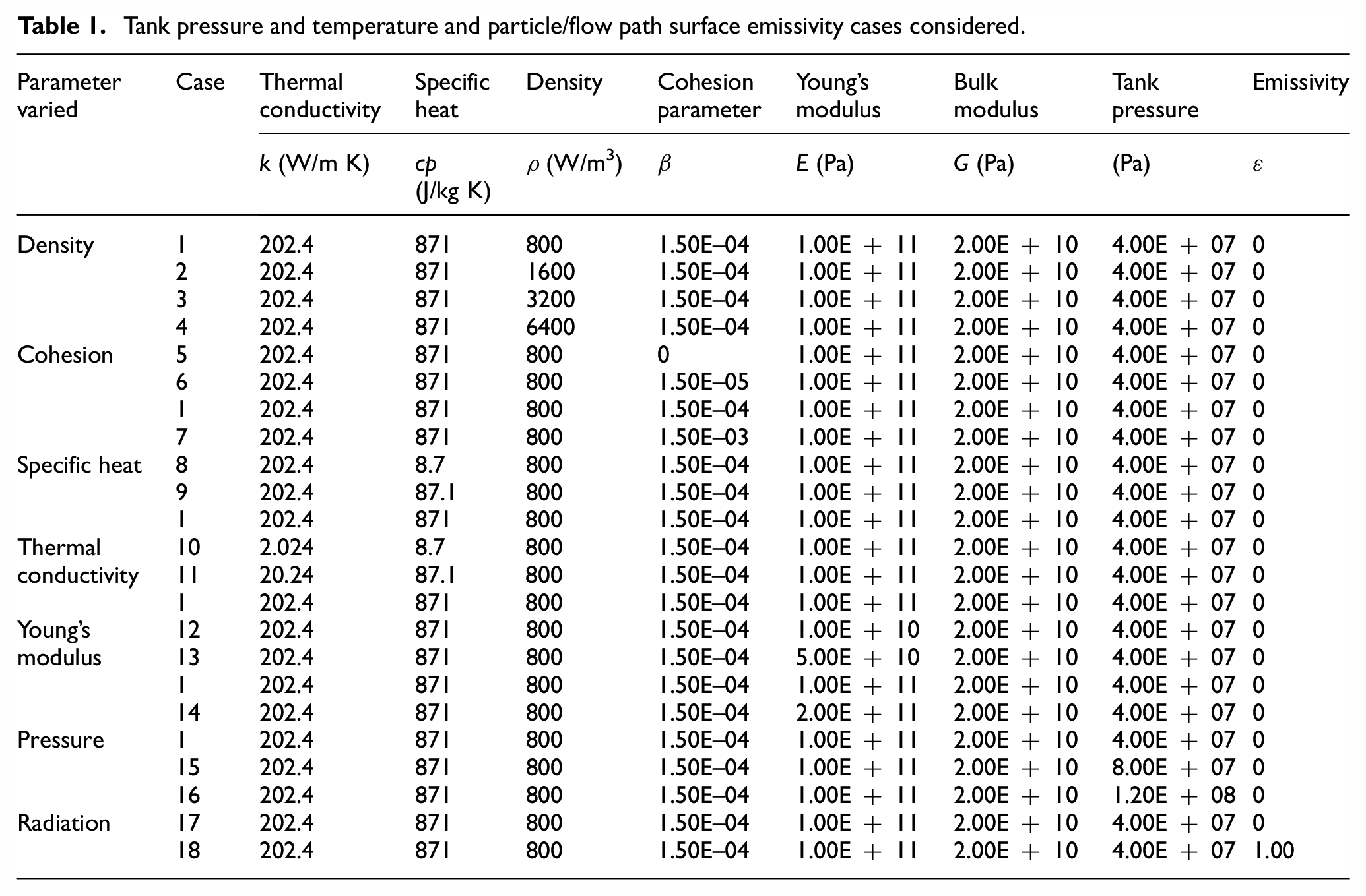
To demonstrate the combined modeling methods in a timely fashion, two-dimensional simulations of the system in Figure 1 are conducted in this work. A triangular mesh is used in the bulk material with quadrilateral elements at the boundary layer at the interfaces between the solid and the fluid. The quadrilateral elements provide more stable and accurate results for the contact heat conduction, while the triangular elements are required for the free object motion. The final mesh used in this study, at the initial particle positions, is shown in Figure 3. Sixty-four elements are present around the circumference of each particle and the flow channel length is composed of 210 elements with a total of 300,000 elements. A mesh sensitivity study was conducted for the baseline Case 8 in Table 1, comparing the particle boundary temperature distribution at 0.1 ms from the start of the simulation. Doubling the element count in Figure 3 results in only a maximum 1.5% change in the local temperatures.

Figure 3.

Mesh: (a) overall and (b) near boundary.

An implicit solution method in time and space is implemented. A Green-Gauss node-based gradient discretization is used with second-order pressure coupling, second-order upwind discretization for the pressure, density, momentum, energy, turbulence parameters, and the Discrete Ordinates equation and second-order discretization in time. A PISO pressure–velocity coupling is assigned. The time step is set to 1.0e–08 s for this compressible flow problem. The simulations were run on a 36 core processor Linux machine utilizing 72 processors. The simulations required approximately 48 h to reach 0.015 s, with the radiation cases requiring a longer run-time of 72 h to reach the same terminal time.

The results produced by the mechanical and thermal interaction components of the modeling methods were compared to the results of the same system and phenomena using traditional modeling methods of mechanical contact and thermal interaction, respectively, devoid of any fluid flow. The good comparison of results provides justification for the use of these methods in the current work. The particle motion predicted by the mechanical interaction model for a two-particle contact closely follows the motion predicted from a finite-element elastic and elastic–plastic material model of the same particle collision event as in Figure 4(a).¹ The temperature distribution across the centerline of two contacting particles for the current modeling technique (marked with triangles) and a standard finite volume heat conduction across the contacting particles are compared in Figure 4(b).⁵

Figure 4.

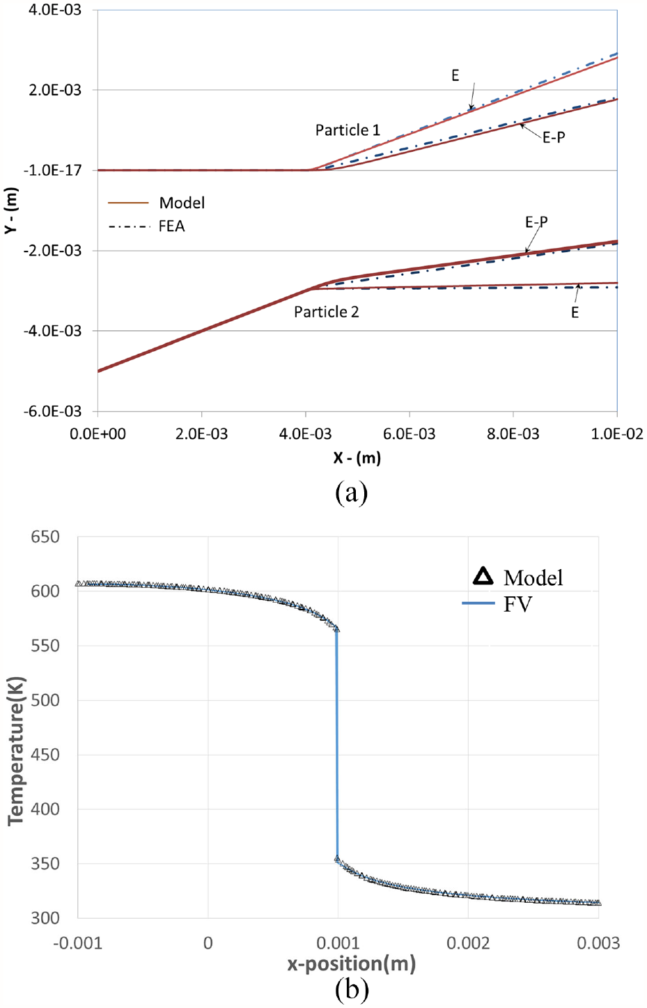
Comparisons between current modeling method components and standard modeling techniques: (a) mechanical contact model comparison and (b) conductive contact model comparison.

3. Problem statement

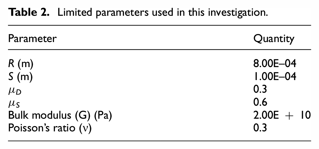
The utility of the innovative combination thermal and mechanical interaction moving particle–fluid flow modeling technique described in this paper is demonstrated through the modeling and analysis of the system shown in Figure 1, involving 12 moving and interacting particles of a large size relative to the flow path and high pressure, and high temperature gas. The high pressure gas is initially contained in the tank on the left, shown in red in Figure 1(a) (see online version for color) and once released, the gas flows around the 12 initially in-line particles, with a flow obstruction instigating more vigorous particle interactions. Each row of particles is initially assigned a different temperature to ensure the occurrence of thermal interactions can be readily visualized and captured in the simulations to highlight the modeling capabilities, with the upper row of particles given an initial temperature of 1380 K, the mid row 920 K, and the lower row 460 K. The particle radii are 0.80 mm (Table 2). The particles are numbered left to right, 0 through 3 in the lower, cold row, 4 through 7 in the mid row, and 8 through 11 in the upper row at the highest temperature. The safety zone clearance, S, the static and dynamic friction coefficients, and the bulk modulus and Poisson’s ratio are provided in Table 2. A simple elastic mechanical interaction model is implemented and no thermal contact resistance is applied.

Table 2.

Limited parameters used in this investigation.

Parameter	Quantity
R (m)	8.00E–04
S (m)	1.00E–04
µ_D	0.3
µ_S	0.6
Bulk modulus (G) (Pa)	2.00E + 10
Poisson’s ratio (ν)	0.3

3.1. Parameters varied

To illustrate the function of the modeling method over a range of system parameters, sensitivity studies varying the parameters in Table 1 are performed to compare the flow and thermal conditions. The parameters varied include the particle density, specific heat, thermal conductivity, Young’s modulus, the cohesion factor, β, from Equation (9), the initial driving tank pressure, P, and the radiation conditions of the particle/flow path surfaces.

3.2. Boundary conditions

All solid boundaries are assigned a no slip boundary condition. The outer bounds of the domain are assigned a pressure outlet boundary condition with the pressure set to 101,325 Pa. The outer surfaces of the “tank” holding the initially high pressure gas and the outside surfaces of the flow path are held insulated. Conjugate heat transfer is simulated at any fluid–solid interfaces. A gray-diffuse body assumption is applied so the emissivity of the solid particle and flow path surfaces must be specified (Table 2) with the transmissivity of the solid materials set to zero. Radiation exchange with the fluid is not considered in this work.

3.3. Initial conditions

The gas in the system is initially at an ambient temperature of 300 K, an ambient pressure of 101,325 Pa, and is at rest. The gas in the tank region is given an initial pressure, 40 MPa for the baseline case, and a temperature of 1500 K. These values are chosen to be sufficient to drive the particle motion and result in gas temperature ranges that vary from the particle temperatures. The κ-turbulence parameter is set to 0.1 initially and the ε turbulence parameter to 10.0. All solids excluding the particles are given an initial temperature of 300 K. From the upper to the lower row, the particles are given an initial temperature of 1380 K, 920 K, and 460 K, respectively. To amplify the effects of radiation, when radiation is considered, the initial particle temperatures are raised to 2300 K, 930 K, and 300 K (Table 1).

4. Description of the results

The results of the parametric studies conducted for the 12 particle system with the flow obstruction expose the utility of the new modeling method as well as provide insight into the localized particle-laden flow phenomena. In this section, the flow and temperature field patterns for a representative case (Case 8, Table 1) are traced over time to highlight the effects that can be observed with the modeling technique. The online version of this paper contains an animated version of the temperature field contours for the Case 8, Table 1. Then, the effects of varying each of the parameters as listed in Table 1 are described.

4.1. Representative results and description of phenomena

Since the thermal interactions are more intense and visible with the lower specific heat values, Case 8 with the lowest specific heat was selected for a more detailed discussion of the local thermal effects that develop in the particle-laden flow. As the gas flow approaches the particles, the gases slow and the kinetic energy is used to increase the temperature and pressure of the gases. The local distribution of the temperature (Figure 5(a)) indicates the high temperatures at the upstream side of the particles (A) and low temperature zones between the particles (B), with the low temperature zone shrinking moving downstream. The effects of conjugate heat transfer to the flow path can be seen at the expansion zone of the flow path below (A). The temperatures within each of the particles can also be seen. High temperatures are found on the upstream side of the particles. Convective heating also contributes to the higher temperature found at the zones diagonal to the flow in the lower row of particles. Conductive contact cooling of the particles (C) and heating of the plate (D) can be observed. The model results show the diversion of the flow streams and blockage effects caused by the upstream particles protects the downstream particles from the extent of the temperature increase as that occurring on the upstream particles. The heating of the flow path, the local variation of temperature within the particle, the localized fluid induced temperature changes in the diverting plate, and the localized cooling and/or heating effects due to specific particle contact with the plate cannot be captured with this level of detail using the DEM-Eulerian-based models or when using simplified solid body thermal models coupled to a CFD model.^12,15–17 The contour plots presented clearly show, qualitatively, the spatial and temporal variation in the temperature and flow fields surrounding and within the particles, flow path surfaces, and the flow obstructing plate and how localized, time-dependent effects such as a specific contact or specific flow stream impingement upon surface contributes to these thermal conditions.

Figure 5.

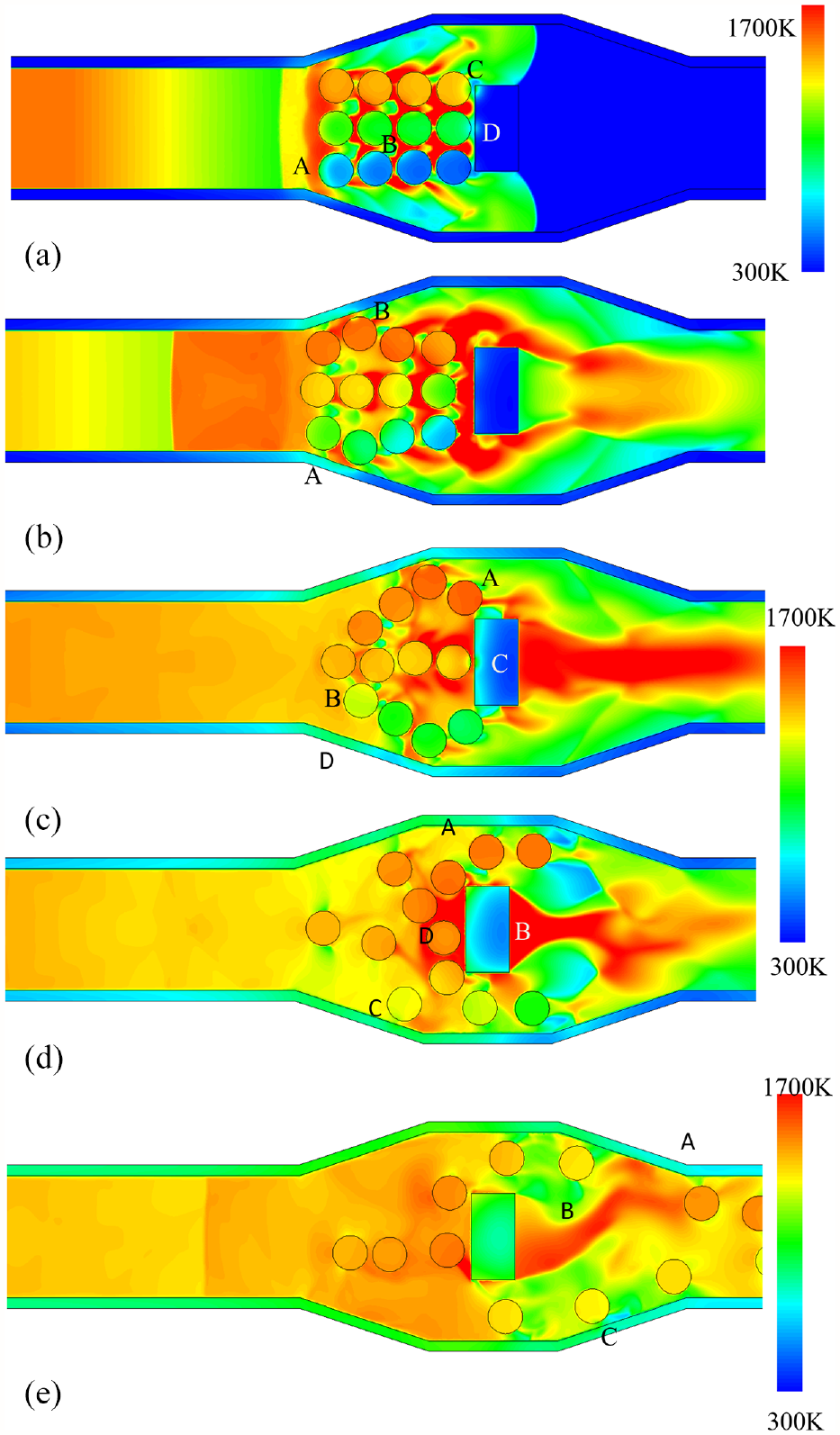
Temperature contour sequence for Case 8, representative temperature features: (a) Time 1, (b) Time 2, (c) Time 3, (d) Time 4, and (e) Time 5.

As the particles move and impact the flow obstructing plate, the particles in the right-most column rebound from the surface, and, as a consequence, are forced to more vigorously interact with the particles that are continuing to move toward the plate, leading to contact between particles from different initial rows at different temperature levels and to changes in the particle positioning. Since the upper and lower rows of particles are less constrained, these particles begin to spread and move closer to the walls (Figure 5(b)). Near area B in Figure 5(b), the yellow region on the particle temperature contour indicates wall contact-based cooling, a localized feature not available with the standard modeling methods, also demonstrating the potential for variation in the temperature and flow field at the fluid–solid interfaces. Continued heating of the particles can be observed at this time, with the upstream zone of a given particle achieving higher temperatures as the higher velocity and higher temperature flow streams move over this portion of the surface. As the particles move, the flow conditions are altered as the positioning and magnitudes of the high speed flow streams change. Thus, the convective-based particle heating also changes with time and location around each particle. A standard modeling method like in Vargas and McCarthy¹² would apply a correlation uniformly at the interface-based heat transfer average flow and particle conditions, rather than accounting for the potential variation in the flow and temperature conditions and therefore the heat transfer coefficient along a surface. Instead, in the current work, the conjugate heat transfer is directly modeled. The local flow, temperatures, and pressures can be accessed to study additional phenomena. These localized effects would not be captured in standard models, making the localized phase change, chemical reactions, or other flow, temperature, or concentration condition dependent effects difficult to model.

As time proceeds, the particle distribution becomes increasingly less orderly and the particles move toward the walls of the flow path. The local gas conditions, in response, change. With a more disperse particle arrangement, the flow restrictions caused by the particles is reduced, leading to more direct impingement of the high speed gas on the upstream or left side of the plate. The flow induced heating of the plate near region C in Figure 5(c) becomes more significant. The plate, though, is still at a lower temperature than the particles, and the cooling of the particle in contact with the plate near area C can be observed in Figure 5(c). Continued conjugate heat transfer between the flow and the flow path walls results in higher flow path temperatures as seen near area D in the same figure. The temperature level and the extent of the elevated temperature regions in the flow path grow with time. At the upper portion of the system, near the end of the expanding portion of the flow path, a noticeable locally lower temperature region develops within the particle due to the contact with the cooler flow path. The particle near B develops a high temperature due to the high speed flow impingement as well as the contact with the two hotter particles from the middle particle row. Such localized, fluid–particle, particle–particle, or other object heat transfer conditions are not possible to simulate using the previous methods. The complex temperature field pattern surrounding and between the particles results from the interdependencies between the particle position, particle motion, and the flow conditions. These interdependencies can be attained in the current modeling technique due to the particle discretization within the computational domain and the mechanical and thermal contact models implemented. Localized variations in the flow and temperature field nearby individual particles cannot be modeled with the standard DEM-Eulerian modeling techniques, so this method provides unique modeling capabilities for conditions when these localized effects are related to phenomena of interest.

The gas flow acting on the particles continues to move the particles downstream and eventually to force the particles around the flow obstructing plate. Since the particle motion around the obstruction opens new gas flow paths, the gas temperature initially decreases as the gas accelerates. The heating of the gas flow path continues as seen in area A in Figure 5(d) and the temperature of the plate continues to rise as it is exposed to the hot gases which are coming to rest on the surface as in area D in Figure 5(d). To the rear or downstream side of the plate, the high temperature region consolidates due to the faster flow moving around the plate and the diversion in the flow caused by the presence of the particles as in area B in Figure 5(d). Contact of the particle near C with the flow path wall produces a cooling effect on the particle as seen by the lower temperature region. With time oscillatory shedding from the rear of the obstruction as in Figure 5(e), area B, the higher temperature gas impinges upon the flow path (Area A, Area C) and the particles (Area B) as the higher velocity flow stream sweeps from one side of the flow path to the other, affecting the local thermal conditions and temperature rise in the flow path and particles. Again, the direct coupling of the flow with the particles and the mechanical and thermal interaction facilitates the study of the localized effects that result in the particle-laden flow conditions.

4.2. Demonstration of localized effects

Variation of the flow and thermal conditions develop in the vicinity of the particle–flow interface as the gas flow moves over the set of particles and the particles interact with each other, the obstruction, and the flow path surfaces as described. Here, more specific qualitative and quantitative information is presented to focus on the localized nature of the flow conditions and heating that typically occur near such interfaces in these particle-laden flows. Capturing the local changes in the flow and thermal conditions at the interface and within the particles and other solids in this way is possible because of the discretization of the particles (as well as the flow obstruction and flow path) within the computational domain in the technique devised.

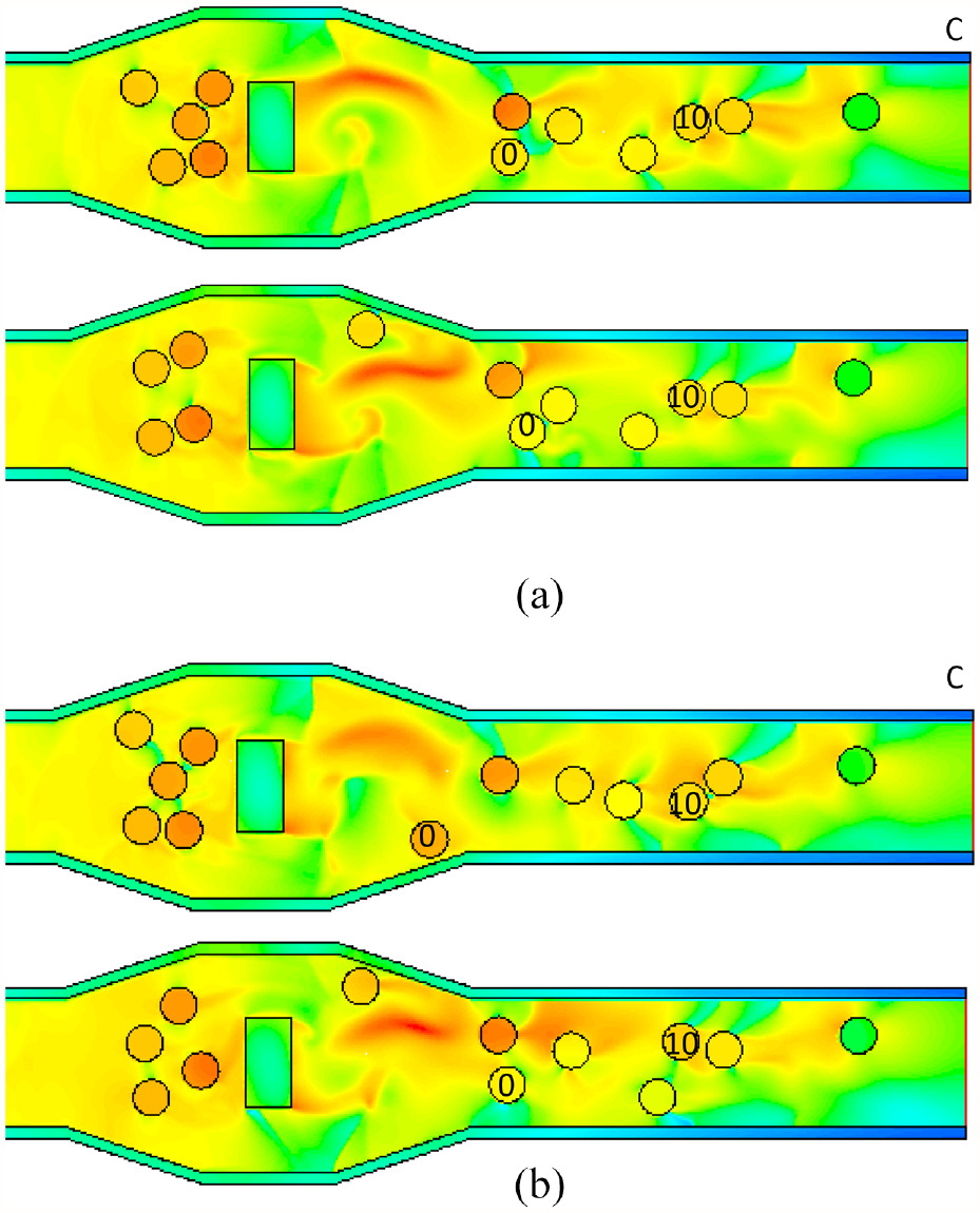
Qualitatively, the time sequence of the temperature field contours in Figure 6 depicts the temperature rise that occurs near the particles as the high speed gas moving left to right begins to impinge upon the particle pack. Because the flow conditions are not uniformly distributed circumferentially about the particle, the flow and temperature fields also vary with the circumferential position around the particles and so vary spatially through the particle material itself (Figure 6(b)–(d)). Since the exterior flow-based heating and the local contact conduction are position dependent, the heat conduction within each particle is also dependent upon location and time, leading to temperatures that continue to vary with radial and angular position. The upstream or left side surface of the particles in the first column receive the main impact of the gas flow, resulting in higher gas temperatures, and higher heating rates on the upstream, left sides of the particles, than on the right side of the particles. The higher velocities moving between the particles due to the flow constrictions generated by the presence of the particle results in higher temperatures skewed to the top side of the particles in the lower row and the bottom side of the particles in the upper row. The spatially dependent temperature distributions within the particles and the flow conditions near the particle–flow interfaces can be seen upon examination of the contour plots in Figure 6. The particle marked 0 for example shows its greatest circumferential variation at the third time in the sequence, with larger variations occurring for downstream particles at later times as the flow conditions change. Hence, non-uniformities in the flow and temperature field occur with particle-laden flow. The regions of greatest variation change with position and time. Since the temporal and spatial distributions of the temperature and flow conditions are available in the current modeling method, the spatial variation in temperature-dependent effects can then be obtained, an important benefit of the modeling method described.

Figure 6.

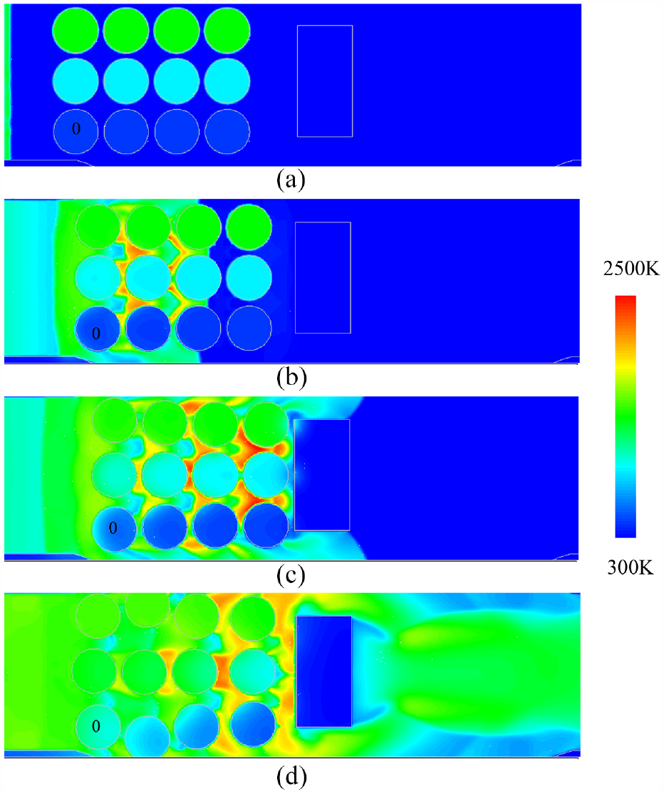
Temperature contour sequence for Case 8, localized temperature effects: (a) Time 1, (b) Time 2, (c) Time 3, and (d) Time 4.

Specific quantitative data can also be used to illustrate the potential spatial variation in key flow and thermal parameters at the particle–flow interface that may occur in the particle-laden flow. Figure 7 presents the pressure, temperature, shear stress, and heat flux about particle 0 (as defined in Figure 6) for four different times labeled 1, 2, 3, and 4. The results clearly show the potential for significant differences in a given quantity with circumferential position and that the extent of this circumferential variation changes with time. For the pressure conditions in Figure 7(a), the pressure can vary by as much as a factor of 7 around the particle interface as seen for time 3. As the flow conditions change, the pressure subsides and while there is still pressure variation around the particle boundary, the variation level is reduced. A similar trend can be found for the temperature in Figure 7(b), where the largest circumferential spatial variation is found at time 3 with a maximum to minimum temperature level of slightly less than 2. At time 4, while a 20% variation in temperature is found, the temperature variation is less significant. With the flow forced between the particles, the flow velocities and flow gradients are highly position dependent as seen in Figure 7(c) which shows the circumferential variation in the shear stress. Again, the largest variation occurs at time 3. Finally, gradients in the temperature field, as shown by the heat flux values at the outer surface of the particle 0, are presented in Figure 7(d). The flux levels at times 2 and 3 are comparable, with the location of the maximum heat flux level shifting as the flow conditions change. At time 4, as the main flow–shock wave has passed over the surface of this particular particle and like the other quantities the heat flux values and variation drop significantly, but the variation that does exist continues to influence the temperature distribution in the particle and any temperature-dependent processes that might develop.

Figure 7.

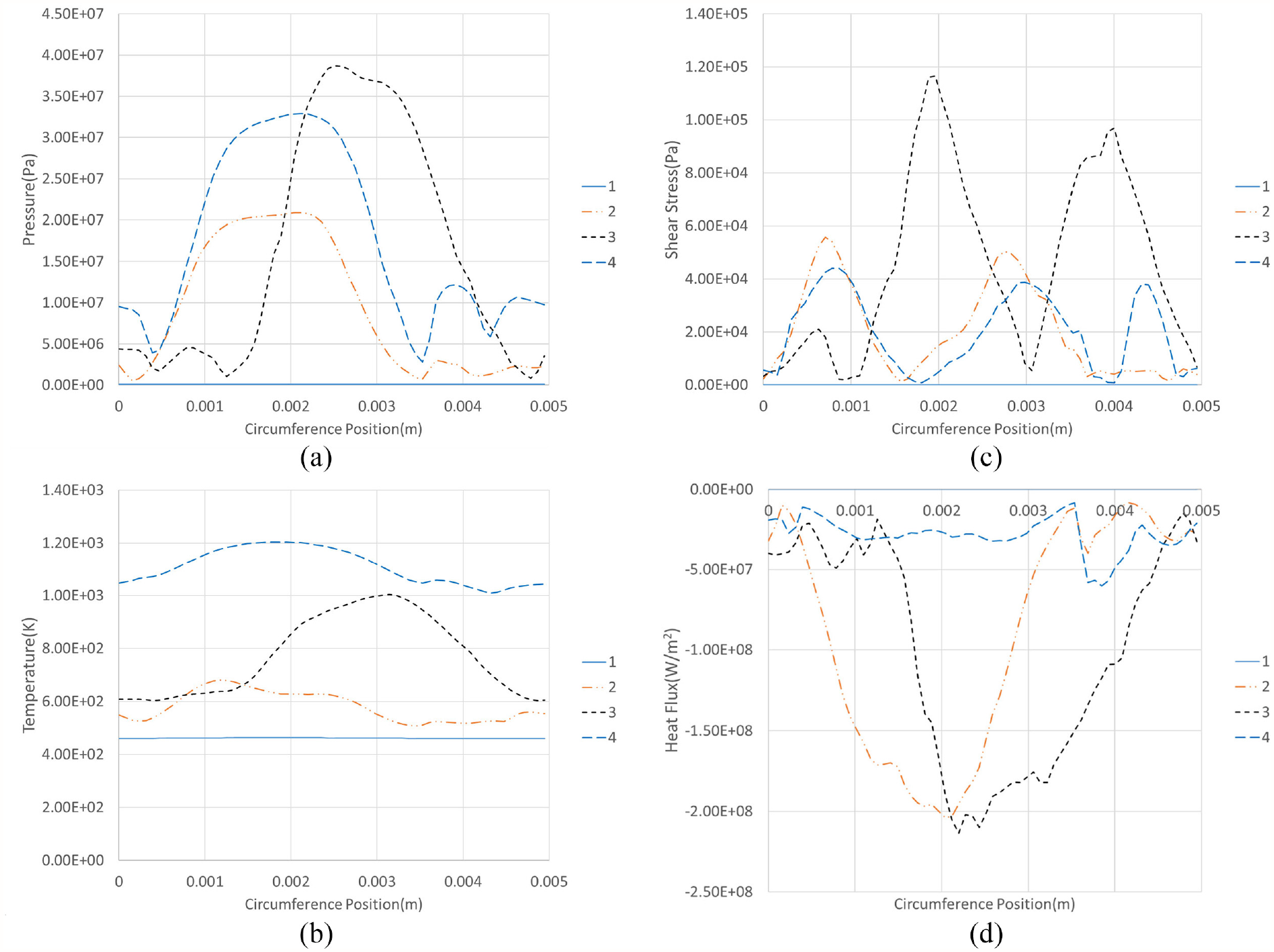
Circumferential variation in quantities indicated at four times. Case 8, localized effects: (a) circumferential pressure distributions, (b) circumferential temperature distributions, (c) circumferential shear stress distributions, and (d) circumferential heat flux distributions.

Based on the results presented and the associated discussion, the following is apparent. Variation about the circumference of a particle or any other object exposed to the high speed gas flow can be captured with the current modeling method. Changes in important flow and thermal quantities about the particle surfaces may not be negligible and can be important in setting the flow and temperature field within the particle-laden flow. The variation in the interface conditions promotes non-uniform temperatures within the particles or other solid objects in the system. If phase changes, chemical reactions, material property dependencies, or other conditions related to the temperature field or flow field are of interest, the modeling method developed provides new capabilities to now consider these events and their local development emanating from the local conditions at the solid–fluid interfaces.

4.3. Effect of particle density

The influence of the system parameters can also be obtained from the simulation results. The density is considered first and the density influences the mass of the particles and the thermal mass or net heat capacity of the particles as well. A larger force is required to cause the same acceleration in a more massive particle than a lighter particle. A higher thermal capacity material which can result from a higher density material produces a lower temperature rise for the same heat input compared with that of a lower thermal capacity material. In this work, the particle density is varied to two, four, and eight times the nominal quantity (Cases 1–4, Table 1). To represent the effects of the density on the motion and temperature field, the surface average temperature of particle 0, the particle initially on the lower left of the pack, and the diverging converging segment of the lower wall of the flow path are traced over time (Figure 8). Temperature contours at approximately 6.0e–05 s are presented in Figure 9.

Figure 8.

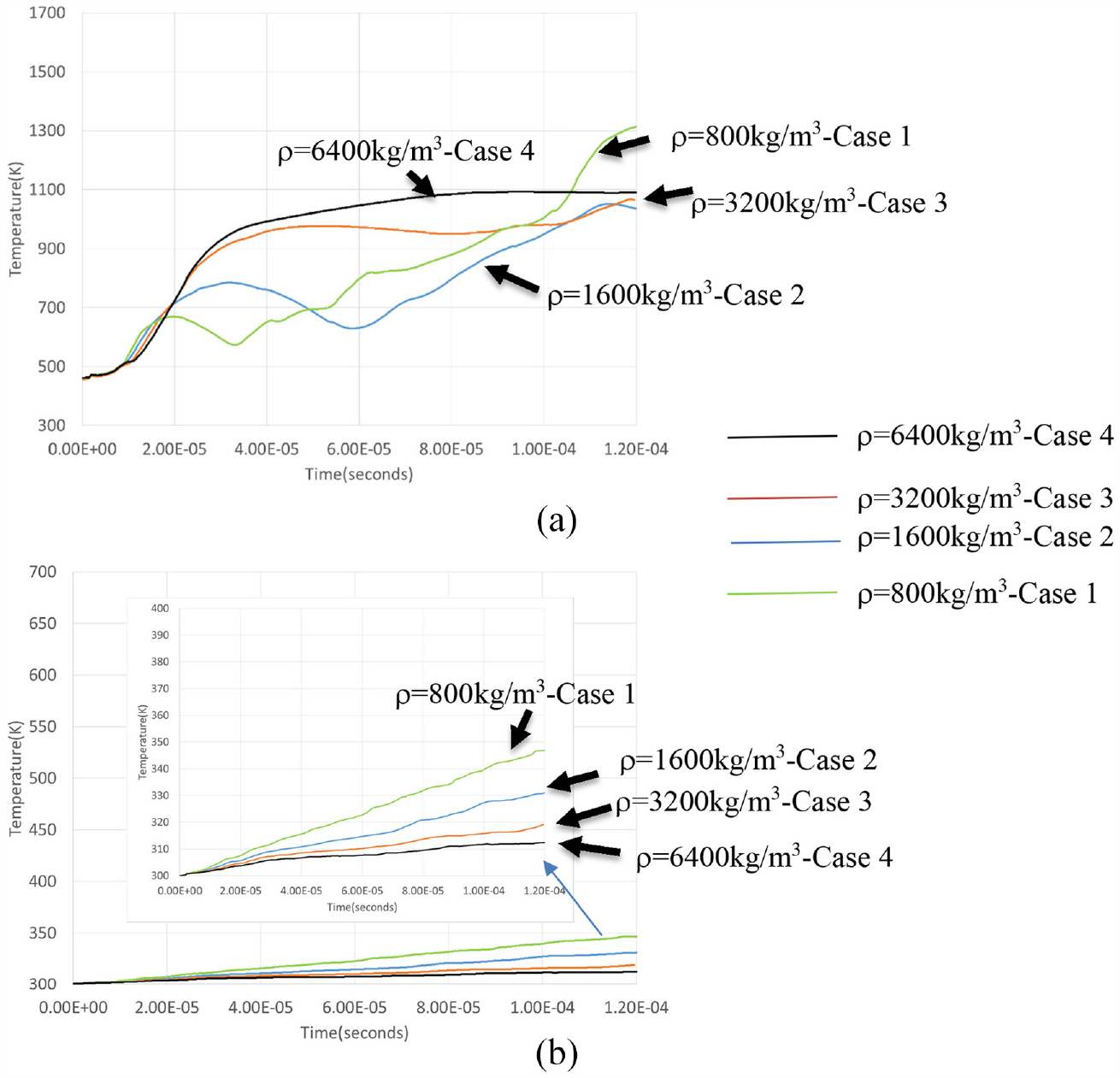
Average temperatures of the entities indicated as the density of the solid material is altered: (a) average temperature of particle 0 and (b) average temperature at lower flow path.

Figure 9.

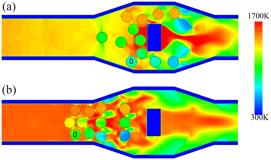
Temperature contour at 6.0e–05 s for the two density cases (Case 1 and Case 4): (a) case of ρ = 800 kg/m³ (Case 1) and (b) case of ρ = 6400 kg/m³ (Case 4).

For the cases studied, the lower density, lighter particles of the same size accelerate faster than the higher density, heavier particles, when subjected to the same initial flow conditions. Because of the differing motion of the particles of different density, excluding the initial impact of the flow on the particles, the fluid induced forces acting on the particles as well as the particle positioning will differ. In Figure 8(a), the temperatures of particle 0 indicate an initial temperature rise for all densities, caused by the kinetic to thermal energy transfer in the decelerating gas flow impinging on the particle. The faster moving, lighter particles impact the flow obstructing plate earlier and begin to move away from the ordered array arrangement sooner than the heavier particles. Hence, for the lighter particles, the flow restrictions caused by the array therefore are lifted at an earlier time, leading to the earlier and sharper rise in the temperature among the four density cases studied as seen in Figure 8(a). The individual particle contacts that can be captured using this modeling method can lead to abrupt, local changes in the temperature of the particle, allowing for the underlying variations in the temperatures and flow to be observed. The model results allow for the underlying causes for these observations to be better understood. For example, for the 800 kg/m³ density case at about 3.5e–05 s, a rise in temperature commences after a time span of falling temperatures (Figure 8(a)). This time corresponds to contact between this particle and two higher temperature particles from the mid-row and the changes are due to the local effects of the contact. Near the end of the time period studied, the particle 0 temperatures for the lowest density case rise above those of the highest density case due to the convective heating resulting from the exposure of the particle surface to the high temperature gases to the rear of the obstruction for these specific conditions. The information gained from the models and the utility of this data in understanding the particle-laden flow condition is an advantage of the current modeling method.

Since the more dense particles move at a slower rate, the heavier particles are exposed to the brunt of the incoming gas flow for a longer period of time. Even post initial contact with the flow obstructing plate, the particles, instead of moving around the flow obstruction, rebound and begin to move upstream. These conditions allow convective heat input to the heavier particles for a longer time, resulting in higher temperatures. The lack of temporal variation in the temperature, beyond the rise in the temperature, due mainly to the gas flow, is a result of the limited particle–particle contact, limited changes in the flow conditions as high speed flow streams touch the surface of the particles, and the increased thermal capacity of the material. A sample of the differences in the motion of the particles and the resulting temperature distributions for the minimum and maximum particle density studied is shown in Figure 9. The particle interactions described and the resulting flow and temperature field data could not be gleaned from a standard particle flow model.

The flow path conditions are also different as the material density changes. The flow path surface reaches a 12% higher temperature with the lower density material due to the lower thermal storage capacity as in Figure 8(b). Just as with the particle temperature condition, the lower rate of oscillations in the wall temperature for the higher density case is in part due to the higher thermal capacity of the material and reduced particle contact.

The interdependencies between the gas flow, the particle positioning, and the temperature field can be readily obtained from the results of the simulations using the method introduced in this work. In addition, the contour plots for this set of results demonstrates the potential local variations in the flow and temperature conditions around the solid–fluid interfaces that can be obtained only with the particles discretized in the flow domain.

4.4. Effect of particle thermal conductivity

The thermal conductivity controls the rate of diffusion-based progression of heat through the material. In this study, three values of thermal conductivity are assigned to the material: the baseline level, 10 times lower, and then another 10 times lower in cases 1, 11, and 10 (Table 1). Just as for the density study, the surface average temperatures of the particle 0 and the lower flow path for these cases are plotted as a function of time in Figure 10 and the contours of the temperature fields for cases 1 and 10, at the same time, are provided in Figure 11.

Figure 10.

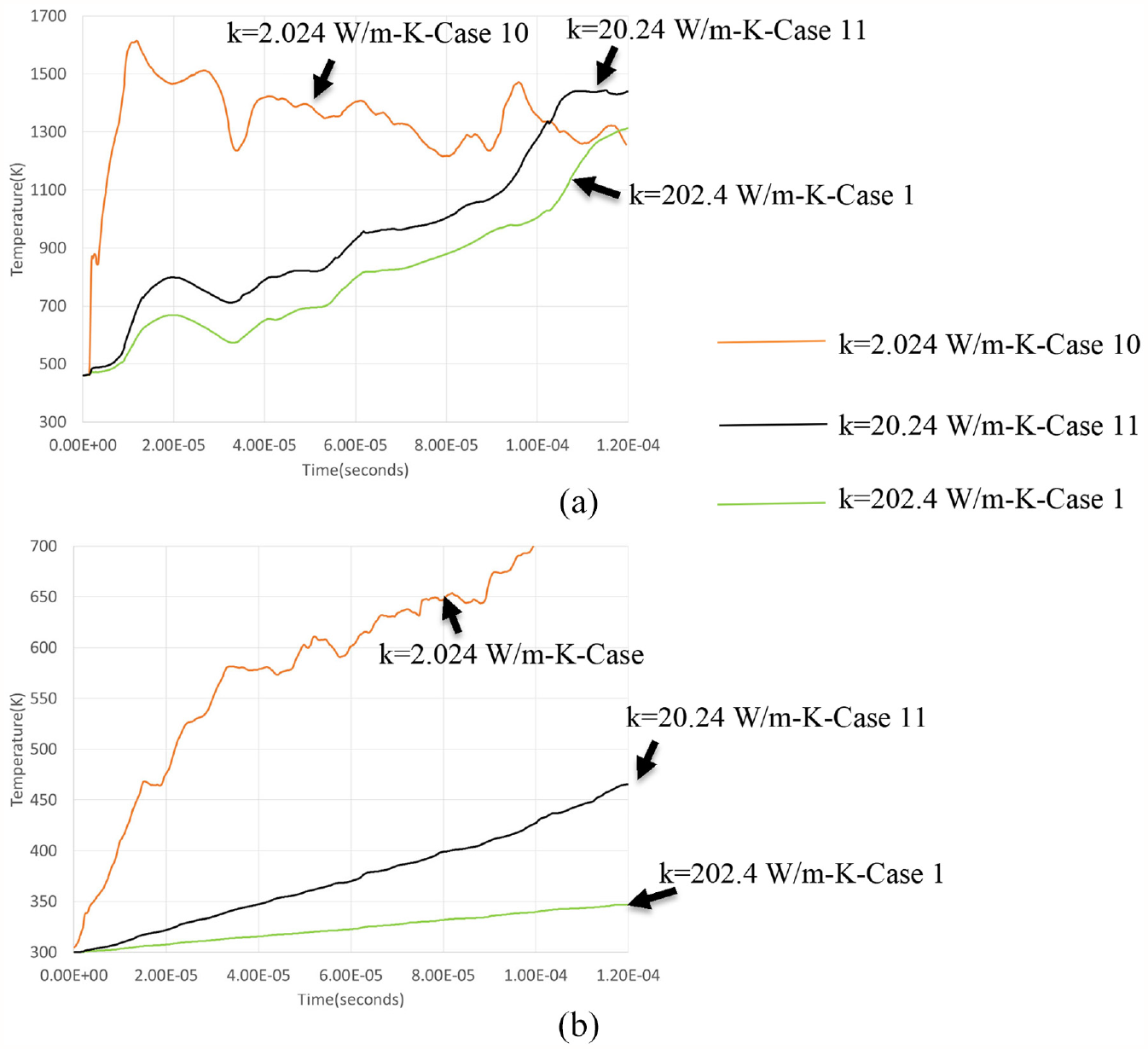
Average temperatures of the entities indicated as the thermal conductivity of the solid material is altered: (a) average temperature of particle 0 and (b) average temperature at lower flow path.

Figure 11.

Temperature contour at 5.5e–05 s for two thermal conductivity cases (Case 1 and Case 10): (a) case of k = 2.024 W/(m K) (Case 10) and (b) case of k = 202.4 W/(m K) (Case 1).

With the current method, the localized temperature field within the particles is computed so that the impact of varying the thermal conductivity of the particle material can be studied. A lower thermal conductivity provides more resistance to the heat flow and so higher temperature gradients and higher temperatures generally ensue. The higher thermal conductivity provides for faster propagation of the energy through the material, leading to more uniform particle temperatures, and generally lower temperatures. The contour plots in Figure 11 illustrate these differences. Clearly, the localized variations in the temperature conditions in the particles cannot be captured with other modeling methods. The heat flow around the particles is not uniform, indicating this modeling technique provides novel and unique capabilities so that local flow and temperature condition driven phenomena can then be studied. The numerical data presented in Figure 10 can be used to quantify the trends. The lower thermal conductivity material, when exposed to similar gas flow conditions, produces higher temperatures both at the particle surface and along the flow path surface. The oscillations in this temperature set are greater due to the greater temperature differences between the particles and the resulting local thermal effects as is evident in the contour plots in Figure 11. The temperature fields within each particle are highly dependent not only on the particle–particle contact but also on the convective heating. With the moving particles and the gas flows streaming between the particles, the high-velocity regions shift with time and position and the temperature of the gas also varies. Hence, particle interface regions exposed to the high temperature gas moving at high velocities will have higher levels of convective heating than those segments exposed to lower speed flows even on the same particle. The temperature increase at the particle surface at about 9.5e–05 s in Figure 8(a) is due to the passage of the particle through a plume of hot gas. The temperature of the flow path surface exhibits a large difference in average temperature across the thermal conductivity values with a low-conductivity average temperature 129% higher than that for the highest conductivity case as in Figure 10(b). The low-conductivity case is also more sensitive to the changes in the gas flow temperatures and the individual contacts with the particles.

The local temperature distribution within the particles that develop as a result of the gas–flow and particle–particle, and particle–flow path/obstruction interactions can be estimated using the technique described in this work, providing insight into the particle conditions that develop and the ways in which the local temperature distributions can be altered. Such local effects, evident in the contour plots, cannot be captured appropriately when the particles are not included in the computational domain.

4.5. Effect of particle specific heat

The specific heat of a material affects the thermal storage of the solid body and therefore temperature rise, much like the density, but with no change in mass of the solid body. The solid specific heat was set to a baseline and then 10 and 100 times lower in cases 1, 9, and 8. Figure 12 provides the average surface temperatures for particle 0 and for the lower flow path surface segment over time, while a general comparison of the temperature field characteristics can be gained from the temperature contours in Figure 13.

Figure 12.

Average temperatures of the entities indicated as the specific heat of the solid material is altered: (a) average temperature of particle 0 and (b) average temperature at lower flow path.

Figure 13.

Temperature contour at 1.1e–05 s for the two specific heat cases (Case 1 and Case 8): (a) case of cp = 8.71 J/(kg K) (Case 8) and (b) case of cp = 871 J/(kg K) (Case 1).

In general, solids with a higher specific heat and a greater thermal storage capacity experience lower temperature increases when compared to a system with a lower specific heat subject to the same thermal loading. The initial temperature rise is greatest for the lowest specific heat value as in Figure 12 due to the lower thermal capacity of the material for both the sample particle and the flow path. The noticeable temperature rise in a confined portion of the flow path at C and the particle 0 for the lower specific heat case in Figure 13(a) contrasts with the minimal temperature changes for the higher specific heat cases in Figure 13(b). Conduction contact heating of the flow obstruction can be observed in area B in Figure 13(a), while little noticeable heating due to particle contact is seen in Figure 13(b) with the higher specific heat value. For the lower specific heat case, the concentrated heating due to convective effects is seen by the region of yellow coloration on the upstream side of the left-most particle in the middle row and the diminishing yellow temperature regions on the upstream side of the second and third particles in that row, but now more to the sides rather than near the typical stagnation site on the second and third particles. The high speed flow moving around the first particle in that row generates two higher speed streams that impinge upon the upstream top and bottom surfaces of the downstream particles leading to the restricted regions of higher heat flow. The connections between the particle positioning, flow, and particle temperatures can be inferred from these studies. The focused and limited nature of regions of higher temperature changes is also noted from these results.

Numerical estimates of the effects of the property changes can also be gleaned from the data to correlate with the qualitative findings above. At a given time of 2.00e–05 s, the surface temperature of particle 0 is 175% higher than its initial value with the lowest specific heat value, while for the highest specific heat, the change is only 35% (Figure 12(a)). Individual alterations in the temperature can be tied to physical events. For example, the decrease in the temperature of particle 0 near 2.0e–05 s for the two higher specific heat cases is associated with particle contact with the cooler flow path wall. By about 6.0e–05 s, for the low specific heat case, particle 0 has nearly reached a steady value, close to the fluid bulk temperature, while the temperatures are still rising for the two remaining specific heat cases, but all cases appear to point to particle temperatures that approach the bulk flow temperature over time. In addition, the temperature jump after 1.0e–04 s for the lowest specific heat is due to the convective heating of the particle as it moves through a high temperature gas stream in the wake of the flow obstruction. A striking difference in the flow path temperature distribution from that with the higher specific heat can also be observed with the temperature–time slope for the low specific heat case over 14 times higher than that for the baseline, highest specific heat value.

Hence, the models allow for the capture of data and understanding the local temperatures, local flow features, and the material properties. These localized effects are apparent in the contour plots and in the discussion of results. Hence, any events driven by the local conditions including the particle motion and heating and any temperature-dependent phenomena can be better simulated using these methods if these events are of interest.

4.6. Effect of particle Young’s modulus

Young’s modulus affects the mechanical impact-based force calculations. In this study, Young’s modulus values at double and half of a baseline value are applied to the model (Cases 1, 12, 13, and 14). Figure 14 includes the temperature versus time plots for the surface average temperatures of particle 0 and the portion of the lower flow path surface while Figure 15 provides a snapshot of the temperature contours among the extreme Young’s modulus values tested.

Figure 14.

Average temperatures of the entities indicated as Young’s modulus of the solid material is altered: (a) average temperature of particle 0 and (b) average temperature at lower flow path.

Figure 15.

Temperature contour at 8.75e–05 s for two Young’s modulus cases (Case 12 and Case 14): (a) case of E = 1.00E + 10 N/m² (Case 12) and (b) case of E = 20.00E + 10 N/m² (Case 14).

The higher Young’s modulus corresponds to a higher material stiffness, a stronger contact force, a smaller contact area, and a shorter contact time, so the forces and duration of the thermal conductive heat transfer will vary with Young’s modulus value. The simulation results for the cases and conditions investigated indicate the temperatures of the particles and the flow path walls are more sensitive to changes in the density, thermal conductivity, and specific heat than to changes in Young’s modulus. Doubling and halving Young’s modulus led to less than a 1% change in the average particle 0 surface temperature through a time of 3.0e–05 s (Figure 14(a)), before contact with the flow obstruction. After this, the deviation in the temperatures is mainly due to the different location of the particles resulting from the different contact force. The larger contact force from the higher Young’s modulus leads to rebound of the particles further upstream than with the lower Young’s modulus, delaying the passage of the particles around the flow obstruction and altering the positioning of the particles in the system. The changes in the particle temperature with time after 4.0e–05 s are mainly due to the interaction of the particle and the high temperature gas stream in the wake of the flow obstruction and so the different particle positioning at a given time. The particles marked A and B in the contours in Figure 15 correspond to the same particles indicating the difference in the particle temperature and location as a result of the specific history of the contacts and gas condition exposure that each particle encounters, in this case as Young’s Modulus changes. Hence, the particle position in the system and the positioning along the particle where particle–flow feature and particle–particle/wall contact occurs governs the temperature field development in the particle.

Because the variation in Young’s modulus only affects the particle–wall particle–particle contact, the positioning of the particles and the duration of contact may vary. With the large mass of the flow path compared to the particles and only the differences in the local contact conduction, Young’s modulus changes do not have a significant impact on the flow path temperature (Figures 14(b) and 15). The contour plots and discussion clearly indicate the localized nature of the flow conditions and the thermal conditions in the system, including at the particle–flow interfaces. Hence, the modeling technique can be used to explore the sensitivity of different parameters on the local flow conditions and to provide a reasoning for why these trends and conditions occur. The technique can also be used as a means to explore methods to change the system conditions.

4.7. Effect of cohesion force parameter, β

The cohesion force parameter also affects the duration and magnitude of the interaction forces and the duration/contact area for the thermal contact between two objects. In this work, the cohesion force parameter, β, (Equation (9)) is varied from 0 to 1.0e–03 in cases 1 and 5 through 7 (Table 1), and the effect on the temperature field and particle motion is monitored. Figure 16 depicts the surface average temperature of particle 0 and the lower flow path section surface average temperatures as a function of time and Figure 17 provides a temperature contour comparison at a given time for the extreme parameters investigated.

Figure 16.

Average temperatures of the entities indicated as the cohesion force parameter is altered: (a) average temperature of particle 0 and (b) average temperature at lower flow path.

Figure 17.

Temperature contour at 5.5e–05 s for two of the cohesion parameter cases (Case 5 and Case 7): (a) case of β = 0.0E–03 (Case 5) and (b) case of β = 1.5E–03 (Case 7).

The behavior of the particle interactions is altered with the variation in the strength of the cohesion forces at work. The differences in the particle arrangement as the cohesion parameter varies can be readily observed in Figure 17 with closer packed particles and the maintenance of particle at a closer proximity to the flow path walls for the higher cohesion forces and a greater particle spread for the lower cohesion force parameter. As with the discussion of the previous parameter cases, the variation in the particle conditions is minimal until a time of about 3.0e–05 s is reached (Figure 16(a)), which corresponds to the time the particle pack impacts the obstructing plate and the particles are forced to interact with one another. The higher cohesion parameter results in more significant temperature oscillations due to the longer contact time and therefore greater conductive contact heat transfer. The temperature variation in the average particle value at the end of the time period studied is the result of the high temperature wake flow moving over the particles, a localized effect. At the flow path wall surfaces, a minimal temperature change is seen until the cohesion parameter reaches the highest value studied at 1.50e–03. At this cohesion level, the particles roll along the flow path surfaces and the heat transfer between the particles and the wall is increased as seen in Figure 16(b) and the contour plots in Figure 17. The particles rolling along a surface and the resulting flow patterns with a given particle arrangement would be difficult if not impossible to model using standard DEM-Eulerian type modeling methods. In addition, the resulting local flow and thermal effects can be modeled using the current method.

4.8. Effect of driving pressure

The higher driving pressure in the system produces higher velocities in the gases moving along the flow path. As the fluid kinetic energy is converted to pressure and thermal energy upon fluid impingement on the particle and flow path surfaces, the higher velocity results in higher pressures and temperatures, affecting both the forces acting on the particles and the heat transfer in the system. The effect of the initial tank gas pressure or driving pressure is studied with values ranging from a baseline value and double and triple this pressure (Cases 1, 15, and 16). The temperature results at particle 0 and at a portion of the flow path surface are provided in Figure 18 with representative contour plots in Figure 19.

Figure 18.

Average temperatures of the entities indicated as the driving pressure is altered: (a) average temperature of particle 0 and (b) average temperature at lower flow path.

Figure 19.

Temperature contour at 5.5e–05 s for two driving pressure cases (Case 1 and Case 15): (a) case of P = 4.0E + 07 Pa (Case 1) and (b) case of P = 1.20E + 08 Pa (Case 15).

Noticeable differences in the particle motion can be seen right as the flow reaches the particles. Not only does the higher pressure flow reach the particles slightly earlier, but since the pressure imparted by the fluid on the particles is higher, significant particle–particle impacts occur earlier as does particle impact with the flow obstruction. The differences in the particle temperatures across the initial pressure values can be plainly seen in Figure 18(a). The “stronger” incoming flow acts to oppose the rebound of the particles from the flow obstruction. In addition, the combination of the higher temperatures of the gas surrounding the particles and the faster gas velocities results in higher heat transfer to the particles. The temporal variations are strongly influenced by the temperatures of the gases moving over the surfaces, with the more abrupt changes related to the particle contacts, with both heat transfer modes having highly localized effects on a particle surface. Similarly, the higher velocities result in higher gas temperatures near the surface of the flow path and therefore higher flow path surface temperatures. The contour plots in Figure 19 indicate the same particles marked A and B and illustrate the retarded particle motion and lower particle temperatures for the lower driving pressure. This set of models demonstrates how the local temperatures and gas conditions can impact the particle motion and heating and how the current modeling method is useful for capturing these effects. The effects of specific particle–particle/other surface and particle–flow interactions can be gleaned from the simulations and used to predict additional phenomena, information that may not be obtained if particles/objects were not directly in the flow.

4.9. Effect of radiation properties

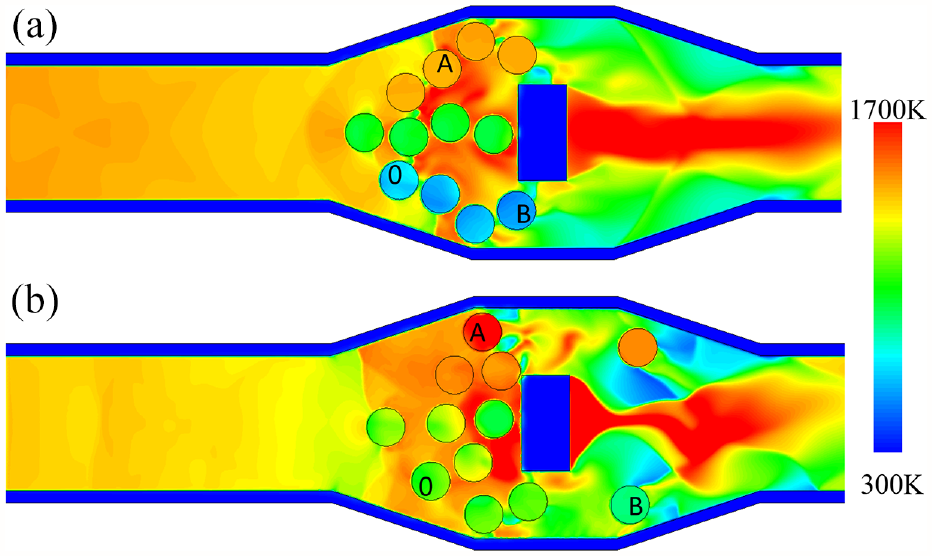
Finally, the radiation exchange between particle surfaces and particle surfaces and the surfaces of other solid bodies is incorporated into the simulation. To amplify the radiative heat exchange in the time period studied, the initial particle temperatures are increased. The gray body assumption is applied with emissivity values of 0 and 1.0 in cases 17 and 18. Examination of the results of the simulations, including the average particle 0 surface temperature and the average temperature over the section of the lower flow path in Figure 20 and the contours of the temperature fields for these two cases in Figure 21, provides information on the sensitivity of the flow and particle conditions to the inclusion of the radiation effects.

Figure 20.

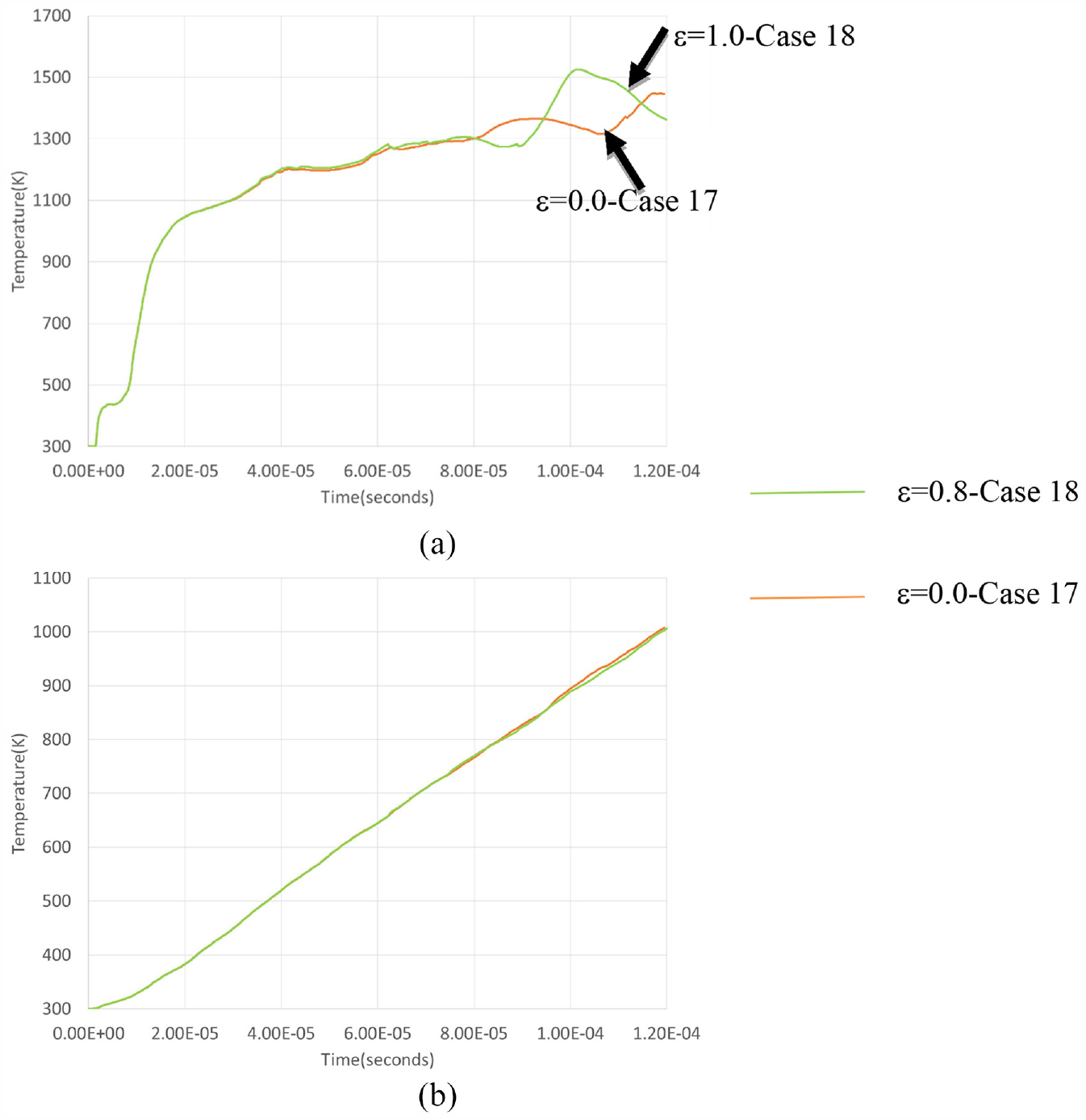
Average temperatures of the entities indicated radiation ε is altered, elevated temperature: (a) average temperature of particle 0 and (b) average temperature at lower flow path.

Figure 21.

Temperature contour at 8.5e–05 s with and without radiation, elevated temperature (Case 17 and Case 18): (a) case of ε = 0.0 (Case 17) and (b) case of ε = 1.0 (Case 18).

Initially, the cases with and without the radiation exchange show little difference, indicating the convective effects dominate and that sustained radiative heat transfer is needed to produce a noticeable temperature change due to the radiation effects. Just after 8.0e–05 s, the temperature decrease at particle 0 for Case 18 as seen in Figure 20(a) is due to the radiation exchange with the cooler flow path surface. The slight differences in the particle positioning and temperatures that occur for the different cases can influence the subsequent temperatures (Figure 21) with the radiation Case 18 particle moving through the high temperature flow stream earlier than the non-radiation Case 17, causing the temperature rise observed after 9.0e–05 s. However, the radiation exchange with the cool wall results in the decrease in the particle temperature seen after 1.00e–04 s. With the large surface area of the flow path and the limited frequency of the particle contact or proximity, changes in the radiation effects for this system have little impact on the temperatures of the flow path (Figures 20(b) and 21). The fundamental effects behind the trends in the particle temperature and wall temperature can be clearly captured through the use of the new modeling technique. With the discretized particles, the locally varying temperatures and the geometry itself can be used in formulating the radiative energy exchange. Such surface–surface radiation exchange is not possible if the particles are not discretized in the system. In addition, if desired, radiation exchange with the gases could be included. These details could not be captured in standard modeling methods.

5. Conclusion and future work

Under conditions of larger, interacting particles carried through a flow path by gas flow, the local flow and temperature conditions are highly time and location dependent. The flow moving over one particle has evolved as a result of the motion and positioning of the neighboring particles and the open flow paths between the particles. Standard correlations for drag and heat transfer coefficients may not be valid under such conditions and the temperatures, pressures, and velocity fields typically vary significantly around the particle–flow interface as demonstrated in the examples presented in this work. Such conditions are difficult to capture in a numerical model if the particles are not discretized within the computational domain such as in the standard DEM-Lagrangian-Eulerian modeling method. When local temperature-dependent phenomena including material property changes, chemical reactions, or phase change are of interest, the capability to capture these local time, space, and system geometry-dependent fields is critical to simulating these phenomena and analyzing, understanding, and identifying the underlying causes for such items as reaction rates, species distribution, or phase generation that develop. This work has strongly demonstrated the ability of the modeling method discussed to provide the information necessary to analyze higher particle size and concentration conditions and particularly the cases where local temperature variations, pressure levels, and/or velocity gradients at particle–flow interfaces or even within the particle drive the processes of interest.

The modeling method developed provides information that is difficult to obtain through experimental techniques. Experimentally capturing the motion of each particle, the temperature distribution within each particle, the details of the flow field that results, the forces due to the flow and mechanical interactions, the thermal contact effects, radiation, and conjugate heat transfer, and an understanding of the relative contributions of the forces and heat flow respectively would be nearly impossible to obtain through physical testing. The numerical models then can be used to gain insight into the operation of these particle-laden flow systems that may not be attainable through other means.

Based on this work, a number of future work paths can be pursued. Comparisons of the bulk particle motion for a given geometry, particle, and flow condition set to the modeling method results can be attempted, recognizing that not all data captured in the model can be replicated experimentally. Individual components of the modeling method have already been compared to results for simulations of the mechanical and thermal contact events, respectively. The method can be applied to study local temperature-dependent processes such as chemical reactions, solidification, melting, sublimation, temperature-varying adhesion forces, and temperature-varying properties. The large computational requirements for directly modeling the particles and other moving solids in the flow are recognized. Means of using these simulations to train machine learning algorithms so that spatial variation in the flow and thermal effects at the fluid–solid interface can be gleaned could be investigated. These algorithms might then be used to reduce the computational burden while expanding the phenomena that can be addressed. Hence, with this modeling method, the range of conditions and phenomena that can be studied can be expanded and the understanding of the particle-laden flow can be improved.

Footnotes

Appendix

Appendix 1

Notation

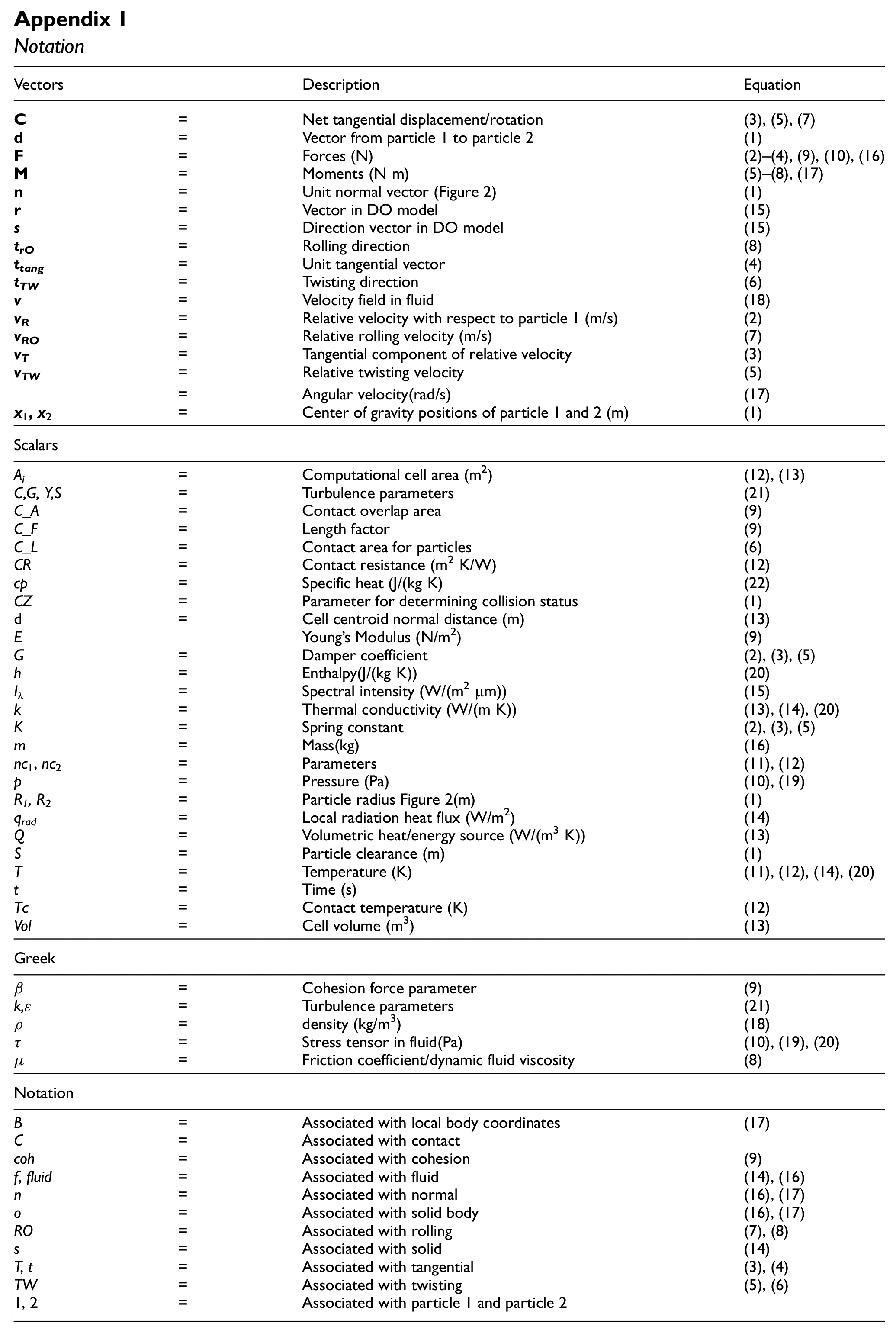
Vectors		Description	Equation
C	=	Net tangential displacement/rotation	(3), (5), (7)
d	=	Vector from particle 1 to particle 2	(1)
F	=	Forces (N)	(2)–(4), (9), (10), (16)
M	=	Moments (N m)	(5)–(8), (17)
n	=	Unit normal vector (Figure 2)	(1)
r	=	Vector in DO model	(15)
s	=	Direction vector in DO model	(15)
t_rO	=	Rolling direction	(8)
t_tang	=	Unit tangential vector	(4)
t_TW	=	Twisting direction	(6)
v	=	Velocity field in fluid	(18)
v_R	=	Relative velocity with respect to particle 1 (m/s)	(2)
v_RO	=	Relative rolling velocity (m/s)	(7)
v_T	=	Tangential component of relative velocity	(3)
v_TW	=	Relative twisting velocity	(5)
Ω	=	Angular velocity(rad/s)	(17)
x ₁, x ₂	=	Center of gravity positions of particle 1 and 2 (m)	(1)
Scalars
A_i	=	Computational cell area (m²)	(12), (13)
C,G, Y,S	=	Turbulence parameters	(21)
C_A	=	Contact overlap area	(9)
C_F	=	Length factor	(9)
C_L	=	Contact area for particles	(6)
CR	=	Contact resistance (m² K/W)	(12)
cp	=	Specific heat (J/(kg K)	(22)
CZ	=	Parameter for determining collision status	(1)
d	=	Cell centroid normal distance (m)	(13)
E		Young’s Modulus (N/m²)	(9)
G	=	Damper coefficient	(2), (3), (5)
h	=	Enthalpy(J/(kg K))	(20)
I_λ	=	Spectral intensity (W/(m² µm))	(15)
k	=	Thermal conductivity (W/(m K))	(13), (14), (20)
K	=	Spring constant	(2), (3), (5)
m	=	Mass(kg)	(16)
nc ₁, nc₂	=	Parameters	(11), (12)
p	=	Pressure (Pa)	(10), (19)
R₁, R₂	=	Particle radius Figure 2(m)	(1)
q_rad	=	Local radiation heat flux (W/m²)	(14)
$Q$	=	Volumetric heat/energy source (W/(m³ K))	(13)
S	=	Particle clearance (m)	(1)
T	=	Temperature (K)	(11), (12), (14), (20)
t	=	Time (s)
Tc	=	Contact temperature (K)	(12)
Vol	=	Cell volume (m³)	(13)
Greek
β	=	Cohesion force parameter	(9)
k,ε	=	Turbulence parameters	(21)
ρ	=	density (kg/m³)	(18)
τ	=	Stress tensor in fluid(Pa)	(10), (19), (20)
µ	=	Friction coefficient/dynamic fluid viscosity	(8)
Notation
B	=	Associated with local body coordinates	(17)
C	=	Associated with contact
coh	=	Associated with cohesion	(9)
f, fluid	=	Associated with fluid	(14), (16)
n	=	Associated with normal	(16), (17)
o	=	Associated with solid body	(16), (17)
RO	=	Associated with rolling	(7), (8)
s	=	Associated with solid	(14)
T, t	=	Associated with tangential	(3), (4)
TW	=	Associated with twisting	(5), (6)
1, 2	=	Associated with particle 1 and particle 2

Funding

This work was supported by a US Army Armament Graduate School Faculty Research Award. This work was supported in part by a grant of computer time from the DoD High Performance Computing Modernization Program at ARL, AFRL, and ERDC.

ORCID iD

Laurie A Florio

Author biography

Laurie A Florio is a Mechanical Engineer within the US Army DEVCOM Armaments Center at Picatinny Arsenal, NJ and is an Assistant Professor at the US Army Armament Graduate School at Picatinny Arsenal.

References

Florio

LA.

Computation of fluid–particle interactions with high-speed compressible flows and multiple particles with deformation, plasticity, and collisions. Powder Technol 2014; 268: 19–37.

Florio

LA.

Dynamic coupling of fluid and structural mechanics for simulating particle motion and interaction in high speed compressible gas particle laden flow. J Fluid Struct 2015; 54: 171–201.

Florio

LA.

Direct modeling of coupled compressible flow and macroscopic particle spread and particle ejection. Meccanica 2015; 50: 2257–2291.

Florio

LA.

Estimation of particle impact based erosion using a coupled direct particle—compressible gas computational fluid dynamics model. Powder Technol 2017; 305: 625–651.

Florio

LA.

Development of novel heat conduction interaction model for solid body thermal contact in CFD based particle flow simulations. Chem Eng Sci 2018; 192: 448–466.

Florio

LA.

Conduction, convection, and radiation thermal exchange with discretized fixed, contacting particles in a high speed compressible flow. Int J Heat Mass Tran 2019; 133: 137–153.

Cundall

Strack

ODL

. Discrete numerical model for granular assemblies. Geotechnique 1979; 29: 47–65.

Di Renzo

Di Maio

. Comparison of contact-force models for the simulation of collisions in DEM-based granular flow codes. Chem Eng Sci 2004; 59: 525–541.

Tsuji

Tanaka

Ishida

Lagrangian numerical simulation of plug flow of cohesionless particles in a horizontal pipe. Powder Technol 1992; 71: 239–250.

10.

Chen

Zhong

Zhou

, et al. CFD–DEM simulation of particle transport and deposition in pulmonary airway. Powder Technol 2012; 228: 309–318.

11.

Grof

Cook

Lawrence

, et al. The interaction between small clusters of cohesive particles and laminar flow: coupled DEM/CFD approach. J Petrol Sci Eng 2009; 66: 24–32.

12.

Vargas

McCarthy

JJ.

Conductivity of granular media with stagnant interstitial fluids via thermal particle dynamics simulation. Int J Heat Mass Tran 2002; 45: 4847–4856.

13.

Liu

Simulation of effect of internals on particulate mixing and heat transfer in downer reactor using discrete element method. Powder Technol 2016; 297: 89–105.

14.

Yang

Zhou

AB.

Particle scale studies of heat transfer in a moving bed. Powder Technol 2015; 281: 99–111.

15.

Cheng

Zhang

Numerical investigation on the transient ignition behavior using CFD-DEM approach. Combust Sci Technol 2014; 186: 1115–1137.

16.

Oschmann

Schiemann

Kruggel-Emden

Development and verification of a resolved 3D inner particle heat transfer model for the Discrete Element Method (DEM). Powder Technol 2016; 291: 392–407.

17.

Liu

Gui

Yang

, et al. A DEM-embedded finite element method for simulation of the transient heat conduction process in the pebble bed. Powder Technol 2021; 377: 607–620.

18.

Liang

A series solution based formulation for discrete thermal element method of granular materials. Granul Matter. Epub ahead of print 14 January 2021. DOI: 10.1007/s10035-020-01074-2.

19.

Joulin

Xiang

Latham

, et al. Capturing heat transfer for complex-shaped multibody contact problems, a new FDEM approach. Comput Part Mech 2020; 7: 919–934.

20.

Adepu

Chen

Jiao

, et al. Wall to particle bed contact conduction heat transfer in a rotary drum using DEM. Comput Part Mech 2021; 8: 589–599.

21.

Dai

Thermal conduction in granular media: from interface, topology to effective property. PhD Thesis, The University of Sydney, Sydney, NSW, Australia, 2019.

22.

Bea

Mancardo Viotti

Carusela

, et al. Assessment, improvement, and comparison of different computational tools used for the simulation of heat transport in nanostructures. Simulation. Epub ahead of print 27 April 2021. DOI: 10.1177/00375497211009611.

23.

Wang

Effect of particle clusters on mass transfer between gas and particles in gas-solid flows. Powder Technol 2017; 319: 221–227.

24.

Wang

Sierakowski

Prosperetti

Fully-resolved simulation of particulate flows with particles fluid heat transfer. J Comput Phys 2017; 350: 638–656.

25.

Das

Deen

Kuipers

JAM

. A DNS study of flow and heat transfer through slender fixed-bed reactors randomly packed with spherical particles. Chem Eng Sci 2017; 160: 1–19.

26.

Tafti

DK.

Heat transfer in an assembly of ellipsoidal particles at low to moderate Reynolds numbers. Int J Heat Mass Tran 2017; 114: 324–336.

27.

Johnson

Tezduyar

TE.

Advanced mesh generation and update methods for 3D flow simulations. J Comput Mech 1999; 23: 130–143.

28.

Glowinski

Pan

Hesla

, et al. A fictitious domain approach to the direct numerical simulation of incompressible viscous flow past moving rigid bodies: application to particulate flow. J Comput Phys 2001; 169: 363–426.

29.

Florio

LA.

Numerical investigation of particle trapping in various groove configurations in straight and bent flow channels. Simulation 2020; 96: 679–699.

30.

Balachandar

Moore

Akiki

, et al. Toward particle-resolved accuracy in Euler–Lagrange simulations of multiphase flow using machine learning and pairwise interaction extended point-particle (PIEP) approximation. Theor Comp Fluid Dyn 2020; 34: 401–428.

31.

Ganti

Khare

Data-driven surrogate modeling of multiphase flows using machine learning techniques. Comput Fluids 2020; 211: 104626.

32.

Matuttis

H-G

Chen

Understanding the discrete element method. Singapore: Wiley, 2014.

33.

Marshall

Adhesive particle flow. New York: Cambridge University Press, 2014.

34.

Chui

Raithby

GD.

Computation of radiant heat transfer on a nonorthogonal mesh using the finite-volume method. Numer Heat Tr B: Fund 1993; 23: 269–288.

35.

Shames

IH.

Engineering mechanics: dynamics. New York: Prentice Hall, 1996.

36.

Ickes

BP.

A new method for performing digital control system attitude computations using quaternions. AIAA J 1970; 8: 13–17.

37.

White

FM.

Viscous fluid flow. New York: McGraw Hill, 1991.

38.

Shih

T-H

Liou

Shabbir

, et al. A new k-ϵ eddy viscosity model for high Reynolds number turbulent flows. Comput Fluids 1995; 24: 227–238.

39.

McBride

Zehe

Gordon

. NASA Glenn coefficients for calculating thermodynamic properties of individual species. National Aeronautics and Space Administration (NASA) technical report TP-2002-211556, September 2002. Washington, DC.