
Abstract
Emergency Medical Service (EMS) managers continuously strive to improve the coverage performance, i.e., the percentage of calls responded to within a specific target time, to save lives in case of life-threatening emergencies. This goal can be achieved by dynamically adjusting the location of rescue teams during a day in response to some temporal or geographical fluctuations such as demand patterns, traffic conditions, or the number of teams on duty. This relocation is known as the multi-period redeployment problem. In this study, we propose a discrete simulation-based optimization model to adress the multi-period redeployment problem in the French EMS of the Val-de-Marne department (France), named SAMU 94. The proposed model uses an iterative method that combines the use of a mathematical model to find the optimal locations of rescue teams with the use of the SAMU 94 simulation model implemented in Arena software, to evaluate the busy fraction parameters required to solve the mathematical model. The model performance was compared with that of the simulation-based optimization software, OptQuest. The experimental results demonstrated that the iterative method could produce solutions with better coverage performance, 20 times faster than OptQuest.
Keywords
1. Introduction
In France, the emergency medical service (EMS) is known as SAMU, a French acronym of “Urgent Medical Aid Service.” The SAMU provides phone support and pre-hospital care to patients under emergency conditions. Pre-hospital care consists of assessing and stabilizing the patient at the incident scene before his or her transport to the appropriate care facility. The basic procedure of a SAMU rescue is as follows: Central operations are triggered whenever a rescue call is received in the reception and regulation (R&R) center. Staff in the R&R center provides phone support and decides whether the rescue event is urgent enough to dispatch a rescue team to the scene. The dispatch of a rescue team triggers the external operations. The rescue team provides first aid to the patient at the scene and transports the patient to a hospital when necessary before returning to its home base. A home base is a fixed station where a rescue team is placed between rescues.
The main objective of the SAMU system is to save lives and reduce the disability of the victims. In life-threatening emergencies, several authors observed the association between high survival rate or reduced disability and low response time, defined as the period between receiving a call and the first arrival of a rescue team at the incident scene. For example, for cardiac arrest victims, every minute without life-saving cardiopulmonary resuscitation (CPR) and defibrillation reduces the chance of survival by 7%–10%. 1 For acute myocardial infarction, the risk of 1-year mortality is increased by 7.5% for each 30-min delay in treatment of patients. 2 Therefore, having high coverage, i.e., the percentage of calls for which response time does not exceed a specific target time, is a commonly expressed objective for the SAMU managers.
To ensure high coverage of the service area, rescue teams need to be located effectively. Furthermore, considering that emergency calls and traffic conditions change dynamically due to the population’s daily activities (e.g. work, home, shopping), the assignment of rescue teams to bases should be adjusted to cover these changing conditions adequately. This problem is known as multi-period redeployment.
This study addresses the problem of multi-period redeployment, which aims to improve the coverage performance of the SAMU system in the department of Val-de-Marne (southeast of Paris, France), called SAMU 94. For this purpose, we use the discrete simulation-based optimization (DSBO) approach to find the optimal base locations for different periods on weekdays/weekends. DSBO combines discrete event simulation (DES) models and optimization techniques to search for high-quality solutions. DES mimics the stochastic behavior of complex systems and accurately assesses their performance without the need of simplifying assumptions required when using other types of analytical models, such as linear programming and queuing models. 3 It is a powerful decision-support tool that evaluates the impact of several changes in decision variables (i.e. scenarios) over different key performance indicators (KPIs).4,5 However, when the number of decision variables is large, running and comparing all possible combinations of scenarios is very expensive and time-consuming. DSBO uses optimization techniques to find the best values of the decision variables under simplifying assumptions. The obtained solution quality is then measured more realistically and refined using the DES model. 6 Many researchers agree that DSBO outperforms analytic models for investigating complex stochastic systems. 7
In the literature, many review papers describe the theory and applications of DSBO,8–10 According to Wang and Shi 9 and Chen et al., 11 a DSBO problem can be formulated as follows:

such that

Equation (1) represents the objective function where θ can be one or several decision variables, Θ is the feasible region, ω is the randomness of the DES model, and L(θ, ω) is the performance indicator value obtained from several replications of the DES model.
In this work, we propose a DSBO approach consistent with the characteristics of the multi-period redeployment problem of the SAMU 94 system, i.e., large, finite, and discrete feasible solution region Θ. This approach is an iterative method that combines DES and mathematical modeling to find the optimal locations of rescue teams. DES is used to approximate the busy fraction (i.e., the probability that a rescue team is busy) used to solve the mathematical model. DES also evaluates the coverage performance of the location solution obtained from the mathematical model. The results of this approach are compared with those obtained with the optimization simulation software OptQuest that uses metaheuristics to find the optimal values of input location variables.
The main contributions of this paper can be summarized as follows:
We provided SAMU managers with a useful decision-making tool that dynamically adjusts the location of rescue teams during a day in response to some temporal or geographical fluctuations.
Our study contributes to reducing the lack of DSBO models for multi-period relocation problems that consider variations in daily demand pattern, or travel times, or number of available rescue teams in EMS systems and provide valuable insights into the iterative method and its application to solve multi-period redeployment problems.
We demonstrated that when the solution region is large, the proposed iterative method can be an efficient tool that outperforms OptQuest by providing high-quality solutions in a shorter time.
The remainder of this paper is organized as follows. Section 2 reviews the literature about the combination of simulation with mathematical models in EMS and OptQuest in Operations Management. In section 3, we describe the SAMU 94 system and the essential elements of the DES model. Section 4 describes the mathematical model of the SAMU 94 and the iterative method. The formulation of OptQuest simulation optimization model of the SAMU 94 is presented in section 5. Section 6 compares the results obtained from the two approaches regarding computational times and coverage performance. Finally, section 7 provides conclusions and presents some directions for future research.
2. Literature review
There is extensive literature on solving ambulance location and relocation problems using mathematical programming. Ambulance location refers to determining the number and fixed location of rescue teams required to maximize the coverage performance statically, i.e., the location of each rescue team remains unchanged over the planning horizon. Ambulance relocation refers to changing rescue teams’ location over the planning horizon in response to the evolution of the EMS system condition following the change in demand pattern (multi-period redeployment) or the allocation/release of a rescue team (dynamic redeployment).
Two early deterministic models were proposed to solve the static location problem: Toregas et al. 13 formulated the location set covering problem (LSCP) that seeks to minimize the number of vehicles needed to cover the demand within a given target distance (time). Church and ReVelle 14 developed the maximal covering location problem (MCLP) that maximizes the coverage within a given target distance (time), using a limited number of vehicles. These basic models are unrealistic as they ignore the possible unavailability of rescue teams to answer a call. Thus, many models have been proposed in the literature to provide a more robust location plan. Daskin and Stern, 15 Hogan and ReVelle, 16 and Gendreau et al. 17 proposed deterministic models with multiple coverage that seeks to maximize the covered demand using more than one vehicle. Daskin 18 proposed a probabilistic model, called MEXCLP (Maximum Expected Covering Location Problem), which explicitly considers the probability that vehicles may become unavailable, named busy fraction, and seeks to maximize the expected covered demand, expressed as a function of the busy fraction. Repede and Bernardo 19 developed one of the first multi-period redeployment models, which is an extension of the MEXCLP that seeks to maximize the expected coverage while considering changes in the number of vehicles and demand pattern. Other multi-period redeployment models have been proposed to include special characteristics such as time-dependent travel times, 20 workload restrictions for personnel, 21 start-up and relocation costs. 22 For more details on the use of deterministic and probabilistic mathematical models to solve ambulance location problem, we refer the reader to the recent comprehensive reviews by Aringhieri et al. 23 and Bélanger et al. 24
The mathematical programming approach mentioned above has also largely been used in EMS literature in combination with DES. This simple combined approach sequentially uses a mathematical programming model to find an optimal location/relocation solution and then uses simulation to assess the resulting deployment/redeployment plan in a more realistic manner. Several studies have considered this approach to solve the static location problem, using deterministic models,25,26 deterministic models with multiple coverage, 27 and probabilistic models.28,29 This approach allowed to improve several EMS systems’ performance. However, surprisingly few studies have considered this approach to solve the ambulance relocation problem.19,30
The first attempt to combine mathematical models and simulation embed in an iterative procedure within the field of EMS location problem can be attributed to the study by Lee et al. 31 The authors addressed the static air ambulance location problem in Korea by developing a mathematical model to find the optimal solution for given helicopters’ busy fraction estimates. Using the obtained location solution, they used simulation to improve busy fraction estimates, which are subsequently used in the mathematical model to find an updated location solution. This iterative process continues until the location solution converges. Similarly, Bélanger et al. 32 developed an iterative approach that combines a mathematical model and DES to locate available ambulances and determine their dispatching policy. The static mathematical model is used to obtain the initial ambulance locations and dispatching lists. Then, the DES model is configured according to this initial solution to update busy fraction estimates, which are used in the mathematical model to find an updated location solution and dispatching lists. The algorithm is repeated until the convergence criterion is met. Aringhieri et al. 33 proposed an iterative greedy procedure to optimally locate ambulances in the urban area of Milano (Italy). The procedure uses a deterministic mathematical model to provide the initial location solution, which represents a lower bound of the number of ambulances needed to provide appropriate coverage under the deterministic assumption. The initial solution is assessed using agent-based simulation, which determines the ambulance with the highest utilization and adds a new ambulance in the same base to decrease the highest utilization. The iterative procedure ends when all available EMS ambulances are located.
Such iterative methods seem to be a promising approach to handle stochastic aspects in EMS location/relocation problems and to solve them efficiently. However, as mentioned in the study by Aringhieri et al., 33 the field is still relatively unexplored and requires further research to gain more insights into its capabilities. Hence, we propose an iterative method that uses mathematical modeling to improve the coverage performance of the SAMU 94 system. This model contributes to existing EMS literature by providing valuable insights into the iterative method and its application to solve multi-period redeployment problems, which is currently lacking to the authors’ best knowledge.
To assess and compare the iterative method performance, we used OptQuest for Arena. OptQuest is a commercial tool that combines several metaheuristics such as scatter search, tabu search, and neural networks into a single search routine. 34 OptQuest is widely used in recent literature to improve the performance of various complex systems. In the production management area, Melouk et al. 35 used OptQuest to obtain significant cost savings in a steel manufacturing facility with adjustments to work-in-process inventory levels. Neeraj et al. 36 used OptQuest for Arena to find the bottlenecks and achieve optimal productivity and better use of resources in an aluminum brake brackets factory. In the study by Yang et al., 37 OptQuest was used to search for the best storage area size to maximize the service level in a fishing net manufacturing system.
In the inventory management area, Sadeghi et al. 38 used OptQuest to improve total cost, including shortage cost, inventory holding cost, and ordering cost, by optimizing the values of replenishment parameters in a three-echelon supply chain system of a blood sugar strip manufacturer. Afshar-Bakeshloo et al. 39 developed a simulation-based optimization method combining OptQuest, experimental design, variance analysis, and response surface methodology to control the inventory by considering three objectives of cost, environment, and customer’ satisfaction.
In the healthcare management area, Ghanes et al. 40 developed an OptQuest model to optimize the human resource staffing levels of real-life emergency department in an urban French hospital. Chraibi et al. 41 used OptQuest to find the best operating theater layout that minimizes the traveling costs for staff and patients. Zeinali et al. 42 used OptQuest to find the near-optimal number of emergency department resources (receptionists, nurses, residents, and beds) to reduce patients’ total average waiting times, with consideration of budget and capacity constraints. Chen et al. 43 used OptQuest to improve patient referral mechanisms between two hospitals. The objective of their study was to optimize the number of referral outpatients to minimize the average waiting time of patients or to maximize the revenues of both case hospitals. Niessner et al. 44 used OptQuest to address the dynamic staff reallocation problem at advanced medical posts built to treat and stabilize patients in case of mass casualty incidents. Azcarate et al. 45 proposed an OptQuest model to obtain optimal discharge policies in an intensive care unit to optimize two conflicting objective functions: minimizing patient rejection due to full occupancy and the length of stay reduction.
Therefore, OptQuest has demonstrated the power to analyze complex systems and identify potential improvements in an extensive range of practical applications. We thus selected OptQuest for Arena to address our multi-period redeployment problem of the SAMU 94 system and to compare its relocation solution to those of the iterative approach.
3. The SAMU 94 system
3.1. System description
The SAMU 94 is the French EMS responsible for providing a 24 h pre-hospital care service for the Val-de-Marne department. The Val de Marne is a small department of 245 km2, located in the southeast of Paris. When an emergency call is received by the SAMU 94, it is first processed by an operator in the R&R center. Operators are responsible for answering calls, identifying inappropriate calls, and creating a medical file. When the call is a medical request, the operator redirects the call to a regulator. The regulator is a medical doctor who determines whether the call is urgent enough to send a rescue team. Suppose a rescue team has to be sent, the regulator assigns a priority to the rescue based on its severity (priority 1 for life-threatening emergencies and priority 2 otherwise) and dispatches the closest available unit (either available at its base or returning from a previous rescue). If the rescue team is at the base, it prepares the rescue by retrieving the necessary equipment and rushing to the ambulance. The rescue team then departs for the incident scene. After the stabilization of the patient at the scene, the ambulance typically transports the patient to the appropriate destination hospital. Sometimes, the patient may need diagnostic or therapeutic radiography (DTR) such as MRI or X-ray. If the destination hospital is not well-equipped or has wait times that are too long, the patient is first taken to a medical service where the DTR is performed before moving to the hospital. Once at the destination hospital, the patient is handed over to the hospital staff, and the rescue team returns to its base. If transport to the destination hospital is not required, the rescue team goes back from the scene to its base. As soon as the rescue team begins traveling to its base, it is considered available to respond to a new emergency call. Figure 1 shows the SAMU 94 rescue process.
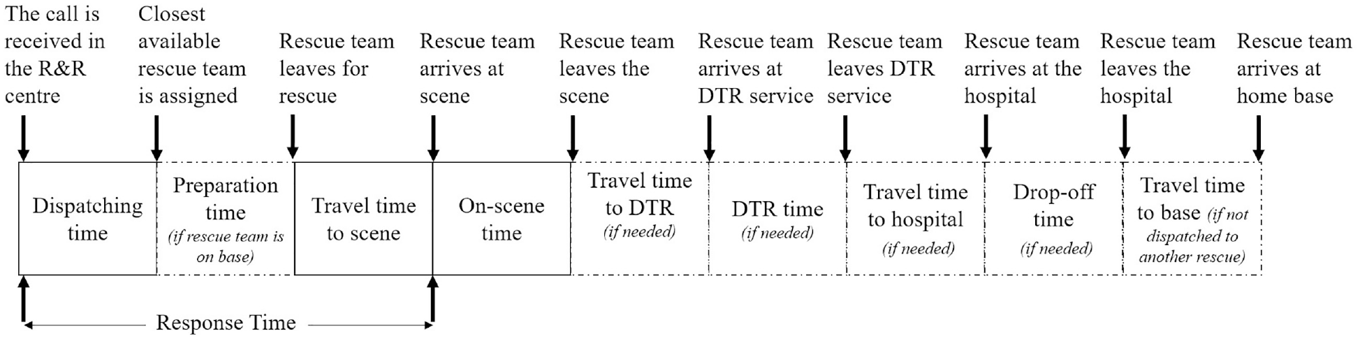
SAMU 94 rescue process.
Presently, all rescue teams are located in one central base (Henri-Mondor Hospital (HM)) and one auxiliary base (Villeneuve-Saint-Georges Hospital (VSG)). Table 1 summarizes the current number of scheduled rescue teams at each base by day of the week and time of the day.
SAMU 94–scheduled rescue teams at each base.
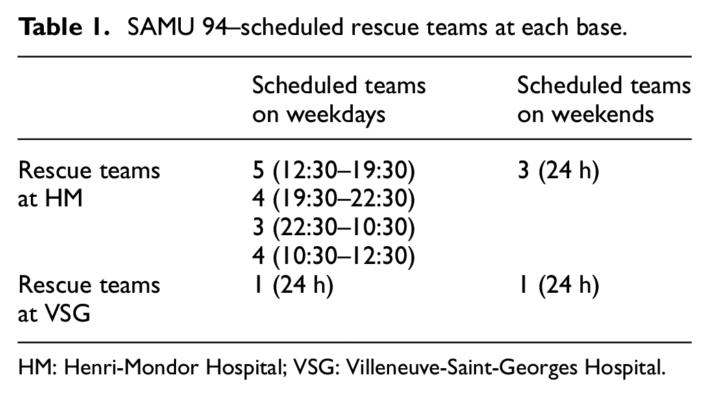
HM: Henri-Mondor Hospital; VSG: Villeneuve-Saint-Georges Hospital.
3.2. DES model
The key inputs required to build the DES model are summarized in Table 2. To estimate these inputs properly, the data from the SAMU 94 were collected for 15 months of operations. Based on these data, the arrival process of calls was fitted with a non-homogeneous Poisson process with a time-varying rate as the obtained p-values of Kolmogorov–Smirnov and Chi-square goodness-of-fit tests were greater than 0.05. 46 The processing times (i.e., dispatching time, preparation time, on-scene time, DTR time, and drop-off time) were fitted with empirical distributions because goodness-of-fit tests for theoretical distributions provided low p-values. 47 Finally, particular attention was given to model travel times between bases, scenes, DTR services, and hospitals, as this is a critical component to assess redeployment plans adequately. We first estimated the average travel time along roads of the Val de Marne department at various periods, using the global positioning system (GPS) traces of the SAMU-94 ambulances. The Val de Marne department has been broken down into IRIS (i.e. French acronym of “aggregated units for statistical information”), which are nodes of approximately 2000 residents. The aggregation of calls into a node structure is a common trade-off in the simulation of EMS systems to reduce computational times. 12 We used 527 IRIS in the Val de Marne department to locate calls and roads’ average travel times to pre-compute the shortest path from every possible origin IRIS to every possible destination IRIS, for various periods that represent different degrees of traffic congestion on weekdays (6:00–10:00, 10:00–15:00, 15:00–21:00, and 21:00–6:00) and weekends (12:00–21:00 and 21:00–12:00). A regression factor estimated at 0.937 was used to decrease travel times for priority 1 rescues to capture the fact that vehicles are allowed to travel at all possible speeds for this type of rescues.
Input data required to run the DES model.
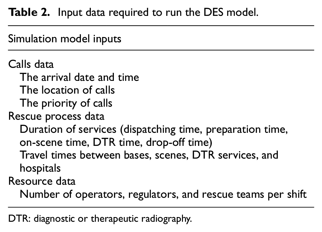
DTR: diagnostic or therapeutic radiography.
Based on the previously described rescue process and data, the DES model was summarized into a conceptual model (Figure 2) and then computerized model using Arena software. We ran the DES model for 15 months and 20 replicated times, resulting in a total run time of 35 min. The system was initialized between replications to calculate the 95% confidence intervals of outcome variables, including coverage for different priorities/target times. The SAMU 94 managers have validated the DES model. They confirmed that the model’s conception and outputs are reliable compared to real-world system behavior. We also performed event validity and historical data validation by ensuring that the simulated number of calls and coverage within different time threshold (i.e., 10, 15, and 20 min) for each priority are close enough to the observed distributions. Results are depicted in Figure 3. The Figure showed that the difference between the historical and simulated values does not exceed 6% for the number of calls and 8.9% for the coverage performance. A more detailed description of the system process, data collection, DES model design, implementation, and validation is provided by the authors in a previous study. 46

SAMU 94 simulation conceptual model.
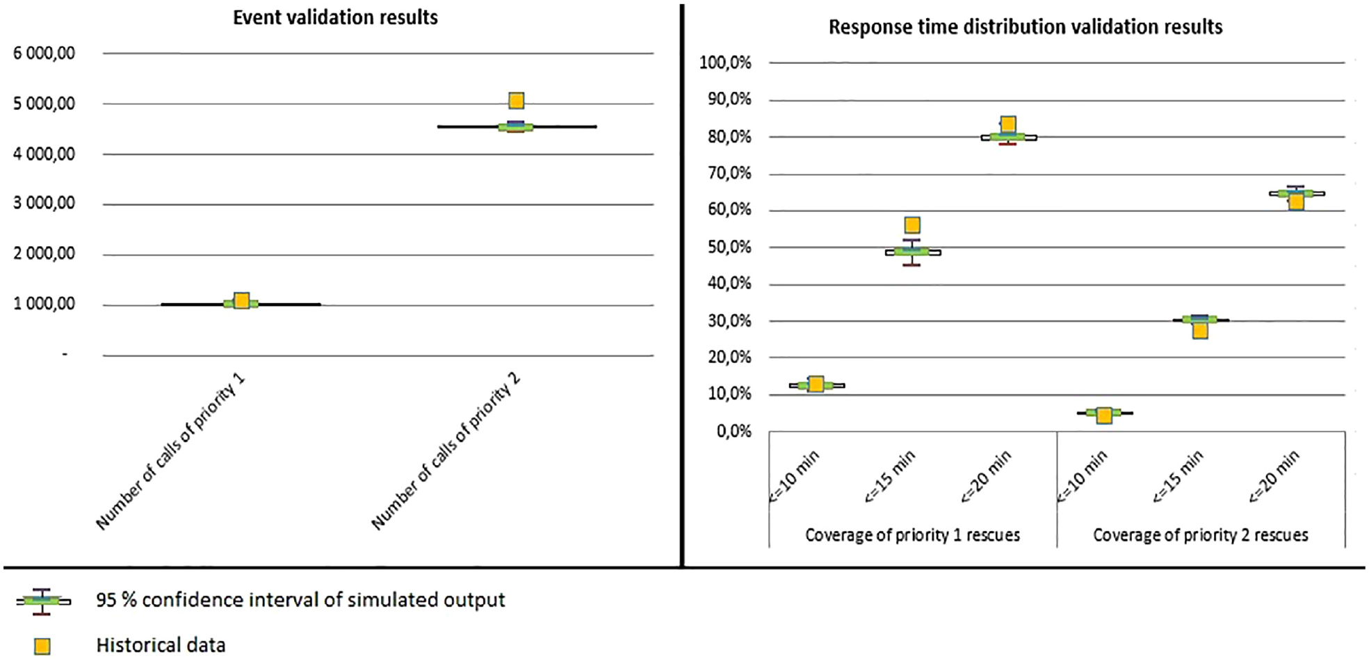
Event validity and historical data validation.
4. The iterative method for the SAMU 94 multi-period redeployment problem
4.1. The mathematical multi-period model
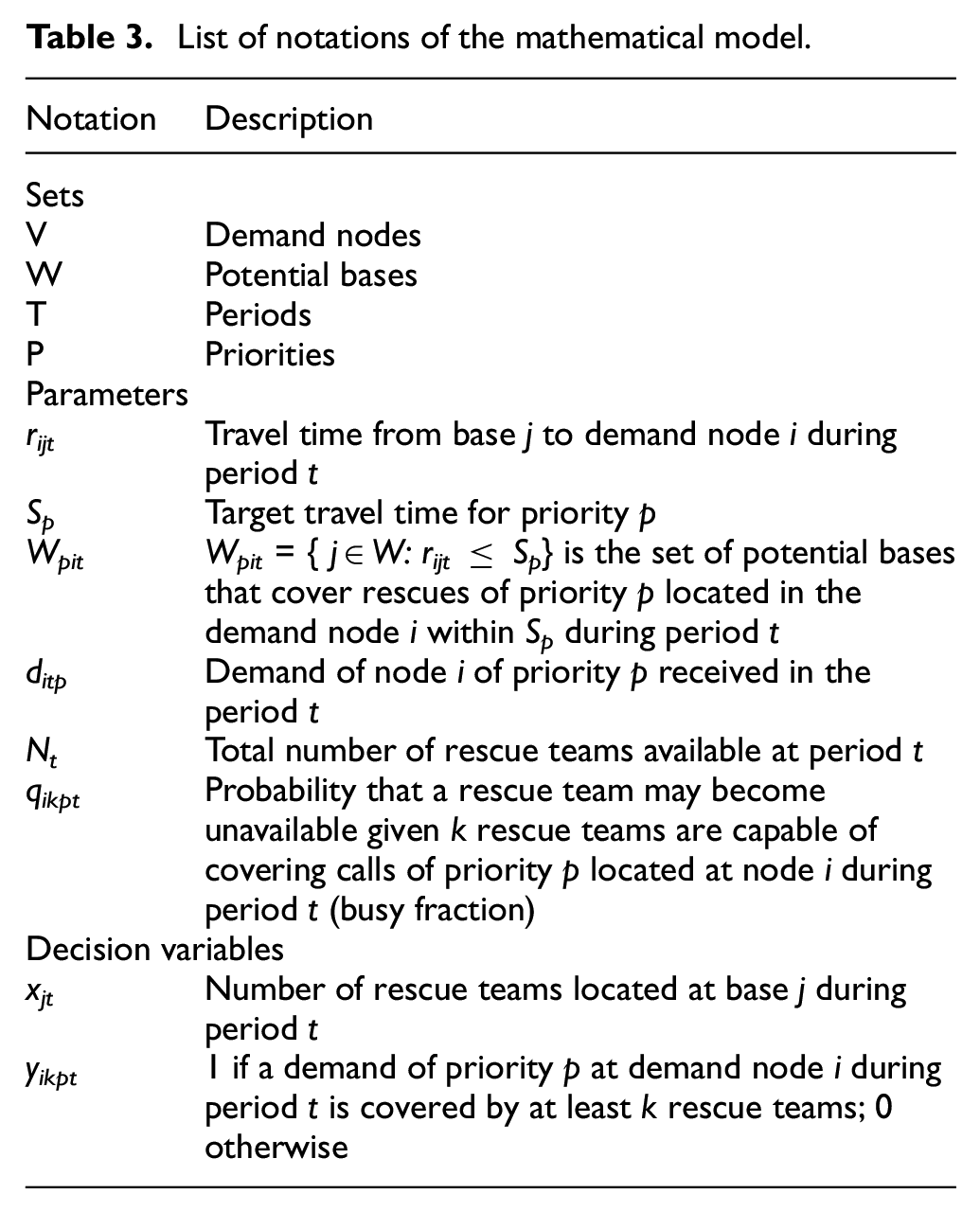
As mentioned above, the proposed iterative method encompasses a mathematical model and the DES model of the SAMU 94 to improve the overall coverage performance. The mathematical model is a multi-period extension of the MEXCLP of Daskin 18 that seeks to maximize the expected demand covered using a limited number of rescue teams. It integrates some specifics of the SAMU 94 system related to multiple rescue priority levels, multiple target travel time requirements and site-specific busy fraction estimates that depend on the number of rescue teams covering each demand node per period. Table 3 summarizes the notation used in the model.
List of notations of the mathematical model.
The model makes the following assumptions:
Demand points are aggregated, and bases are located using the IRIS structure, to be consistent with the DES model.
The colocation of rescue teams in the same home base is allowed. There are no capacity constraints for home bases.
The probability that a rescue team r1 is unavailable is independent of the probability that rescue team r2 is unavailable for all r1≠ r2.
The probability that a rescue team is busy is the same for all rescue teams eligible to serve the same demand node for the same priority at the same period.
The demand to be covered in the model corresponds to the total number of rescues received during the study period for each IRIS and each period.
Based on notation definitions, the mathematical multi-period SAMU 94 model can be formulated as follows:
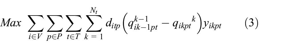


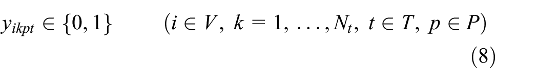
The objective function given by Equation (3) was built as follows: the probability of a rescue of priority p located in node i at period t is covered by a team given k rescue teams are capable of covering the node is
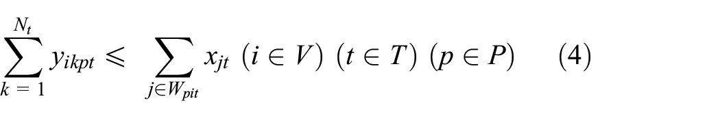
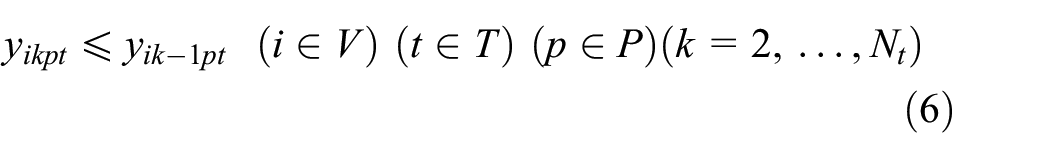
The first constraint given by Equation (4) defines the relationship between binary variables yikpt and integer variables xjt, by making sure that for each demand node, priority, and period, the total coverage provided by at least k rescue teams does not exceed the total number of rescue teams assigned to potential bases capable of covering this demand. The second constraint given by Equation (5) limits the total number of rescue teams that can be located to their scheduled capacity per period. The third constraint given by Equation (6) implies that a demand of priority p located at demand node i cannot be covered by at least k rescue teams if it is not covered by at least k–1 rescue teams during all periods. That is to say, if
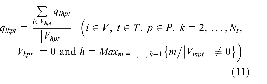
The probability that a rescue team may become busy, given k rescue teams are capable of covering calls of priority p located at node i during period t, can be estimated using the following equation:
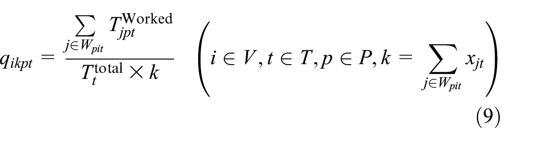
where
For a given simulation, if the number of rescue teams that cover a given demand point i for a certain priority p and period t is h, then the DES model will provide an estimate of
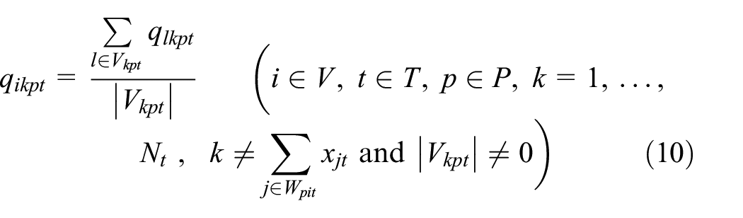
where
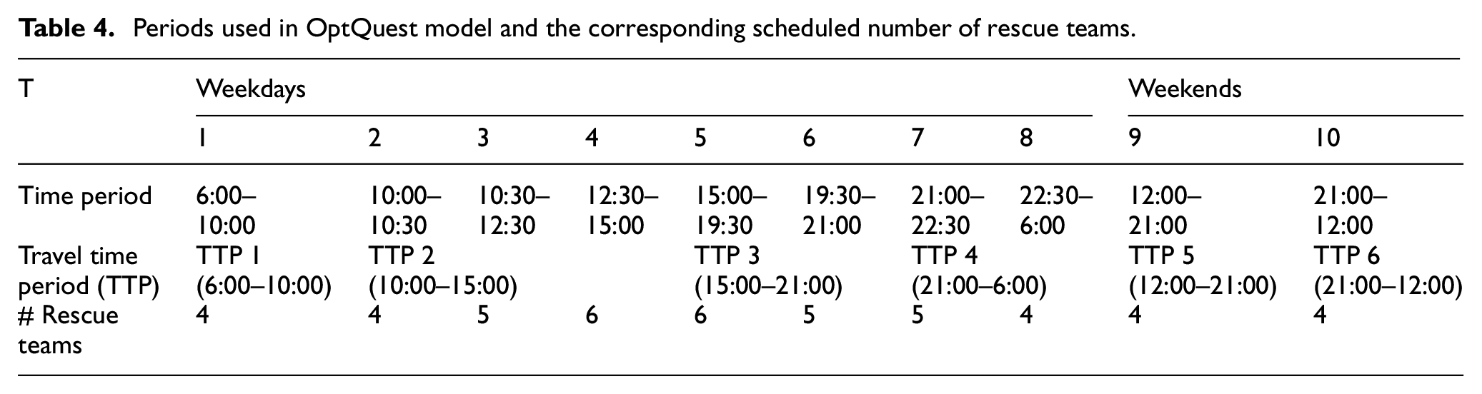
The Val de Marne department has 47 districts, whose centers were chosen as potential bases of the optimization problem. For the application of the mathematical model, we used 47 potential bases corresponding to the center of the 47 districts of the Val-de-Marne department and demand nodes corresponding to the 527 IRIS of the department. The six travel periods mentioned in section 3.2 were subdivided according to changes in the scheduled number of rescue teams, resulting in 10 time periods (Table 4). The coverage focuses on travel times because, as mentioned before, they are the response time component affected by redeployment decisions. Based on discussions with SAMU 94 managers, the thresholds of 5 and 10 min were set as working criteria for rescues of priority 1 and 2, respectively. For each target travel time, Wpit, which is the set of potential bases that cover rescues located in the demand node i during period t, was calculated.
Periods used in OptQuest model and the corresponding scheduled number of rescue teams.
4.2. The iterative method
The busy fractions
We used two termination criteria, and the optimization process ends if at least one of these criteria is satisfied:
Criterion 1: Location solution convergence, i.e., for two successive iterations n and n + 1,
Criterion 2: Maximum number of iterations (Nmax = 10).
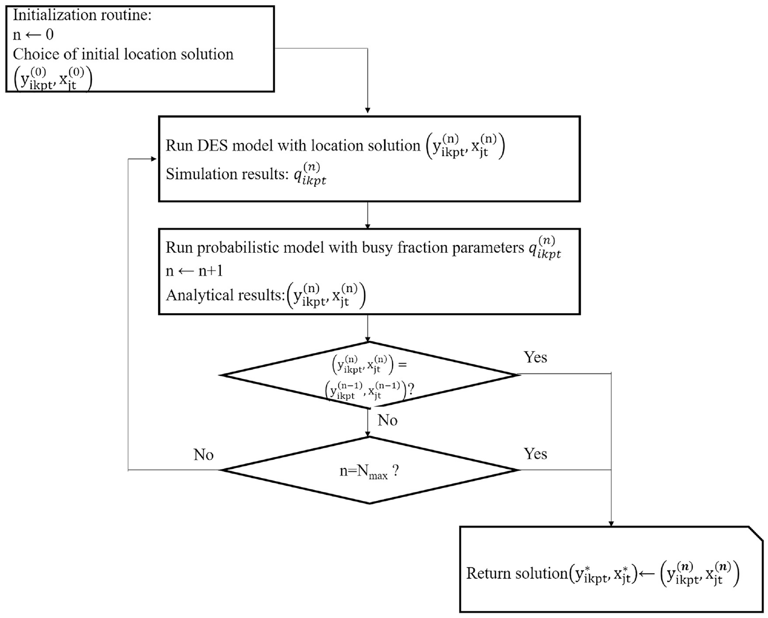
Iterative method procedure.
These criteria were used jointly to avoid the two major problems related to stopping conditions, described in the study by Nguyen et al., 10 which are: (1) the failure to converge to a stationary solution (too loose criteria) or (2) performing useless iterations, and therefore having an extra optimization time (too tight criteria).
In addition to termination criteria, there are several factors that affect the performance of the iterative method procedure such as the problem size (i.e., number of nodes, bases, periods, priorities), the length and number of replications of the DES model, but also the choice of the initial location solution
Figure 5 shows the graphical depiction of the percentage of calls covered within the target travel time estimated by the mathematical model (the orange curve) and the 95% confidence intervals of coverage within 20 min (the boxes show the 95% confidence interval for the metric, and whiskers show the best and worst cases of the 20 independent runs for each solution) obtained from the DES model through the iterations of the iterative method, for the 10 instances and the two priorities of rescues. The figure indicates that, among the 10 proposed instances, 7 converge according to criterion 1 (after 3 to 6 iterations), and 3 according to criterion 2 (after Nmax = 10 iterations). The same behavior has been observed for all instances and priorities: the more significant marginal improvements in simulated coverage performance had been achieved between the initial solution (iteration 0) and iteration 1 solution, achieving an average increase of 15.7% and 19,6% for priority 1 and 2, respectively. The subsequent iterations showed no or very few significant marginal differences between two successive iterations for both priorities and all instances. However, comparing the coverage performance of the last iteration with iteration 1 showed significant improvements for 4 instances over 10. These improvements achieved 1.9% on average, which demonstrated the interest in performing several iterations.
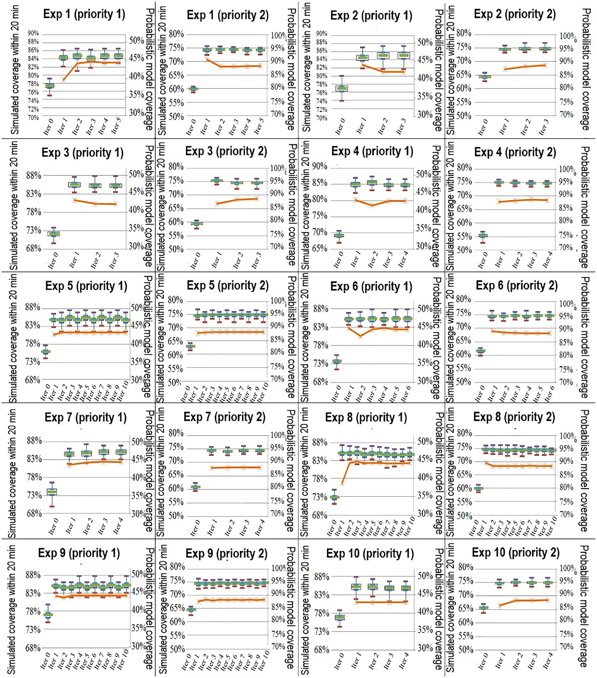
Iterative method results.
5. The OptQuest SAMU 94 model
To assess and compare the performance of the relocation solutions obtained by the iterative method described in section 4, we link the validated DES model described in section 3.2 with the optimization module OptQuest for Arena. An OptQuest model has three major elements: controls, responses, and objective. Controls are variables or resources of the DES model that can significantly affect system performance. Responses are outputs of the DES model that assess changes in controls. The objective is a mathematical expression involving the responses used to represent the optimization’s objective. OptQuest allows the use of constraints, which are linear/non-linear relationships among controls and/or responses, to increase the search’s efficiency. The SAMU 94 optimization problem in OptQuest can be summarized as follows.
5.1. Controls
Locations of rescue teams’ home bases per period.
5.2. Responses
R1 = number of priority 1 rescues reached within a target travel time of 5 min.
R2 = number of priority 2 rescues reached within a target travel time of 10 min.
R3 = total number of priority 1 rescues.
R4 = total number of priority 2 rescues.
5.3. Objectives
Maximize the percentage of calls reached within the target travel time, that is,
5.4. Constraints
No specified constraints.
5.5. Optimization options
Number of simulations: 500 simulations.
Tolerance value for determining when solutions are considered equal: 0.0001.
Number of replications per simulation: variable between 10 and 20.
For the application of the OptQuest model, we used the same data used in the iterative method: 47 potential bases corresponding to the center of the 47 districts of the Val-de-Marne department, demand nodes corresponding to the 527 IRIS of the department, 10 periods of time and a varying number of rescue teams (between 4 and 6) detailed in Table 4. The initial values of the controls correspond to the current location of rescue teams (i.e., VSG or HM). Similar to the iterative method, the objective function focuses on travel time target with the same thresholds (5 and 10 min for rescues of priority 1 and 2, respectively). The number of replications for each simulation was set to vary from 10 to 20. This option allows to rapidly weed out inferior solutions after 10 replications without wasting too much time on them. All simulations were carried out on Intel core i3—Processor 2.30 GHz and 4 GB RAM.
Figure 6 shows the progression of the best objective value using 500 simulations as a stopping criterion. The run time for one simulation of 10 to 20 replications is about 35 min. Therefore, an entire optimization run takes more than 12 days. The search procedure shows very little improvement in the objective value after 100 simulations, as depicted in the figure. Thus, the best value found at simulation 378 can be considered as a near-optimal solution.
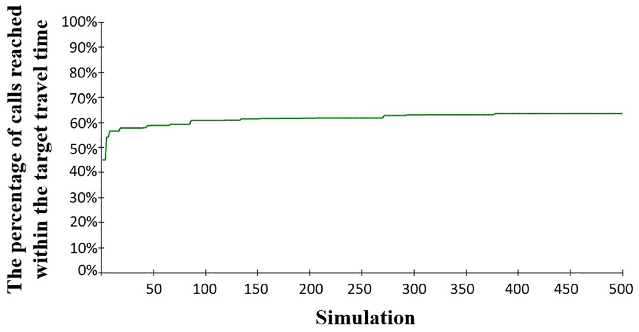
Optimization progression in OptQuest.
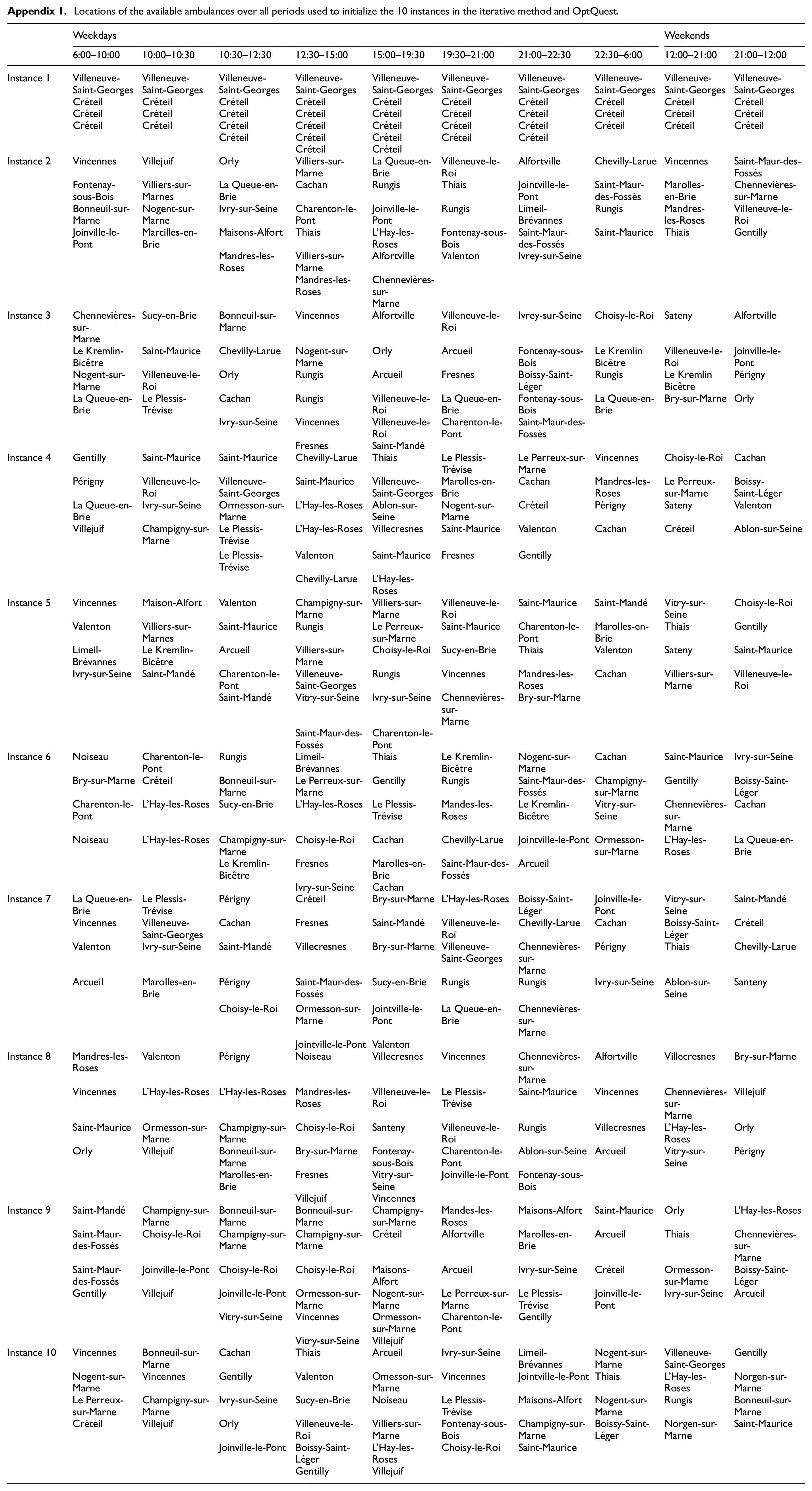
Several factors affect efficiency of the search for optimal solutions in OptQuest, such as the number of controls and their bounds, the number of replications and simulations, the complexity of the objective, and the initial values of the controls. 48 A good choice of the initial values can shorten the time it takes to find an optimal solution. Thus, similar to the iterative method, we used the current location of rescue teams (i.e., VSG or HM) and the same nine random location solutions used in section 4.2 to initialize controls (see Appendix 1). The solution of each instance was then evaluated using the DES model. To allow a fair comparison between instances, we do not change the stopping criterion (500 simulations) and the number of replications in OptQuest (10 to 20) at each run of the OptQuest algorithm. We also used the same DES model parameters (15 months of operations and 20 replicated times).
Figure 7 shows the results of the optimization solutions obtained from the 10 instances, along with the initial configuration of SAMU 94 (base case), regarding the metric “coverage within 20 min for rescues of priority 1 and 2.” This metric is a benchmark that has a particular interest for SAMU 94 managers. As seen in the figure, solutions of all 10 instances significantly improved the coverage performance. The improvements vary on average from 1.4% to 4.9% (respectively, 5.4% and 7.2%) for rescues of priority 1 (respectively, priority 2).
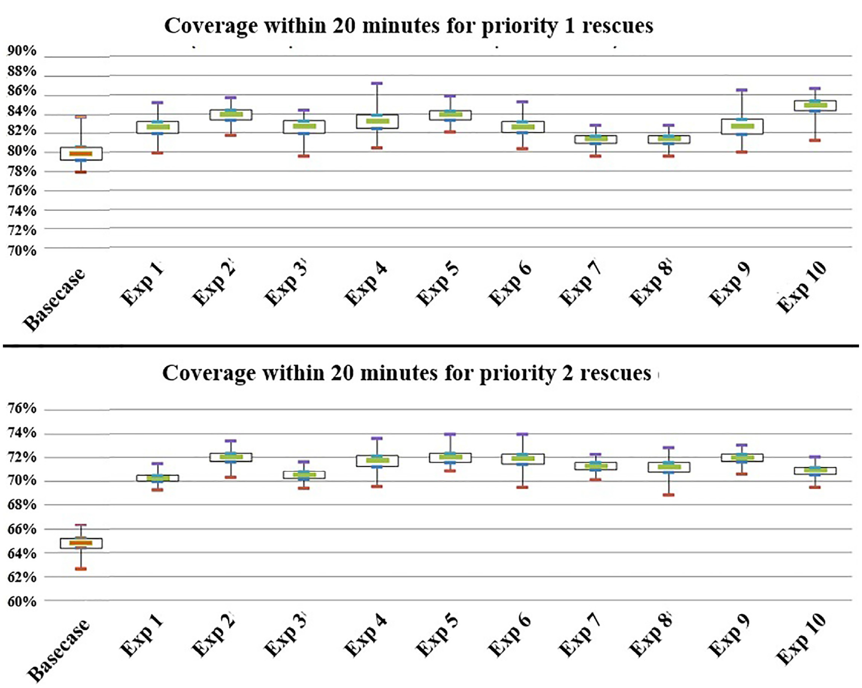
Coverage within 20 min for the base case and the optimization solutions obtained from the 10 instances.
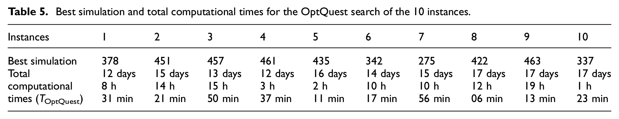
Furthermore, Table 5 illustrates the number of simulations needed to find the optimum solution by OptQuest and the total computational time for performing the search (TOptQuest). As observed in the table, when the initial solution changes, the number of simulations needed to find the optimum varies from 275 for instance 7, to 463 for instance 9. The total computational times also change from approximately 12 days for instance 4, to more than 17 days for instance 9. The average computational time for all instances is about 15 days, which is computationally very expensive, especially at the operational decision-making level. It is also worth mentioning that if the size of solution space increases (more potential bases, more rescue teams, more periods …), the computational time might dramatically grow in OptQuest. 42
Best simulation and total computational times for the OptQuest search of the 10 instances.
6. Experimental results
6.1. Computational times
The total computational time to perform the iterative method TIA corresponds to the time to run the DES model and the mathematical model for all iterations. The computational time needed to run the DES model changes from 104.5 to 248.4 min, with an average of 147.1 min, while the mathematical model is performed much faster with computational times varying from 3.4 to 8.2 min, with an average of 6.5 min. This results in an average TIA of 15 h 30 min, with great variability depending on the initial location (i.e., instance) and the corresponding number of iterations until convergence. The seven instances that converge according to criterion 1 have an average TIA of 10 h 17 min, while the three instances that converge according to criterion 2 have an average TIA of more than 26 h.
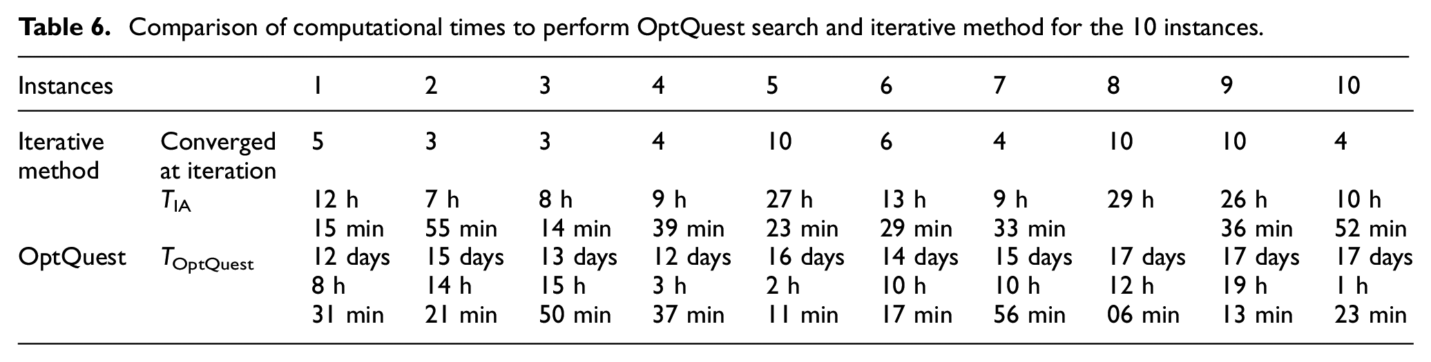
Table 6 illustrates the differences in computational times between the OptQuest search and the iterative method for each instance. The table shows that the computational times TIA have a large variability (i.e., a relative standard deviation of 55%) compared to TOptQuest (i.e., a relative standard deviation of 13.3%). Furthermore, we found that TIA was remarkably low since they represent 4.1% of the OptQuest computational time on average. This ratio is slightly larger for instances with convergence criterion 2, but it did not exceed 7.1% for all considered instances.
Comparison of computational times to perform OptQuest search and iterative method for the 10 instances.
6.2. Coverage performance
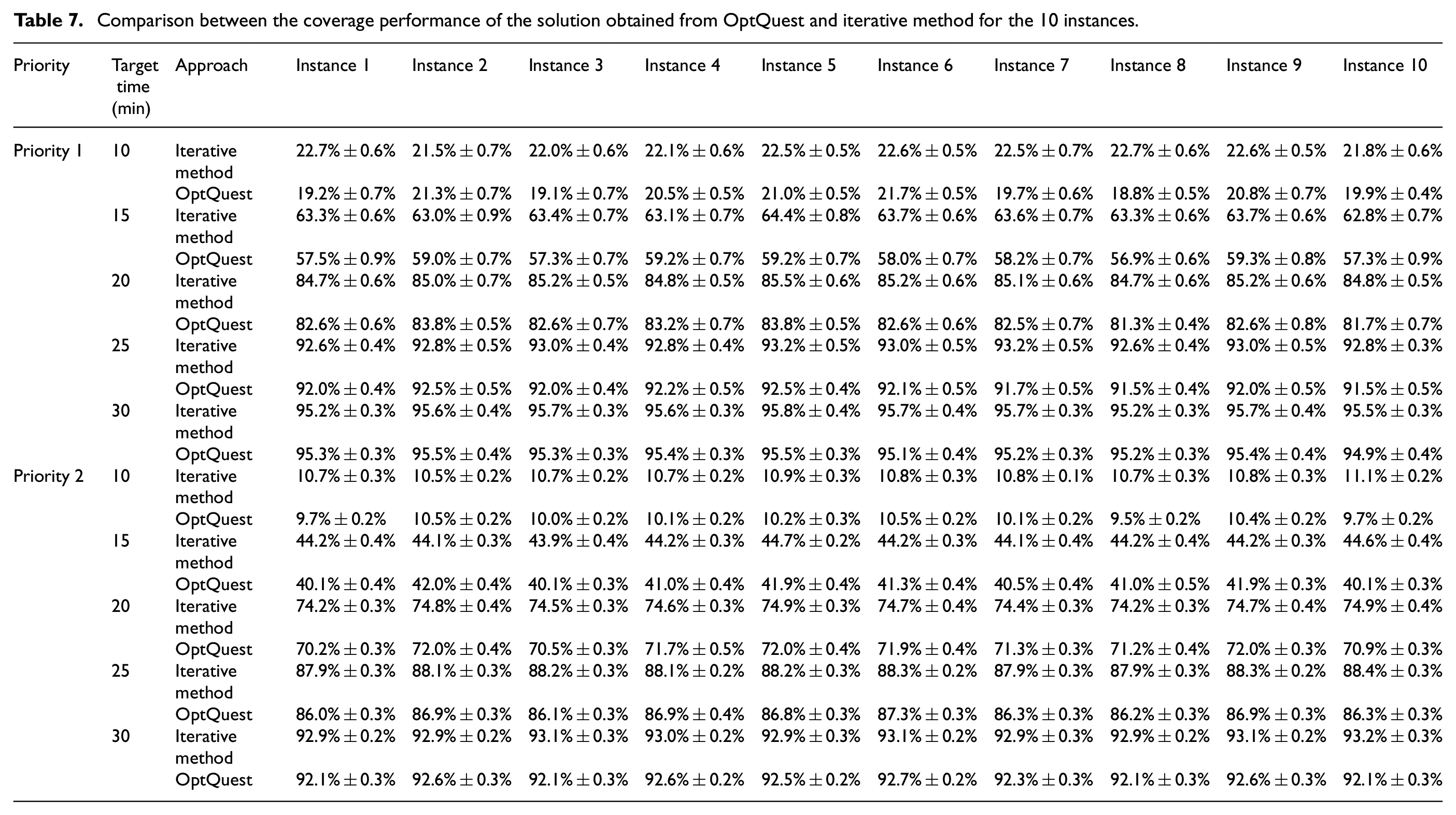
Table 7 shows confidence intervals of the simulated coverage of the location solutions obtained from the OptQuest search and the iterative method for the 10 instances. Several coverage target times (from 10 to 30 min) were analyzed to compare the solutions’ robustness over a wide range of response times. The comparison of the results shows that the iterative method generates better results than OptQuest for all instances. Specifically, the coverage within 15 and 20 min obtained from the iterative method solution was improved by 2.1% to 6.4% and 1.2% to 4%, respectively, compared to the OptQuest solution. For the target times 10 and 25 min, the iterative method outperforms OptQuest solution coverage by an average of 0.4% to 3.4% and 0.6% to 2.1%, respectively, for eight instances, while no significant differences in coverage were observed for the two remaining instances. There were very few significant differences in coverage within 30 min between OptQuest and the iterative method solution. They did not exceed 1.1% for all considered instances and priorities. This can be explained by the decrease of the effect of improving travel times (i.e., objective functions of the two approaches) as the coverage target time becomes larger.
Comparison between the coverage performance of the solution obtained from OptQuest and iterative method for the 10 instances.
As mentioned in the study by Nguyen et al., 10 a convergent DSBO process does not necessarily mean the global optimum has been found. The iterative method results confirm it since the coverage performances vary depending on the initial location solution. The solution of instance 5 outperforms the nine other instances for at least one coverage target time performance. Thus, even if it is not the optimal solution, instance 5 location solution would allow an interesting 15.7% and 14.4% average increase in coverage within 15 min for priority 1 and 2, respectively, and 5.6% and 10.1% average increase in coverage within 20 min for priority 1 and 2, respectively, compared to what is currently performed in the SAMU 94 system. Figure 8 displays the comparison of the coverage performance of the initial configuration of SAMU 94 (base case), with the instance 5 solutions obtained from OptQuest and the iterative method. As confirmed in this figure, the OptQuest solution performance remains lower than the iterative method solution performance. The difference in performance achieved 10.5% (respectively, 3.9%) and 11.7% (respectively, 7.2%) for the coverage target time of 15 min (respectively, 20 min) and priorities 1 and 2.
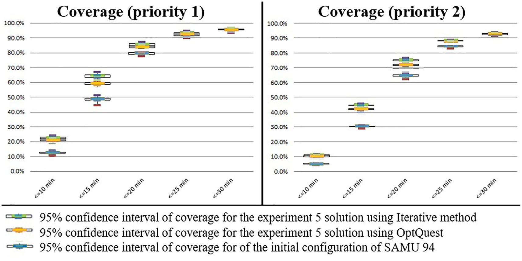
Comparison between the coverage performance of base case and instance 5 solutions obtained from OptQuest and the iterative method.
7. Summary and perspectives
This research demonstrated how DSBO could be applied to address the multi-period ambulance relocation problem, which can significantly increase coverage performance in EMSs. We proposed a DSBO approach applied to the Val de Marne department (France). This approach combines a multi-period mathematical model with a DES model integrated into an iterative method. The mathematical model seeks to determine the number and location of rescue teams for each period needed to ensure the maximum total expected coverage, while the DES model is used to compute busy fraction estimates needed to solve the mathematical model and to assess the system performance given the multi-period relocation solution obtained from the mathematical model.
The performance of the proposed iterative approach was compared to that of the DSBO software OptQuest for 10 instances corresponding to different initial solutions. The experimental results demonstrated that the iterative method is able to produce solutions with better coverage performance, 20 times faster than OptQuest on average. The improvements in coverage performance are particularly significant for lower coverage target times. For example, the best location solution obtained from instance 5 could increase the average coverage within 15 min up to 15.7% and 11.7% when using the iterative method and OptQuest, respectively, compared to the current SAMU-94 performance.
The practitioners facing similar multi-period redeployment problems in EMSs may prefer the use of easy-to-implement software packages such as OptQuest. It is probably a good idea when dealing with a very limited number of potential locations and periods, i.e., limited solution region. 49 When the solution region is large, our analysis shows that the proposed iterative method can be an efficient simulation-based optimization approach to address the multi-period redeployment problems and improve the EMS coverage performance in reasonable time, especially when enhancing the search performance with a good initial solution. A user interface will have to be developed to allow EMS practitioners to generate redeployment solutions without having the necessary operational research expertise to implement the proposed approach.
There are some limitations of the proposed methodology. First, the mathematical and DES models used historical demand data of the SAMU-94. Future research may consider using forecasts of emergency rescues’ number and geographical location to obtain sufficiently robust relocation solutions. It will also be worthwhile to look at the stopping criterion of the iterative method. Some instances show no significant improvement in coverage between the first and the last iterations, which indicates that useless iterations were performed. Future studies can, therefore, include a more comprehensive study on more efficient termination criteria that would allow fast convergence of the algorithm. In addition, the available computational infrastructure available to perform the study was weak, which strongly affected the computational times. Implementing the proposed iterative approach in better computational infrastructure would probably highly improve the runtimes, and therefore facilitate the application of the method to yield optimal solutions at the operational decision-making level. Finally, this study showed how mathematical modeling and DES could be used jointly to tackle complex multi-period redeployment problems. Future researches may consider other DSBO methods, 50 such as random search approaches or metamodels, to find the optimal/near-optimal relocation solution and to compare it with the results of the iterative method. Indeed, while such methods have been shown to be effective in the literature for small problem sizes (e.g., two input variables in the study by Maleyeff, 51 three input variables in the study by Cimellaro et al., 52 five input variables in the study by Zeinali et al. 42 ), more studies are needed to investigate their effectiveness in problems with larger solution space size such as the present relocation problem with 47 input variables.
Footnotes
Appendix
Locations of the available ambulances over all periods used to initialize the 10 instances in the iterative method and OptQuest.
| Weekdays | Weekends | |||||||||
|---|---|---|---|---|---|---|---|---|---|---|
| 6:00–10:00 | 10:00–10:30 | 10:30–12:30 | 12:30–15:00 | 15:00–19:30 | 19:30–21:00 | 21:00–22:30 | 22:30–6:00 | 12:00–21:00 | 21:00–12:00 | |
| Instance 1 | Villeneuve-Saint-Georges | Villeneuve-Saint-Georges | Villeneuve-Saint-Georges | Villeneuve-Saint-Georges | Villeneuve-Saint-Georges | Villeneuve-Saint-Georges | Villeneuve-Saint-Georges | Villeneuve-Saint-Georges | Villeneuve-Saint-Georges | Villeneuve-Saint-Georges |
| Créteil | Créteil | Créteil | Créteil | Créteil | Créteil | Créteil | Créteil | Créteil | Créteil | |
| Créteil | Créteil | Créteil | Créteil | Créteil | Créteil | Créteil | Créteil | Créteil | Créteil | |
| Créteil | Créteil | Créteil | Créteil | Créteil | Créteil | Créteil | Créteil | Créteil | Créteil | |
| Créteil | Créteil | Créteil | Créteil | Créteil | ||||||
| Créteil | Créteil | |||||||||
| Instance 2 | Vincennes | Villejuif | Orly | Villiers-sur-Marne | La Queue-en-Brie | Villeneuve-le-Roi | Alfortville | Chevilly-Larue | Vincennes | Saint-Maur-des-Fossés |
| Fontenay-sous-Bois | Villiers-sur-Marnes | La Queue-en-Brie | Cachan | Rungis | Thiais | Jointville-le-Pont | Saint-Maur-des-Fossés | Marolles-en-Brie | Chennevières-sur-Marne | |
| Bonneuil-sur-Marne | Nogent-sur-Marne | Ivry-sur-Seine | Charenton-le-Pont | Joinville-le-Pont | Rungis | Limeil-Brévannes | Rungis | Mandres-les-Roses | Villeneuve-le-Roi | |
| Joinville-le-Pont | Marcilles-en-Brie | Maisons-Alfort | Thiais | L’Hay-les-Roses | Fontenay-sous-Bois | Saint-Maur-des-Fossés | Saint-Maurice | Thiais | Gentilly | |
| Mandres-les-Roses | Villiers-sur-Marne | Alfortville | Valenton | Ivrey-sur-Seine | ||||||
| Mandres-les-Roses | Chennevières-sur-Marne | |||||||||
| Instance 3 | Chennevières-sur-Marne | Sucy-en-Brie | Bonneuil-sur-Marne | Vincennes | Alfortville | Villeneuve-le-Roi | Ivrey-sur-Seine | Choisy-le-Roi | Sateny | Alfortville |
| Le Kremlin-Bicêtre | Saint-Maurice | Chevilly-Larue | Nogent-sur-Marne | Orly | Arcueil | Fontenay-sous-Bois | Le Kremlin Bicêtre | Villeneuve-le-Roi | Joinville-le-Pont | |
| Nogent-sur-Marne | Villeneuve-le-Roi | Orly | Rungis | Arcueil | Fresnes | Boissy-Saint-Léger | Rungis | Le Kremlin Bicêtre | Périgny | |
| La Queue-en-Brie | Le Plessis-Trévise | Cachan | Rungis | Villeneuve-le-Roi | La Queue-en-Brie | Fontenay-sous-Bois | La Queue-en-Brie | Bry-sur-Marne | Orly | |
| Ivry-sur-Seine | Vincennes | Villeneuve-le-Roi | Charenton-le-Pont | Saint-Maur-des-Fossés | ||||||
| Fresnes | Saint-Mandé | |||||||||
| Instance 4 | Gentilly | Saint-Maurice | Saint-Maurice | Chevilly-Larue | Thiais | Le Plessis-Trévise | Le Perreux-sur-Marne | Vincennes | Choisy-le-Roi | Cachan |
| Périgny | Villeneuve-le-Roi | Villeneuve-Saint-Georges | Saint-Maurice | Villeneuve-Saint-Georges | Marolles-en-Brie | Cachan | Mandres-les-Roses | Le Perreux-sur-Marne | Boissy-Saint-Léger | |
| La Queue-en-Brie | Ivry-sur-Seine | Ormesson-sur-Marne | L’Hay-les-Roses | Ablon-sur-Seine | Nogent-sur-Marne | Créteil | Périgny | Sateny | Valenton | |
| Villejuif | Champigny-sur-Marne | Le Plessis-Trévise | L’Hay-les-Roses | Villecresnes | Saint-Maurice | Valenton | Cachan | Créteil | Ablon-sur-Seine | |
| Le Plessis-Trévise | Valenton | Saint-Maurice | Fresnes | Gentilly | ||||||
| Chevilly-Larue | L’Hay-les-Roses | |||||||||
| Instance 5 | Vincennes | Maison-Alfort | Valenton | Champigny-sur-Marne | Villiers-sur-Marne | Villeneuve-le-Roi | Saint-Maurice | Saint-Mandé | Vitry-sur-Seine | Choisy-le-Roi |
| Valenton | Villiers-sur-Marnes | Saint-Maurice | Rungis | Le Perreux-sur-Marne | Saint-Maurice | Charenton-le-Pont | Marolles-en-Brie | Thiais | Gentilly | |
| Limeil-Brévannes | Le Kremlin-Bicêtre | Arcueil | Villiers-sur-Marne | Choisy-le-Roi | Sucy-en-Brie | Thiais | Valenton | Sateny | Saint-Maurice | |
| Ivry-sur-Seine | Saint-Mandé | Charenton-le-Pont | Villeneuve-Saint-Georges | Rungis | Vincennes | Mandres-les-Roses | Cachan | Villiers-sur-Marne | Villeneuve-le-Roi | |
| Saint-Mandé | Vitry-sur-Seine | Ivry-sur-Seine | Chennevières-sur-Marne | Bry-sur-Marne | ||||||
| Saint-Maur-des-Fossés | Charenton-le-Pont | |||||||||
| Instance 6 | Noiseau | Charenton-le-Pont | Rungis | Limeil-Brévannes | Thiais | Le Kremlin-Bicêtre | Nogent-sur-Marne | Cachan | Saint-Maurice | Ivry-sur-Seine |
| Bry-sur-Marne | Créteil | Bonneuil-sur-Marne | Le Perreux-sur-Marne | Gentilly | Rungis | Saint-Maur-des-Fossés | Champigny-sur-Marne | Gentilly | Boissy-Saint-Léger | |
| Charenton-le-Pont | L’Hay-les-Roses | Sucy-en-Brie | L’Hay-les-Roses | Le Plessis-Trévise | Mandes-les-Roses | Le Kremlin-Bicêtre | Vitry-sur-Seine | Chennevières-sur-Marne | Cachan | |
| Noiseau | L’Hay-les-Roses | Champigny-sur-Marne | Choisy-le-Roi | Cachan | Chevilly-Larue | Jointville-le-Pont | Ormesson-sur-Marne | L’Hay-les-Roses | La Queue-en-Brie | |
| Le Kremlin-Bicêtre | Fresnes | Marolles-en-Brie | Saint-Maur-des-Fossés | Arcueil | ||||||
| Ivry-sur-Seine | Cachan | |||||||||
| Instance 7 | La Queue-en-Brie | Le Plessis-Trévise | Périgny | Créteil | Bry-sur-Marne | L’Hay-les-Roses | Boissy-Saint-Léger | Joinville-le-Pont | Vitry-sur-Seine | Saint-Mandé |
| Vincennes | Villeneuve-Saint-Georges | Cachan | Fresnes | Saint-Mandé | Villeneuve-le-Roi | Chevilly-Larue | Cachan | Boissy-Saint-Léger | Créteil | |
| Valenton | Ivry-sur-Seine | Saint-Mandé | Villecresnes | Bry-sur-Marne | Villeneuve-Saint-Georges | Chennevières-sur-Marne | Périgny | Thiais | Chevilly-Larue | |
| Arcueil | Marolles-en-Brie | Périgny | Saint-Maur-des-Fossés | Sucy-en-Brie | Rungis | Rungis | Ivry-sur-Seine | Ablon-sur-Seine | Santeny | |
| Choisy-le-Roi | Ormesson-sur-Marne | Jointville-le-Pont | La Queue-en-Brie | Chennevières-sur-Marne | ||||||
| Jointville-le-Pont | Valenton | |||||||||
| Instance 8 | Mandres-les-Roses | Valenton | Périgny | Noiseau | Villecresnes | Vincennes | Chennevières-sur-Marne | Alfortville | Villecresnes | Bry-sur-Marne |
| Vincennes | L’Hay-les-Roses | L’Hay-les-Roses | Mandres-les-Roses | Villeneuve-le-Roi | Le Plessis-Trévise | Saint-Maurice | Vincennes | Chennevières-sur-Marne | Villejuif | |
| Saint-Maurice | Ormesson-sur-Marne | Champigny-sur-Marne | Choisy-le-Roi | Santeny | Villeneuve-le-Roi | Rungis | Villecresnes | L’Hay-les-Roses | Orly | |
| Orly | Villejuif | Bonneuil-sur-Marne | Bry-sur-Marne | Fontenay-sous-Bois | Charenton-le-Pont | Ablon-sur-Seine | Arcueil | Vitry-sur-Seine | Périgny | |
| Marolles-en-Brie | Fresnes | Vitry-sur-Seine | Joinville-le-Pont | Fontenay-sous-Bois | ||||||
| Villejuif | Vincennes | |||||||||
| Instance 9 | Saint-Mandé | Champigny-sur-Marne | Bonneuil-sur-Marne | Bonneuil-sur-Marne | Champigny-sur-Marne | Mandes-les-Roses | Maisons-Alfort | Saint-Maurice | Orly | L’Hay-les-Roses |
| Saint-Maur-des-Fossés | Choisy-le-Roi | Champigny-sur-Marne | Champigny-sur-Marne | Créteil | Alfortville | Marolles-en-Brie | Arcueil | Thiais | Chennevières-sur-Marne | |
| Saint-Maur-des-Fossés | Joinville-le-Pont | Choisy-le-Roi | Choisy-le-Roi | Maisons-Alfort | Arcueil | Ivry-sur-Seine | Créteil | Ormesson-sur-Marne | Boissy-Saint-Léger | |
| Gentilly | Villejuif | Joinville-le-Pont | Ormesson-sur-Marne | Nogent-sur-Marne | Le Perreux-sur-Marne | Le Plessis-Trévise | Joinville-le-Pont | Ivry-sur-Seine | Arcueil | |
| Vitry-sur-Seine | Vincennes | Ormesson-sur-Marne | Charenton-le-Pont | Gentilly | ||||||
| Vitry-sur-Seine | Villejuif | |||||||||
| Instance 10 | Vincennes | Bonneuil-sur-Marne | Cachan | Thiais | Arcueil | Ivry-sur-Seine | Limeil-Brévannes | Nogent-sur-Marne | Villeneuve-Saint-Georges | Gentilly |
| Nogent-sur-Marne | Vincennes | Gentilly | Valenton | Omesson-sur-Marne | Vincennes | Jointville-le-Pont | Thiais | L’Hay-les-Roses | Norgen-sur-Marne | |
| Le Perreux-sur-Marne | Champigny-sur-Marne | Ivry-sur-Seine | Sucy-en-Brie | Noiseau | Le Plessis-Trévise | Maisons-Alfort | Nogent-sur-Marne | Rungis | Bonneuil-sur-Marne | |
| Créteil | Villejuif | Orly | Villeneuve-le-Roi | Villiers-sur-Marne | Fontenay-sous-Bois | Champigny-sur-Marne | Boissy-Saint-Léger | Norgen-sur-Marne | Saint-Maurice | |
| Joinville-le-Pont | Boissy-Saint-Léger | L’Hay-les-Roses | Choisy-le-Roi | Saint-Maurice | ||||||
| Gentilly | Villejuif | |||||||||
Funding
Financial support from the French National Research Agency (ANR) is gratefully acknowledged. Special thanks go to the SAMU-94 (EMS of the Val-de-Marne Department-France) for preparing the data, validating the DES model, and supporting this project.