A simulation model for resource allocation in port towage services

Abstract

In the face of developments in maritime transportation due to globalization, ports are tending toward new tugboat investments in order to respond to the increasing demand. Due to the high costs of tugboats, organizations may face high investment costs. It is important to determine the most suitable number of tugboats, considering the variables in a port area where towage services will be provided. In this study, a simulation model was developed to determine sufficient tugboat allocation according to some variables in ports. The simulation model was subjected to various experiments, and statistical analyses of the obtained results were performed. The relationships between the variables affecting the level of towage service were revealed.

Keywords

Tugboat allocation port services simulation modeling

1. Introduction

With the help of tugboats, maneuvering support is provided to ships and other marine vehicles that cannot safely maneuver by their own means in ports, on restricted waterways such as a strait or a canal, and on high seas. In port towage services, berthing and unberthing maneuvers of ships are assisted thanks to the push and pull capabilities of tugboats. While performing these services, tugboat masters follow the instructions of the marine pilot who is on board the ship. Pilotage and towage services, provided within the scope of technical–nautical services, are interdependent services.¹

It is important for ports to provide adequate towage services in terms of maritime safety and environmental protection. In a circular issued by the International Maritime Organization (IMO) in 2003, the importance of providing sufficient tugboat support in ports was emphasized in order to ensure sea and port safety, protect the marine environment, and relieve ship traffic. With this circular, IMO aimed to assist port authorities and port operators in assessing the adequacy of towage services.²

Ports and towage organizations are embarking on new tugboat investments in order to respond to the rapid developments in maritime transport. As an example of these developments, an increase in ship sizes and ship traffic, improvement of cargo handling equipment in ports, shortening of ships’ stay in ports, and so on can be given.³ According to UNCTAD (United Nations Conference on Trade and Development) statistics, the world merchant ship fleet has increased significantly in terms of “dead-weight tons” in recent years.⁴ For example, between 2019 and 2020, the world merchant ship fleet grew by 4.1%. Looking at the statistics of ships calling at ports, e.g., there was an increase of 6.07% between 2018 and 2019. Regarding the length of stay of ships in ports, e.g., there was a decrease of 0.41% between 2018 and 2019.⁵ In the face of these changes over the years, port towage service providers have renewed their tugboat fleets. Increased investments can result from more ship movements and faster fleet renewals, as well as innovations for energy-efficient tugboats. Since 2010, countries such as Turkey, the Netherlands, the United Kingdom, Italy, Germany, Spain, and Belgium have built a large number of new tugboats in about 10 years.⁶

It is important for towage service providers to pay attention to efficiency while making new investments, in terms of operating costs and service quality. The factors affecting the efficiency of towage services include number of tugboats (NT),^7,8 bollard pulls of tugboats,³ port area size,¹ waiting time of ships to receive towage services,^9,10 tugboats’ parking locations,¹ and frequency of ships arriving in port area.⁷ In addition, due to the high costs of tugboats, which are the sources of towage services, organizations are faced with high investment costs. Having more tugboats than necessary will cause an increase in investment and operating costs, and a decrease in efficiency as a result of the tugboats being idle. An insufficient NT will increase waiting times of ships and decrease service quality. For these reasons, it is necessary to determine the most suitable resource allocation, considering variables of a port area to be served. In this study, it is aimed to develop a simulation model for determining sufficient resource allocations in port towage services. In addition, it is aimed to reveal the relationships between the variables affecting the port towage service level.

In the next section, a literature review is given. In section 3, the method of the study is mentioned. The stages related to the development of the simulation model are explained in section 4. In section 5, the variables in the model and simulation experiments are mentioned. Statistical analyses of the simulation results and interpretation of the results are given in section 6. Section 7 is the discussion part of the study. In the conclusion, a general evaluation and suggestions for future studies are presented.

2. Literature review

Studies focused on towage services using simulation or optimization methods were examined. In general, it was seen that simulation studies consist of studies on port modeling and strait traffic modeling. It was determined that optimization studies mostly focus on tugboat scheduling and allocation problems in ports.

Optimization techniques such as particle swarm optimization,^11–13 evolutionary algorithm,^14–16 ant colony algorithm,^17–20 genetic algorithm,²⁰ and mixed integer programming^8,21,22 were used to solve tugboat scheduling and allocation problems. Yan et al.¹¹ proposed an improved particle swarm optimization algorithm for the tugboat scheduling problem. The proposed algorithm showed the advantages of faster convergence and better results than standard particle swarm optimization. Wang et al.¹² proposed a tugboat scheduling model and applied an improved discrete chaos particle swarm optimization algorithm to solve this problem. Wang et al.¹³ proposed an improved discrete particle swarm optimization algorithm for the tugboat assignment problem. The results showed that the proposed algorithm can provide better solutions than the genetic algorithm and the basic discrete particle swarm optimization algorithm. Liu¹⁴ used an evolutionary algorithm based on local search strategy for the optimization of the tugboat scheduling problem. The results showed that the algorithm is effective and applicable. Tao and Wenwen¹⁵ defined the tugboat scheduling problem as a kind of special parallel machine scheduling problem and made use of the evolutionary algorithm. Their algorithm provided an effective solution. Wenhui¹⁶ developed a heuristic simulation and optimization system for the allocation of tugboats in ports and used the evolution strategy to establish the optimization algorithm. Xu et al.¹⁷ formulated the tugboat scheduling problem as a multi-processor task scheduling problem. They proposed a simulated annealing–based ant colony algorithm to solve the problem. Wang and Meng¹⁸ applied ant colony optimization as an embedded optimization method to solve the tugboat scheduling problem. Wang et al.¹⁹ applied an improved trust-based ant colony optimization method to obtain the best tugboat scheduling plan. Their results showed that trust-based ant colony optimization can outperform basic ant colony optimization. Wang and Meng²⁰ developed a new heuristic method that combines genetic algorithm and ant colony optimization. They obtained satisfactory results regarding the performance of tugboat allocation optimization in container terminals. Wang et al.⁸ formulated a mixed integer programming model combined with a scheduling rule for the tugboat assignment problem in container terminals. Wei et al.²¹ developed a mixed integer linear programming model for the tugboat scheduling problem in container ports. Kang et al.²² proposed a tugboat scheduling problem, considering the uncertainty in ship arrival and towage service time, and developed a mixed integer linear programming model.

Apart from tugboat scheduling and allocation problems in ports or terminals, there are also optimization studies that deal with different problems. Bye and Schaathun²³ addressed the problem of dynamically positioning a tugboat fleet to reduce the risk of oil tanker drift accidents on the northern Norwegian coastline. They defined the tugboat fleet optimization problem as a one-dimensional model and presented a receding horizon genetic algorithm for its solution. In another study, Jaikumar and Solomon²⁴ examined the problem of minimizing the NT required to transport a certain number of barges between different ports in a river system. They considered the problem as a vehicle routing problem and used routing heuristics. To solve the problem, they developed a polynomial algorithm.

When the simulation studies were examined, it was seen that there are studies that focus entirely on towage services, as well as studies that examine towage services along with different subjects. In one of the simulation studies focusing entirely on towage services, Nas¹ aimed to determine the optimum parking locations of tugboats belonging to an organization providing towage services in a port in Turkey. Nas et al.⁷ developed a simulation model to examine the effect of maritime traffic in a port on the NT. Shahpanah et al.⁹ focused on the waiting time of ships for towage operations in container terminals and attacked the queuing problem in towage operations by simulation to reduce the average waiting time. Wang et al.²⁵ developed a simulation model to examine the optimal NT required under different handling capacity conditions of a port.

In some simulation studies, towage services are not the main research subject but are examined with different problems. Özbaş and Or²⁶ analyzed the effects of factors such as rules and regulations, NT and marine pilots, ship type, traffic density, and meteorological conditions on maritime traffic in the İstanbul Strait, by simulation. Uğurlu et al.¹⁰ examined Botaş Ceyhan Marine Terminal in terms of the number of arriving ships (NAS), queue values for berthing, ship waiting times for berthing, queue values for towage services, waiting time for towage services, total tugboat efficiency, etc. In a different research, Uğurlu et al.²⁷ performed a simulation study to evaluate the capacity of Tüpraşİzmit Tanker Terminal and to determine the amount of queues that may occur in terms of towage services. Ilati et al.²⁸ examined an integrated decision problem that deals with the simultaneous optimization of berth allocation, tugboat allocation, and quay crane assignment, and they used simulation and optimization methods together.

There is no study in the literature in which the appropriate tugboat allocation can be specified according to the variables of a port area and that presents a model that can be adapted to every port. This study aims to fill this gap in the literature.

2.1. Determining the variables and the performance measure

The variables and the performance measure to be examined in the study were determined by considering the relevant literature. In the study conducted by Nas et al.,⁷ it was emphasized that the determination of the NT that will provide the service level determined according to the dimensions of the authorization area is very important in terms of efficiency. The variables determined by considering their study are “NAS” and “NT.” When the study of Nas¹ was examined, it was seen that the size of the area where the organizations serve is an important factor in terms of service quality. The variable determined by considering Nas’s study is the “service area size (SAS).” Shahpanah et al.⁹ stated that ship waiting time is important in a port’s competitive advantage and focused on the waiting time of ships for towage services in container terminals. The performance measure and the variable determined from their study are “ship waiting time” and “NT,” respectively. Uğurlu et al.¹⁰ examined a terminal from many perspectives, one of which is the time that ships wait to receive towage services. The performance measure determined by considering their study is the “ship waiting time.” As a result, the variables that will be focused on in this study were determined as the NAS, the NT, and the SAS. The performance measure is the ship waiting time for towage services.

3. Methodology

Marine ports are complex systems, and it can be very difficult to analyze and solve problems in ports with analytical methods. Simulation is an essential tool used for modeling and analyzing processes, resources, and activities in ports. It helps decision-makers to achieve various goals such as increasing performance and efficiency in ports and reducing operating costs. Berth allocation and crane assignment in container terminals,²⁹ design and evaluation of container terminal configurations,³⁰ examination of the rail container processes,³¹ evaluation of cargo transfer alternatives in liquid cargo terminals,³² and so on can be given as examples of some port problems where simulation is used. These are just a few examples of port problems. It is known that simulation was used in many more port problems in the literature.

Towage operations in marine ports represent a discrete, dynamic, and stochastic system. System changes are dynamic since they evolve over time. A stochastic system exists since processes such as berthing and unberthing maneuvers with tugboats and ship arrivals are probabilistic. Since ships arrive and leave the system at certain times, the number of ships in the system changes at different points in time, in other words, discretely. The number of ships receiving towage services, the number of ships waiting for towage services, and the number of ships at the berth can be given as examples of discretely changing state variables. Considering these features of the port towage system, it was deemed suitable to use a discrete event simulation software. ProModel simulation software was used in this study.

The flow diagram showing the process of the study is given in Figure 1. Primarily, the problem of the research was determined. A literature review was conducted on studies using simulation or optimization methods in towage services. Considering the relevant literature, the variables to be examined in the study were determined. Then, a simulation model on port towage services was developed in ProModel simulation software. To determine the statistical distributions that will represent the random processes in the model, a literature review was made and the data of some ports in Turkey were examined. Then, the verification and validation of the model were checked. After the model development was completed, simulation experiments were designed. Experiment sets were developed from various combinations of the independent variables, and their simulations were run. Statistical analyses of the obtained simulation results were made. Afterward, some of the obtained simulation results were interpreted. As the final stage of the study, discussion and conclusion were mentioned.

Figure 1.

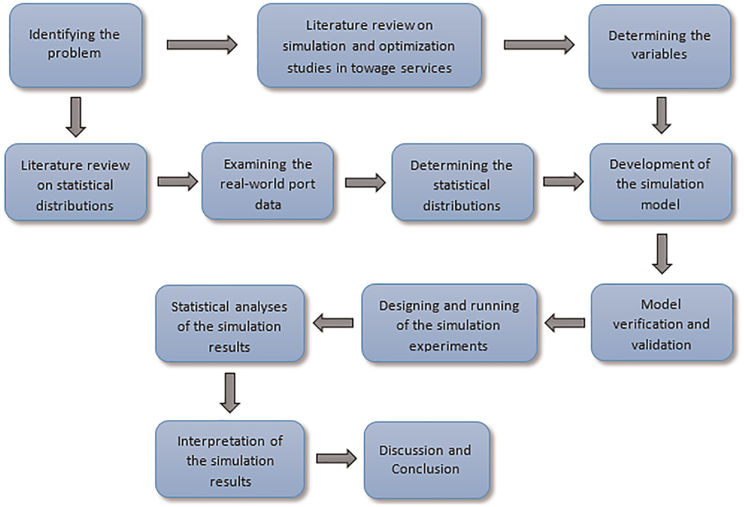
Flow diagram of the study.

4. Development of the simulation model

4.1. Conceptual model and assumptions

In the development phase of the simulation model, it would be appropriate to first give the conceptual model that provides a detailed description of the system to be examined. A conceptual model serves as a bridge between the definition of the problem and the simulation model.³³ Figure 2 shows a conceptual model of the system to be modeled in this study. It summarizes and visually presents the assumptions in the model.

Figure 2.

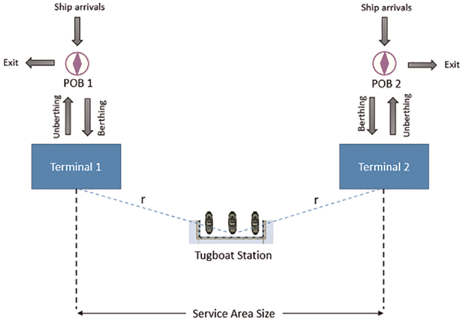
Conceptual model.

There are some assumptions about the simulation model to be developed. Considering Figure 2, these assumptions are as follows:

The port area in the model is a multi-purpose port area where more than one cargo type is handled.

There is no restriction on port capacity in the model. Ships arriving in the system can berth at any terminal in the port area to receive service.

There are two representative terminals in the port area. These terminals represent terminals located anywhere in a port area in real life. The average distance between all terminals was accepted as “r.”

The tugboat station was positioned in the middle of the towage service area. The distances from the tugboat station to the terminals are equal (r).

The distance between the two terminals furthest from each other in the port area was accepted as the “SAS.” The SAS was accepted as “2r,” with the tugboat station in the middle of the service area.

POB (Pilot on Board) positions are the locations where towage services begin (for berthing maneuvers) or end (for unberthing maneuvers).

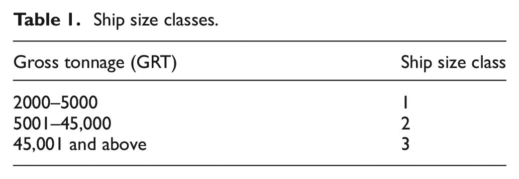
Ships that arrive at the system to receive service were divided into classes according to their sizes. While making the classification, the Regulation on Ports in Turkey was taken as a basis. According to the Regulation, all ships between 2000 and 5000 GRT (Gross Tonnage) must take at least one tugboat, all ships between 5001 and 45,000 GRT must take at least two tugboats, ships that do not carry dangerous goods over 45,000 GRT must take at least two tugboats, and ships that carry dangerous goods over 45,000 GRT must take at least three tugboats.³⁴ In this study, all ships over 45,000 GRT were considered as ships that take three tugboats. Consequently, in this study, ships were divided into three types of ship size classes based on their GRT (see Table 1).

There are no restrictions on the number and availability of marine pilots.

Tugboats in the model are of one type and port tugboats.

Table 1.

Ship size classes.

Gross tonnage (GRT)	Ship size class
2000–5000	1
5001–45,000	2
45,001 and above	3

4.2. Building the simulation model

Basic modeling elements in ProModel simulation software are entities, locations, resources, path networks, arrivals, and processing.³⁵ The basic modeling elements in the developed simulation model are as follows:

Entities: entities are the objects that enter the system, are processed or receive service, and leave the system. They may have characteristics such as speed, size, and condition. In this model, ships were defined as entities.

Locations: locations are places where entities are routed for processing, waiting, or decision-making. They possess a capacity for holding entities and may be available at certain times. Tugboat station, POB positions, terminals, ship arrival points, and exit points are locations of the present model.

Resources: resources are the elements used to process or transport entities. They may be static or dynamic. Tugboats were defined as dynamic resources in this model.

Path networks: it defines the paths in which resources and entities will follow. Necessary paths were defined between the locations in the present model.

Arrivals: information such as how often entities arrive in the system and at which location they enter the system are defined in the “Arrivals” section. In this model, ships enter the system at locations called ship arrival points.

Processing: it defines the routing of entities throughout the system and the operations that take place at each location they visit.

In the developed simulation model, advanced modeling elements of ProModel were also used in addition to the basic modeling elements. These advanced modeling elements are attributes, variables, and macros.

4.3. Algorithm of the simulation model

The algorithm showing the working principle of the simulation model is given in Figure 3. Ships enter the system according to the interarrival time distribution. Then, ships berth at one of the terminals with the required NT according to their size classes. If there are not enough tugboats available, ships wait at POB locations. Berthed ships stay at the terminal for loading and unloading operations according to the service time distribution. Ships which completed the operation process at the terminal perform unberthing maneuvers with the required NT according to their size classes. If there are not enough tugboats available, ships wait at the terminal until tugboats are available. Ships which performed unberthing maneuvers leave the system.

Figure 3.

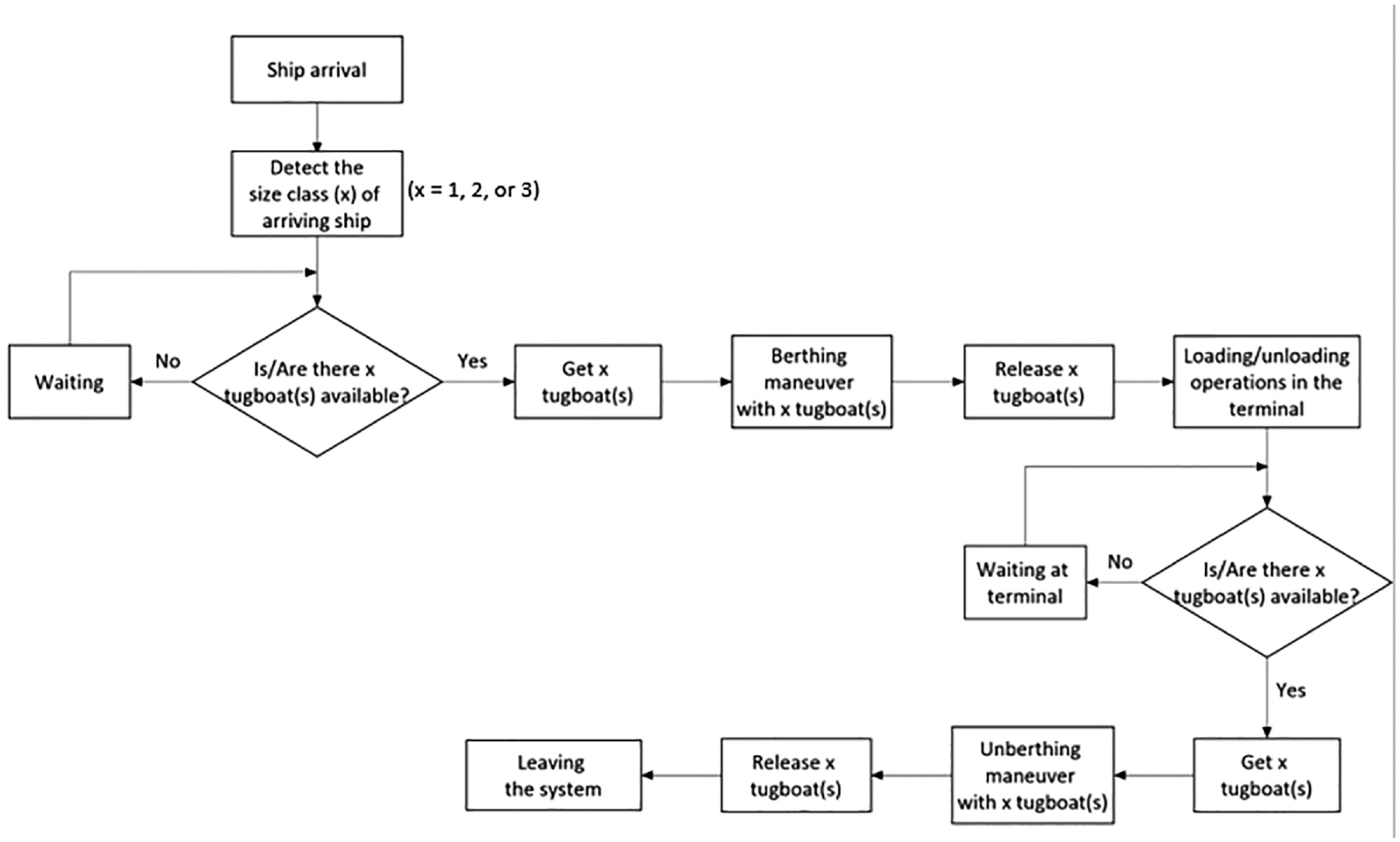
Algorithm of the simulation model.

Before the simulation is run, the tugboats are initially at the station. As time progresses, i.e., as ships arrive in the system, tugboats respond to the service requests of the ships and start to move. The time it takes for a tugboat to reach a ship is determined by the path distance and the tugboat’s own speed. Tugboats return to the station after serving the ships. They wait at the station when there is no service request.

When a ship requesting a tugboat needs to choose from the available tugboats, it selects the closest tugboat. On the contrary, when two or more ships request tugboats at the same time, tugboats choose the ship that has waited longest. Let us suppose that there is a ship waiting for a long time for two tugboats and there is another ship waiting for a shorter time for one tugboat. In such a case, when one tugboat becomes available, it chooses the ship that has waited longest.

4.4. Statistical distributions used in the model

The developed simulation model is a stochastic simulation model since it consists of various random processes. The random processes in the model are ship arrivals, berthing maneuver, service process at the berth, and unberthing maneuver. Statistical distributions related to these random processes are as follows:

Interarrival time distribution: it is the distribution of the differences between the times when ships arrive in the system.

Berthing maneuver time distribution: it is the distribution of the time spent by ships to berth to the terminal accompanied by tugboat(s).

Service time distribution: it states the distribution of the time spent by ships in the terminal to perform loading and unloading operations, and so on.

Unberthing maneuver time distribution: it denotes the distribution of the time spent by ships to leave from the terminal accompanied by tugboat(s).

Since the simulation model developed in this study is a theoretical model, there are no data about the system. For this reason, some statistical distributions were accepted for the above-mentioned random processes and were entered into the simulation model. To determine these distributions, a literature review was performed, and the distributions used in the studies were examined. Then, the data from different ports in Turkey were analyzed.

When the studies in the literature were examined, it was seen that the exponential distribution was mostly used for the interarrival time distribution.^36–39 It was also emphasized in some studies that the most adopted and used distribution for the interarrival time distribution of ships is the exponential distribution (Poisson process).^36,40,41 Therefore, in this study, the exponential distribution was preferred for the interarrival time distribution of ships.

For service time, the most common distribution in the simplest queuing systems is the exponential distribution. In some cases, service time distributions can be heavier tailed than the exponential distribution. To determine the service time distribution to be used in this study, three data sets related to ship operations belonging to three different port areas in Turkey were examined. The time elapsed between “ship berthed” and “ship departed” times in the data sets were calculated and the service time values of ships were obtained. The distributions representing these service time values were determined with the help of the Stat::Fit program included in the ProModel simulation software. The Stat::Fit program performs the Kolmogorov–Smirnov and Anderson–Darling goodness-of-fit tests. The best-fit distributions suggested by the Stat::Fit program for each data set were considered. As a result, it was seen that among the distributions that may be suitable for the service time of ships, there were tailed distributions such as “lognormal,”“loglogistic,” and “inverse Weibull.” In this study, it was deemed suitable to use the “lognormal” distribution as the service time distribution, since its parameters can be determined more easily than the others and it represents a tailed distribution.

A literature review was conducted on the distributions used for the berthing and unberthing maneuvers of ships. In most studies,^10,38,42,43 it was observed that deterministic values were used for these processes instead of statistical distributions. To determine the distributions that can be used for these processes, the above-mentioned data sets were examined. The goodness-of-fit tests was carried out in the Stat::Fit program. According to the test results, no suitable distribution was found for the berthing maneuver time and the unberthing maneuver time. As a result, empirical distributions were used instead of theoretical distributions to include the berthing maneuver and unberthing maneuver times of ships in the simulation model. The percentages of the time values were calculated in the data sets. Empirical distributions were defined by entering the time values and their percentages into the model.

Another distribution used in the simulation model is related to the speed of the tugboats. The normal distribution was used for the speed of tugboats traveling between any two locations. The speed of the tugboats was assumed to have a mean of 6 knots and a standard deviation of 1 knot in accordance with the normal distribution and was included in the simulation model with these parameters (1 knot = 1 nautical mile/hour).

4.5. Model verification and validation

Regarding the verification of the model, first, it was checked whether the commands in the operation logic and move logic sections in the “Processing” menu of the ProModel simulation software were written correctly. Then, the simulation was run and the processes in the model were monitored by slowing down the running speed. Ship arrivals, the NT taken by ships according to their size classes, movements with tugboats, and so on were checked. The values of the variables calculating the waiting times of ships off the terminal and at the terminal were checked by considering the simulation clock.

The validity of a simulation model is related to whether the model adequately represents the real-world system. Therefore, it is necessary to check whether simulation values of some determined performance measurements and real values are compatible. The simulation model developed in this study is not related to towage services belonging to an existing port in the real world. The model represents towage services in a general port area, and this study is a theoretical simulation study. However, in the model, ship arrivals, berthing maneuvers, service process at the terminal, and departure maneuvers occur similarly to their real-life counterparts. The results obtained from the simulation also support this situation. In addition, in section 7 of the study, some positive findings about the validity of the model are mentioned.

5. Design of experiments and running the simulation

5.1. Variables in the model

As mentioned before, the variables that will be focused on were determined by considering the relevant literature. Figure 4 shows the variables in the model. The independent variables in the model are as follows:

NAS: it is the variable related to the total number of ships arriving in the port area in a year.

NT: it is the total NT in the system that will serve ships during the berthing maneuver and unberthing maneuver processes.

SAS: it is the size of the port area served by tugboats in nautical miles. Tugboats travel between the station and various terminals to serve ships in a port area. The SAS mentioned in this study refers to the distance between the two furthest terminals in a port area. That is, the SAS indicates the boundaries of the port area served by tugboats.

The dependent variables in the model are related to the time that ships wait to receive towage services and these variables are as follows:

Waiting time off terminal (WOT): it denotes the variable related to the time in which ships arriving in the port area wait for the available tugboats at the POB locations, to berth the terminals. It refers to the response time of tugboats to the service request of ships located off the terminal.

Waiting time at terminal (WAT): it is the variable related to the time in which ships that have completed their operational processes wait for available tugboats, to leave the terminal. It states the response time of tugboats to the service request of the ships in the terminal.

Figure 4.

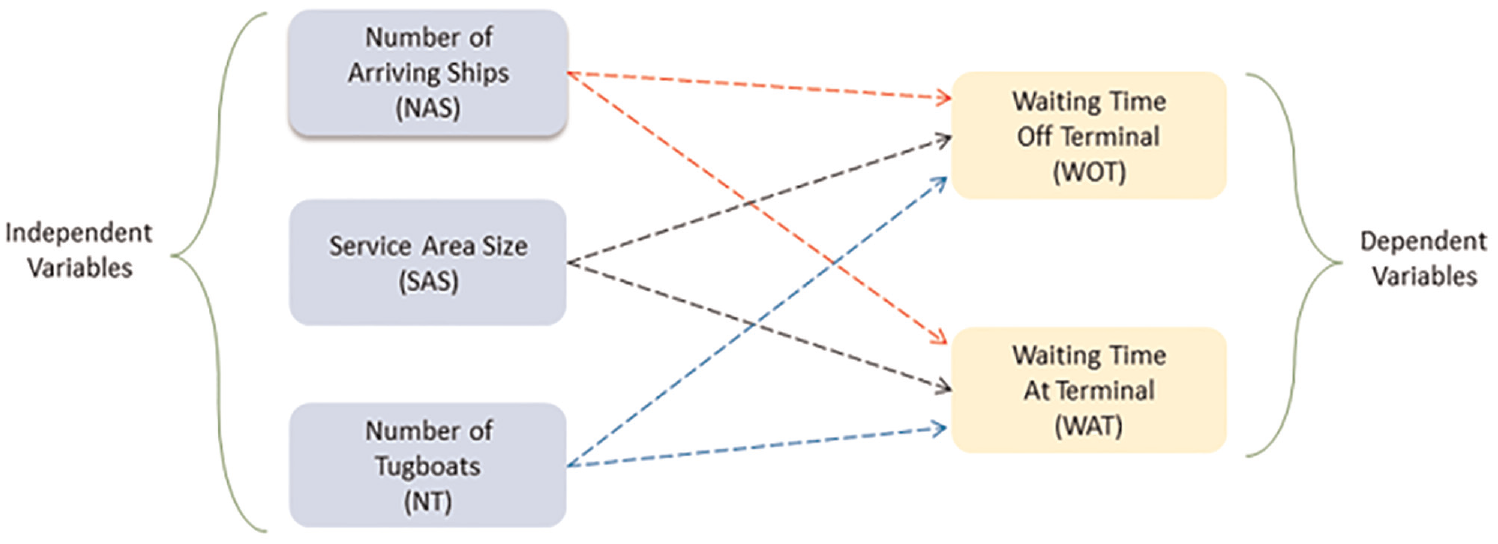
The variables in the model.

5.2. Running of simulation experiments

While designing the simulation experiments, the values of the independent variables NAS, SAS, and NT were changed at certain intervals. Table 2 shows the change intervals of the independent variables and the number of scenarios.

Table 2.

Simulation experiments.

Change intervals of the independent variables			Total number of scenarios
NAS	SAS (nautical mile)	NT
1000	1–10	3–5	30
2000	1–10	3–7	50
3000	1–10	3–7	50
4000	1–10	3–7	50
5000	1–10	3–7	50
6000	1–7	3–7	35
	8–10	4–8	15
7000	1–5	3–7	25
	6–10	4–8	25
8000	1–3	3–7	15
	4–9	4–8	30
	10	5–9	5
9000	1–2	3–7	10
	3–7	4–8	25
	8–10	5–9	15
10,000	1–6	4–8	30
	7–9	5–9	15
	10	6–10	5
Total = 480 scenarios

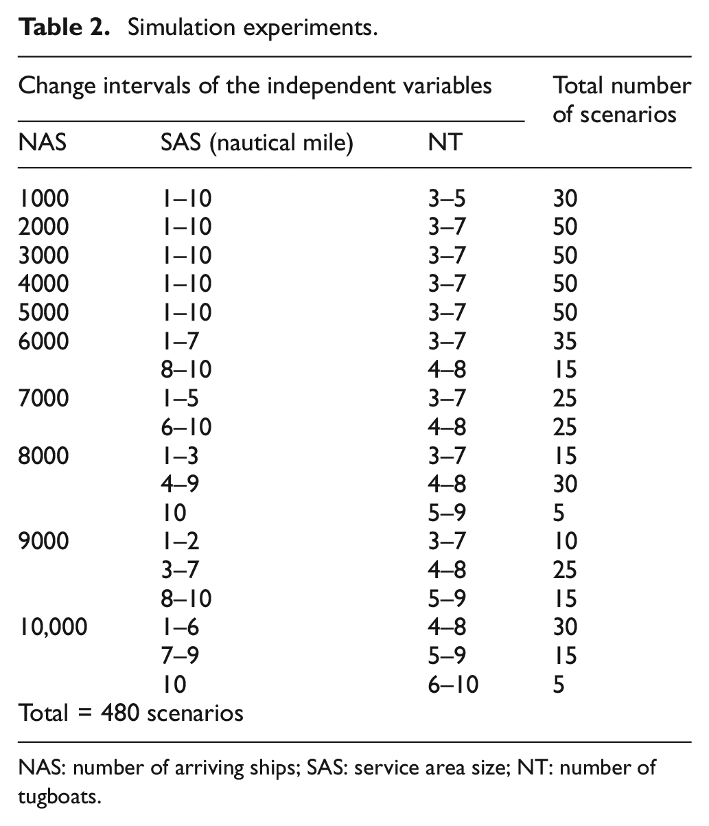
NAS: number of arriving ships; SAS: service area size; NT: number of tugboats.

In the scenarios, NAS was changed between 1000 and 10,000 in increments of 1000 ships. SAS ranges from 1 to 10 nautical miles for each NAS. NT varies in different intervals. For example, for a case where NAS is 7000 and SAS is 6 nautical miles, NT was considered starting with 4 tugboats, not 3. Because a simulation experiment with 7000 ships, 6 nautical miles, and 3 tugboats does not reach a steady state and does not give meaningful results. As a result, the scenarios, which do not reach a steady state and do not give meaningful results, were not considered. In addition, NT starts from a minimum of three tugboats in the scenarios. This is because there are ships in the model that request three tugboats at the same time.

While changing the NAS variable in the scenarios, the parameter of the exponential distribution, which is the interarrival time distribution, is also changed accordingly. Thus, the density of ships arriving in the port area within 1 year is changed. Consequently, changing the NAS variable means changing the density of ships.

For each scenario, the run time of the simulation was determined as 8760 h (1 year) and the warm-up time as 360 h (15 days). A total of 480 scenarios were simulated. The number of replications for each scenario was determined as 20. The simulation results of the WOT and WAT variables were obtained. These results are the averages of the results obtained from 20 replications of each scenario.

6. Statistical analyses and interpretation of simulation results

First, statistical analyses of the results obtained from the simulation experiments were carried out. Afterward, the simulation results were interpreted.

It is important for a good statistical analysis that the change intervals of the independent variables do not differ in the experimental sets consisting of combinations of independent variables. In addition, for the application of parametric analysis techniques, it is important to use normally distributed data or normally distributed data when a transformation is applied. For this reason, the experiments consisting of the change intervals of the independent variables shown in Table 3 were considered for the statistical analyses.

Table 3.

Experiments considered for statistical analyses.

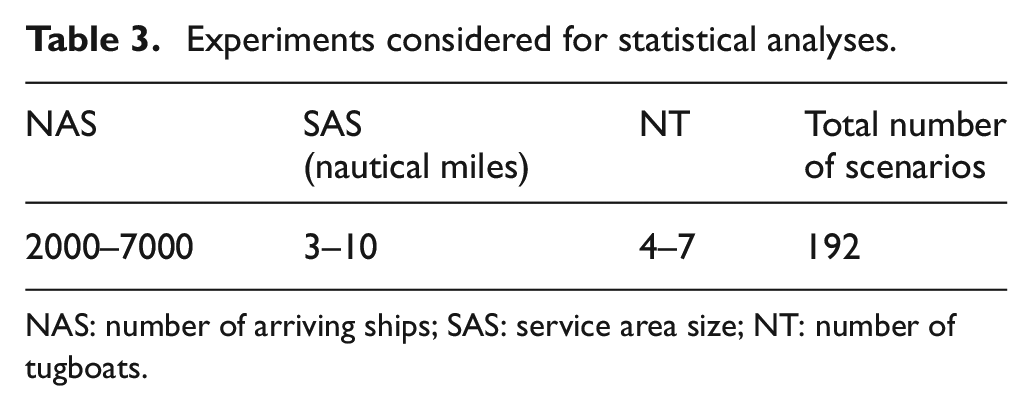
NAS	SAS (nautical miles)	NT	Total number of scenarios
2000–7000	3–10	4–7	192

NAS: number of arriving ships; SAS: service area size; NT: number of tugboats.

The results of a total of 192 scenarios, consisting of NAS varying between 2000 and 7000 ships (increments of 1000 ships), SAS varying between 3 and 10 nautical miles (increments of 1 nautical mile), and NT varying between 4 and 7 tugboats (increments of 1 tugboat), were subjected to statistical analyses. To perform these analyses, the SPSS program was used. On the contrary, the simulation results of all scenarios (480 scenarios) given in Table 2 were presented in Appendices 1 and 2 of the study.

6.1. Relationships between the variables

The Spearman correlation test was applied to examine the relationships between dependent and independent variables. Table 4 shows the results of the correlation test.

Table 4.

Correlation test.

Correlations
Spearman’s rho	Independent variables			Dependent variables
	NAS	SAS	NT	WOT	WAT
Independent variables
NAS
Correlation coefficient	1.000	0.000	0.000	0.619^a	0.205^a
Significance (two-tailed)		1.000	1.000	0.000	0.004
N	192	192	192	192	192
SAS
Correlation coefficient	0.000	1.000	0.000	0.449^a	0.931^a
Significance (two-tailed)	1.000		1.000	0.000	0.000
N	192	192	192	192	192
NT
Correlation coefficient	0.000	0.000	1.000	−0.616^a	−0.233^a
Significance (two-tailed)	1.000	1.000		0.000	0.001
N	192	192	192	192	192
Dependent variables
WOT
Correlation coefficient	0.619^a	0.449^a	−0.616^a	1.000	0.693^a
Significance (two-tailed)	0.000	0.000	0.000		0.000
N	192	192	192	192	192
WAT
Correlation coefficient	0.205^a	0.931^a	−0.233^a	0.693^a	1.000
Significance (two-tailed)	0.004	0.000	0.001	0.000
N	192	192	192	192	192

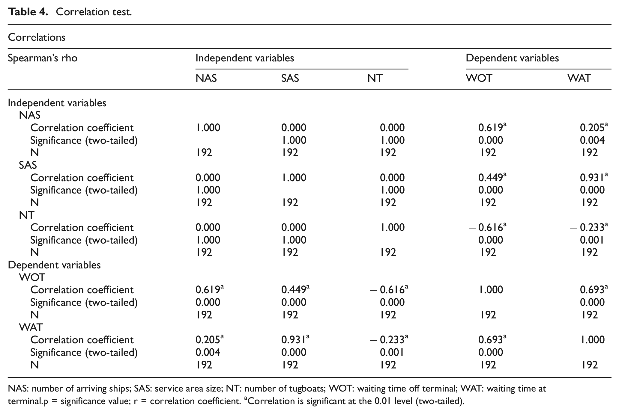
NAS: number of arriving ships; SAS: service area size; NT: number of tugboats; WOT: waiting time off terminal; WAT: waiting time at terminal. p = significance value; r = correlation coefficient. ^aCorrelation is significant at the 0.01 level (two-tailed).

A positive, moderate, and significant relationship was found between NAS and WOT (r = 0.619; p = 0.000). A positive, weak, and significant relationship was found between NAS and WAT (r = 0.205; p = 0.004). When the correlation coefficients were examined, it was seen that as NAS increased, WOT increased more than WAT.

A positive, moderate, and significant relationship was found between SAS and WOT (r = 0.449; p = 0.000). A positive, strong, and significant relationship was determined between SAS and WAT (r = 0.931; p = 0.000). It can be said that as SAS increases, WOT and WAT increase, but the increase in WAT is quite high.

A negative, moderate, and significant relationship was determined between NT and WOT (r = −0.616; p = 0.000). A negative, weak, and significant relationship was found between NT and WAT (r = −0.233; p = 0.001). It was determined that as NT increased, WOT decreased more than WAT.

6.2. Normality tests and data transformation

To apply parametric analysis techniques, the data should show a normal or close-to-normal distribution. Normality tests were performed to determine whether the simulation outputs show a normal distribution. SPSS program uses the Kolmogorov–Smirnov and Shapiro–Wilk for normality tests. Table 5 shows the results of the normality test of the WOT variable. The histogram graph of the WOT variable is shown in Figure 5.

Table 5.

Normality test results of the WOT.

Normality test
	Kolmogorov–Smirnov^a			Shapiro–Wilk
	Statistic	df	Significance	Statistic	df	Significance
WOT	0.282	192	0.000	0.541	192	0.000

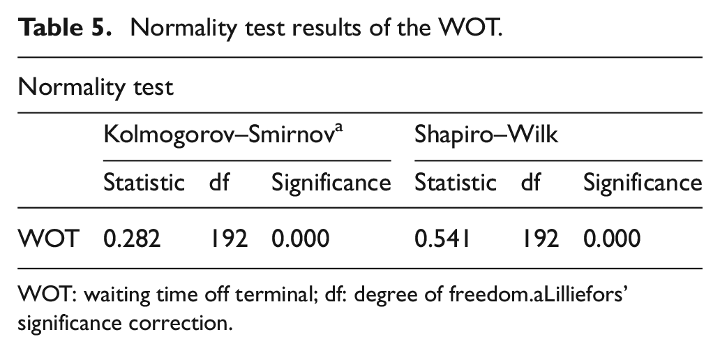
WOT: waiting time off terminal; df: degree of freedom. ^aLilliefors’ significance correction.

Figure 5.

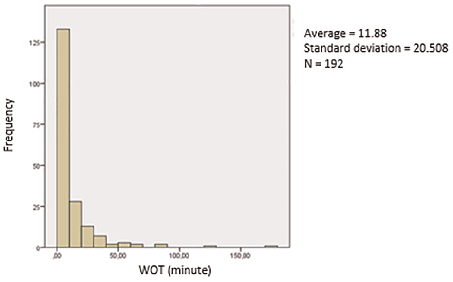
Histogram graph of WOT.

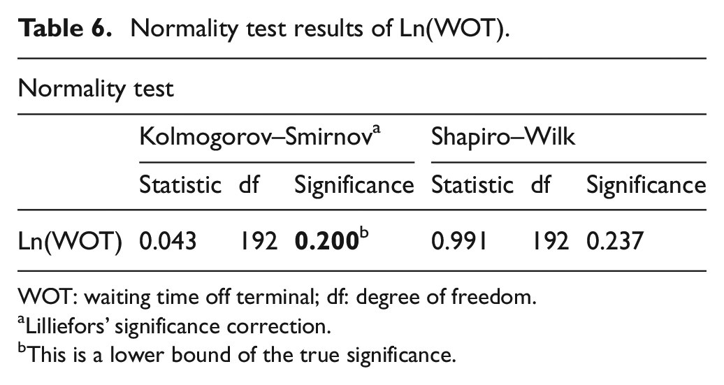
The significance values of Kolmogorov–Smirnov and Shapiro–Wilk tests for the WOT variable are 0.000. Accordingly, it was determined that the data of WOT were not normally distributed. Looking at the histogram graph in Figure 5, it is clearly seen that the data do not show a normal distribution. The logarithmic transformation was applied to the WOT variable. The normality test results of the Ln(WOT) variable are given in Table 6, and the histogram graph is given in Figure 6.

Table 6.

Normality test results of Ln(WOT).

Normality test
	Kolmogorov–Smirnov^a			Shapiro–Wilk
	Statistic	df	Significance	Statistic	df	Significance
Ln(WOT)	0.043	192	0.200 ^b	0.991	192	0.237

WOT: waiting time off terminal; df: degree of freedom.

Lilliefors’ significance correction.

This is a lower bound of the true significance.

Figure 6.

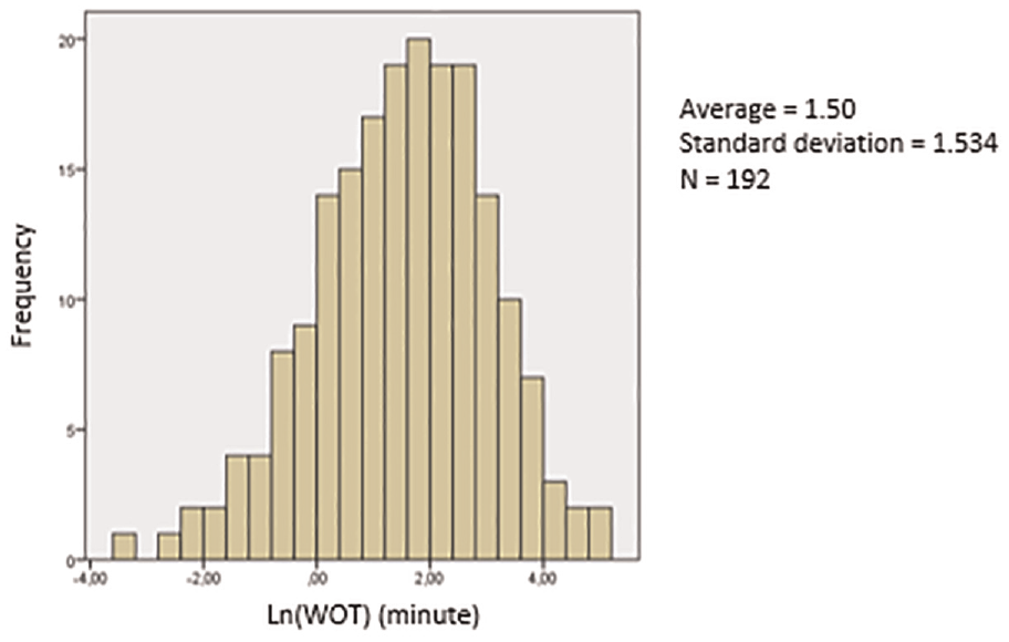
Histogram graph of Ln(WOT).

The significance values of Kolmogorov–Smirnov and Shapiro–Wilk tests for the Ln(WOT) variable are 0.200 and 0.237, respectively. Since these values are above 0.05, the data show a normal distribution with 95% confidence, according to both test results.

The normality test results of the WAT variable are given in Table 7, and the histogram graph is shown in Figure 7.

Table 7.

Normality test results of WAT.

Normality test
	Kolmogorov–Smirnov^a			Shapiro–Wilk
	Statistic	df	Significance	Statistic	df	Significance
WAT	0.124	192	0.000	0.798	192	0.000

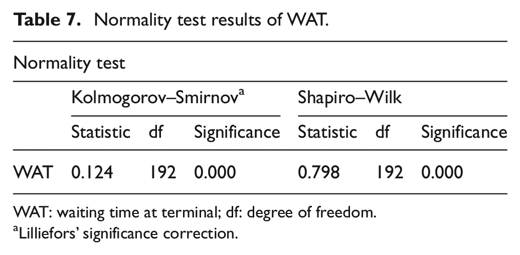
WAT: waiting time at terminal; df: degree of freedom.

Lilliefors’ significance correction.

Figure 7.

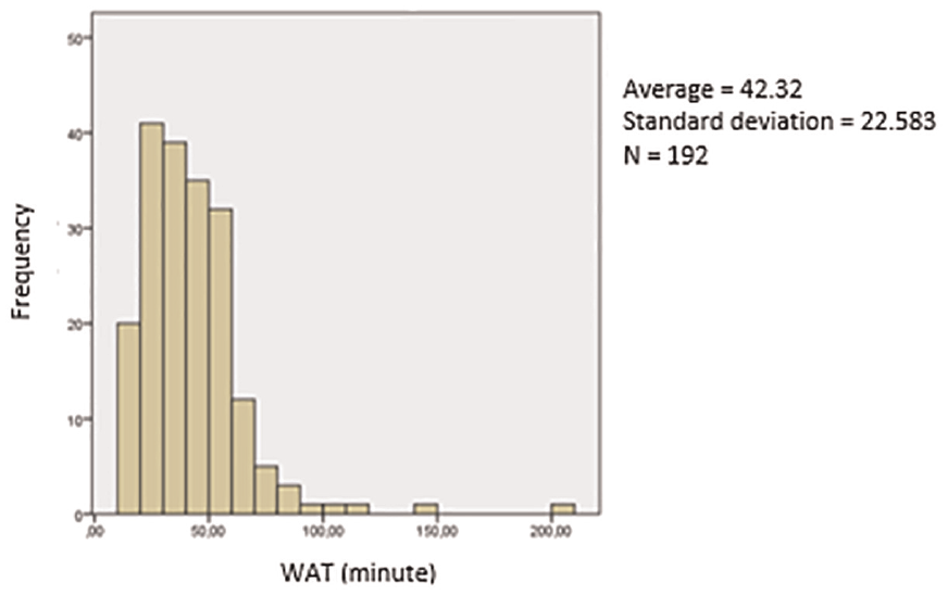
Histogram graph of WAT.

The significance values of Kolmogorov–Smirnov and Shapiro–Wilk tests for the WAT variable are 0.000. The data belonging to the WAT variable do not show a normal distribution. It can also be seen from the graph in Figure 7 that the data are not normally distributed. The logarithmic transformation was applied to the WAT variable. The normality test results of the Ln(WAT) variable are given in Table 8, and the histogram graph is given in Figure 8.

Table 8.

Normality test results of Ln(WAT).

Normality test
	Kolmogorov–Smirnov^a			Shapiro–Wilk
	Statistic	df	Significance	Statistic	df	Significance
Ln(WAT)	0.057	192	0.200^b	0.976	192	0.002

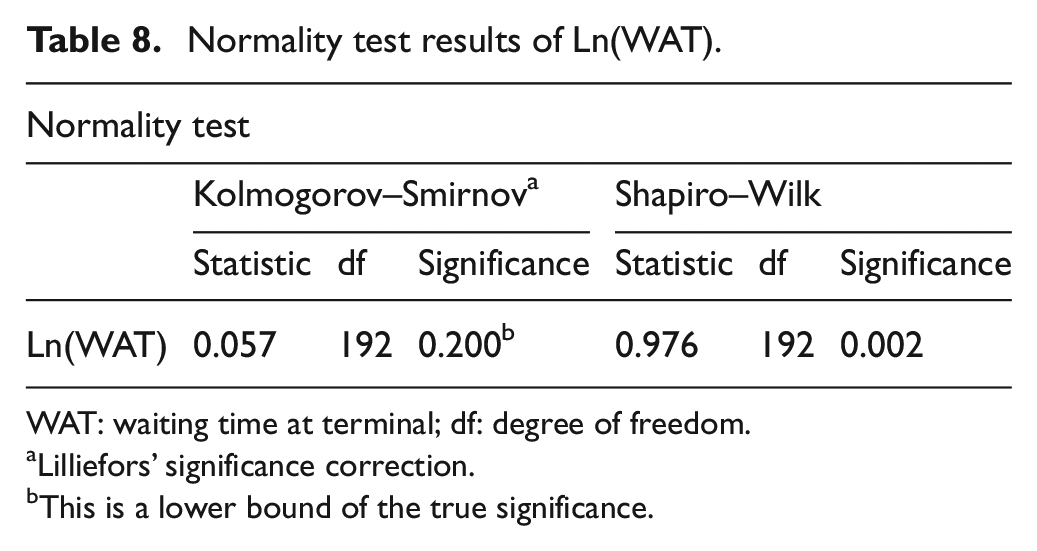
WAT: waiting time at terminal; df: degree of freedom.

Lilliefors’ significance correction.

This is a lower bound of the true significance.

Figure 8.

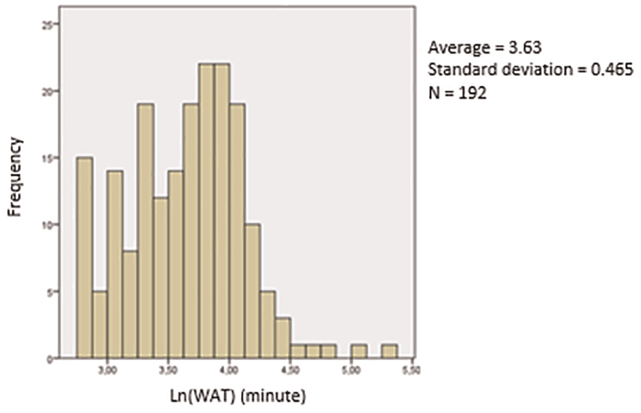
Histogram graph of Ln(WAT).

The significance values of Kolmogorov–Smirnov and Shapiro–Wilk tests for the Ln(WAT) variable are 0.200 and 0.002, respectively. According to the Kolmogorov–Smirnov test result, the data have a normal distribution with 95% confidence. By considering this test result, it was accepted that the data show a close to normal distribution. As a result, multiple linear regression analyses were performed using the dependent variables Ln(WOT) and Ln(WAT).

6.3. Multiple linear regression analyses

In this section, multiple linear regression analyses are presented which were performed to reveal the mathematical models of the relationships between the independent variables NAS, SAS, NT, and the dependent variables WOT and WAT.

To perform a multiple linear regression analysis, there should be no multi-collinearity problem which is the correlation between independent variables. Looking at the correlation test results in Table 4, it was seen that there is no relationship between NAS and SAS (r = 0.000; p = 1.000). No relationship was observed between NAS and NT either (r = 0.000; p = 1.000). Similarly, no relationship was found between SAS and NT (r = 0.000; p = 1.000). As a result, no multi-collinearity problem was found since there was no relationship between the independent variables.

6.3.1. Regression Model 1: the model where the dependent variable is WOT

A multiple linear regression analysis was performed between the independent variables NAS, SAS, NT, and the dependent variable Ln(WOT). Table 9 provides a summary of Regression Model 1.

Table 9.

Summary of Regression Model 1.

Model summary
Model	R	R square	Adjusted R square	Standard error of the estimate
1	0.989^a	0.979	0.978	0.22508

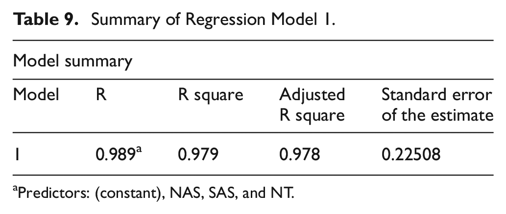
Predictors: (constant), NAS, SAS, and NT.

The R² value (0.979) shows that independent variables NAS, SAS, and NT considered together explain 97.9% of the change in the dependent variable Ln(WOT). Table 10 provides the results of the analysis of variance (ANOVA) test showing whether the regression model is significant.

Table 10.

The ANOVA test of Regression Model 1.

ANOVA^a
Model	Sum of squares	df	Mean square	F	Significance
1
Regression	440.017	3	146.672	2895.211	0.000^b
Residual	9.524	188	0.051
Total	449.541	191

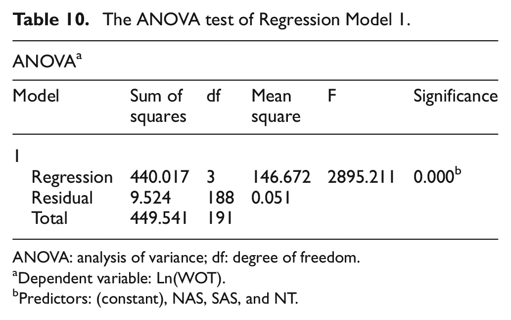
ANOVA: analysis of variance; df: degree of freedom.

Dependent variable: Ln(WOT).

Predictors: (constant), NAS, SAS, and NT.

Looking at Table 10, the significance level corresponding to the F value is 0.000. Since this value is less than 0.05, the model is significant, and it can be said that the regression model makes a statistically important contribution in explaining the dependent variable. Table 11 shows the results about the coefficients of the variables in the model.

Table 11.

Coefficients table of Regression Model 1.

Coefficients^a
Model	Unstandardized coefficients		Standardized coefficients	t	Significance
	B	Standard error	Beta
1
(Constant)	1.621	0.103		15.745	0.000
NAS	0.560	0.010	0.625	58.888	0.000
SAS	0.306	0.007	0.458	43.141	0.000
NT	−0.842	0.015	−0.615	−57.937	0.000

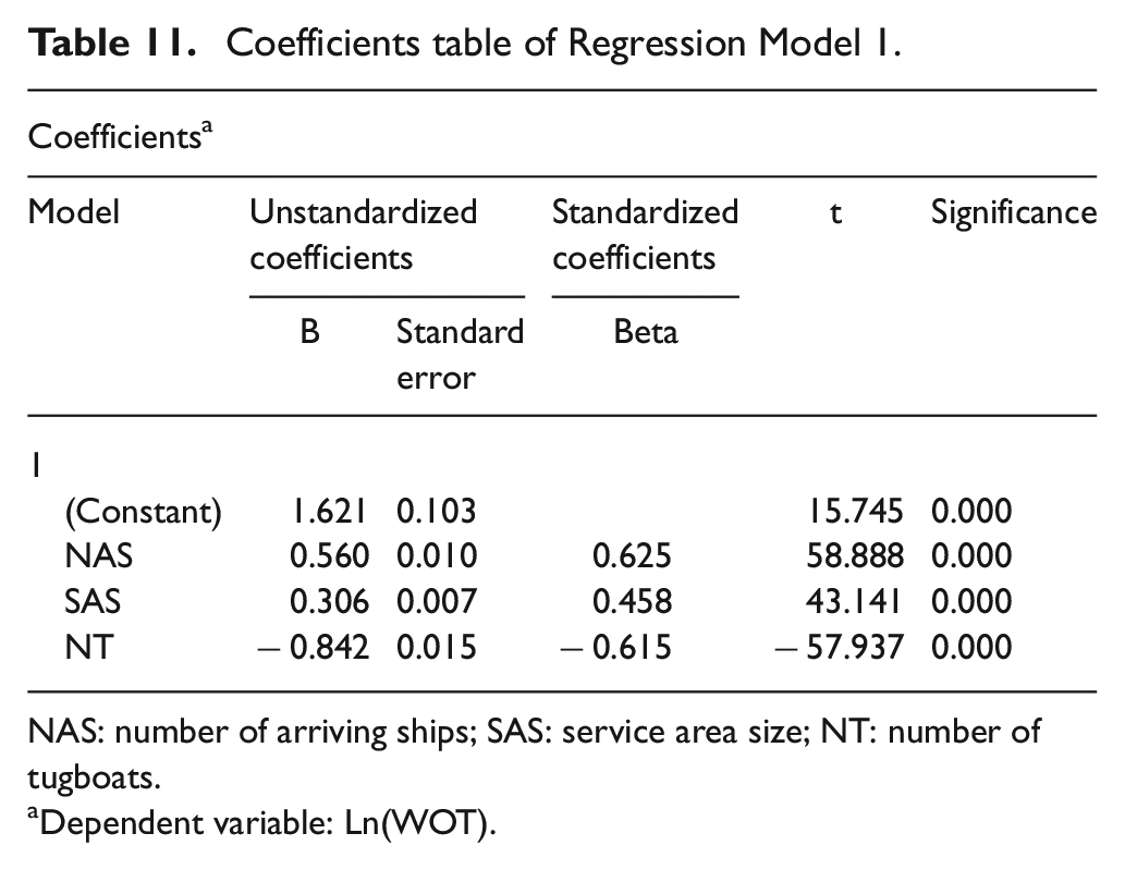
NAS: number of arriving ships; SAS: service area size; NT: number of tugboats.

Dependent variable: Ln(WOT).

It can be said that the NAS variable makes a statistically significant contribution to the explanatory value of the model (p = 0.000). The contribution of the SAS variable to the explanatory value of the model is also significant (p = 0.000). Similarly, the contribution of the NT variable to the explanatory value of the model is significant (p = 0.000). Since the measurement levels of the independent variables NAS, SAS, and NT are different, standardized beta coefficients were considered to make a healthy comparison between the variables in terms of explanatoriness. Among the independent variables, the most explanatory variables are NAS (beta = 0.625) and NT (beta = −0.615), followed by SAS (beta = 0.458). According to Table 11, the regression equation between the independent variables and the dependent variable WOT is expressed as follows:

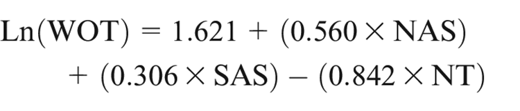
\begin{matrix} Ln (WOT) = 1.621 + (0.560 \times NAS) \\ + (0.306 \times SAS) - (0.842 \times NT) \end{matrix}

To examine the validity of the regression equation, the results obtained from the regression equation and the simulation results were compared. The values of the independent variables in 192 scenarios, which were taken into account in the statistical analyses, were used in the regression equation given above, and the results of the WOT variable were calculated. The scatter plot related to the simulation and regression results of the WOT variable is shown in Figure 9.

Figure 9.

The scatter plot related to the simulation and regression results of the WOT.

When Figure 9 is examined, it is seen that the values are distributed around a line close to 45°. Also, the value of R² = 0.988 is close to 1. Accordingly, it can be said that the regression equation related to the dependent variable WOT given above is valid.

6.3.2. Regression Model 2: the model where the dependent variable is WAT

A multiple linear regression analysis was performed between the independent variables NAS, SAS, NT, and the dependent variable Ln(WAT). The summary of the regression model is given in Table 12.

Table 12.

Summary of Regression Model 2.

Model summary
Model	R	R square	Adjusted R square	Standard error of the estimate
1	0.959^a	0.920	0.918	0.13290

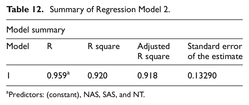
Predictors: (constant), NAS, SAS, and NT.

When Table 12 is examined, it is seen that the R² value is 0.920. This value shows that the independent variables NAS, SAS, and NT considered together explain 92% of the change in the dependent variable Ln(WAT). The ANOVA test is given in Table 13.

Table 13.

The ANOVA test of Regression Model 2.

ANOVA^a
Model	Sum of squares	df	Mean square	F	Significance
1
Regression	38.019	3	12.673	717.534	0.000^b
Residual	3.320	188	0.018
Total	41.340	191

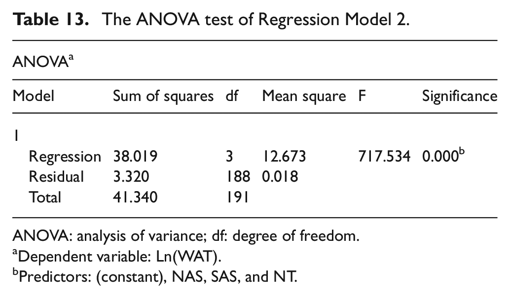
ANOVA: analysis of variance; df: degree of freedom.

Dependent variable: Ln(WAT).

Predictors: (constant), NAS, SAS, and NT.

The significance level corresponding to the F value is 0.000. The model is significant since this value is less than 0.05. This regression model presents a statistically important contribution in explaining the dependent variable. The results related to the coefficients of the variables in the model are shown in Table 14.

Table 14.

Coefficients table of Regression Model 2.

Coefficients^a
Model	Unstandardized coefficients		Standardized coefficients	t	Significance
	B	Standard error	Beta		Significance
1
(Constant)	2.759	0.061		45.378	0.000
NAS	0.061	0.006	0.223	10.795	0.000
SAS	0.182	0.004	0.897	43.419	0.000
NT	−0.105	0.009	−0.254	−12.282	0.000

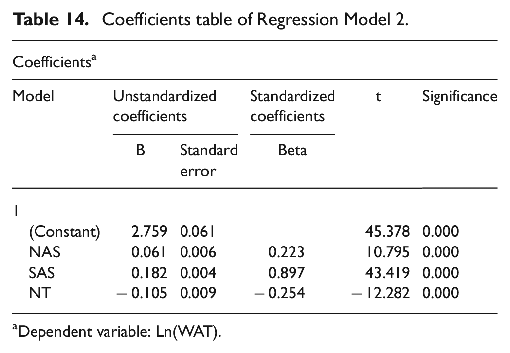
Dependent variable: Ln(WAT).

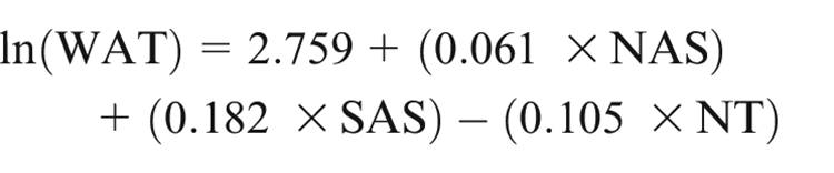
Each of the independent variables NAS, SAS, and NT make a statistically significant contribution to the explanatory value of the model (p = 0.000; p = 0.000; p = 0.000). According to the standardized beta coefficients, the most explanatory variable among the independent variables is SAS (beta = 0.897), followed by NT (beta = −0.254) and NAS (Beta = 0.223). According to Table 14, the regression equation between the independent variables and the dependent variable WAT is expressed as follows:

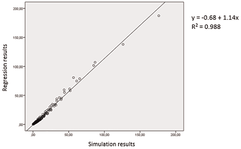
\begin{matrix} \ln (WAT) = 2.759 + (0.061 \times NAS) \\ + (0.182 \times SAS) - (0.105 \times NT) \end{matrix}

To check the validity of this regression equation, a comparison was made between the simulation results and the results of the regression equation. Figure 10 shows the scatter plot of the simulation and regression results of the WAT variable.

Figure 10.

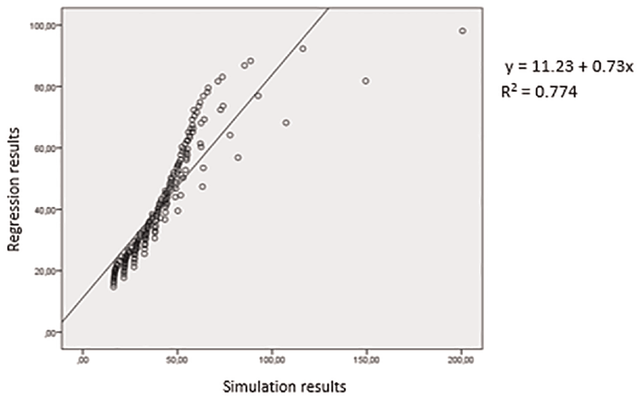
The scatter plot related to the simulation and regression results of the WAT.

It can be seen that the values are not distributed around a line of 45° or close to it. Therefore, the simulation and regression results of the WAT variable were examined. It was found that the regression equation does not adequately represent the simulation results for the values of WAT over 60 min. Simulation and regression results were compared for the values of WAT below 60 min. Figure 11 shows the scatter plot of this comparison.

Figure 11.

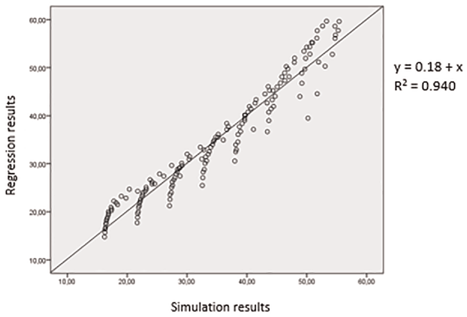
The scatter plot related to the simulation and regression results of the WAT values below 60 min.

If Figure 11 is examined, it can be seen that the values are distributed around a 45° line. Accordingly, it can be said that the regression equation related to the dependent variable WAT is valid for the values of the variable below 60 min.

6.4. Interpretation of simulation results

The WOT and the WAT variables were taken into account as performance measures for the interpretation of the simulation results. The results of all scenarios were not included in this section. As an example, the results where NAS is 5000 ships were interpreted. Simulation results of all scenarios were presented in Appendices 1 and 2.

For interpreting the simulation results, upper limits were determined related to WOT and WAT performance measures. To determine these upper limits, some marine pilots working in different ports in Turkey were consulted. By evaluating their opinions, some values were taken into consideration. The upper limit for the WOT variable was considered as 10 min. For the WAT variable, the upper limit was accepted to be 60 min. Consequently, these upper limits were determined for interpretation only and cannot be generalized at all.

First, the simulation results, where NAS is 5000 ships and the dependent variable is WOT, were examined. Figure 12 shows the graph of these results.

Figure 12.

Simulation results where the dependent variable is WOT and NAS is 5000 ships.

When the upper limit for the WOT variable was considered as 10 min, it is seen that at least four tugboats are required for service areas with 1, 2, and 3 nautical miles. For the service areas between 4 and 7 nautical miles, there should be at least five or six tugboats. In larger service areas, at least six or seven tugboats are required. Looking at Figure 12, it is seen that more than seven tugboats in large service areas do not significantly reduce the WOT.

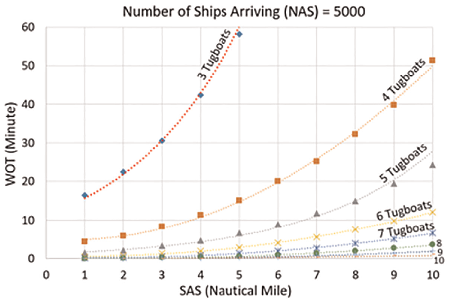
Second, the simulation results, where NAS is 5000 ships and the dependent variable is WAT, were examined. The graph of these simulation results is given in Figure 13.

Figure 13.

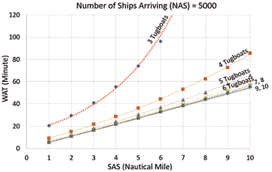
Simulation results where the dependent variable is WAT and NAS is 5000 ships.

When the upper limit for the WAT variable was considered to be 60 min, it is seen that three tugboats are sufficient in service areas up to 4 nautical miles. There should be at least four tugboats in service areas between 5 and 7 nautical miles and at least five tugboats in service areas with 8 and 9 nautical miles. At least six tugboats are needed for a service area with 10 nautical miles. It is seen that more than six tugboats in large service areas do not provide a significant reduction in the WAT variable.

7. Discussion

The results obtained from this study were compared with the data of a real port area. The port area compared is the port area in the Gulf of Gemlik in Turkey. According to the information received from the towage organization serving in this port area, there are six tugboats in service. According to the statistics of the General Directorate of Maritime Affairs for the year 2019, a total of 3490 ships visited the Port of Gemlik. The size of the port area is approximately 2.5 nautical miles (see Figure 14). On the contrary, according to the simulation results in this study, it is seen that at least three or four tugboats are sufficient when the NAS is 3000 or 4000 and the SAS is approximately 2.5 nautical miles (see Appendices 1 and 2).

Figure 14.

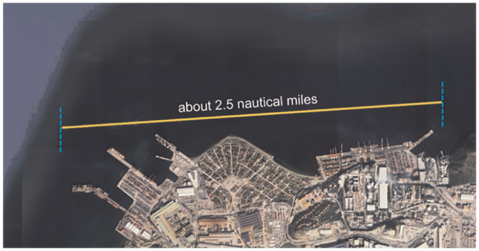
The Port of Gemlik and its size.

For the Port of Gemlik, the sufficient NT determined in this study and the NT currently in service were compared in terms of idle percentages. These idle percentages are given in Table 15.

Table 15.

Idle percentages of tugboats in recommended and current situations for the Port of Gemlik.

	Idle percentages
	Recommended number of tugboats		Existing number of tugboats
	Three tugboats	Four tugboats	Six tugboats
SAS = 2.5 nautical milesNAS = 3000 ships	65%	75%	83%
SAS = 2.5 nautical milesNAS = 4000 ships	55%	66%	78%

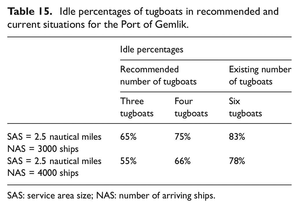
SAS: service area size; NAS: number of arriving ships.

In the case of 2.5 nautical miles and 3000 ships, the idle percentages are 65% and 75%, respectively, for 3 and 4 tugboats and 83% for 6 tugboats. In the case of 2.5 nautical miles and 4000 ships, the idle percentages are 55% and 66%, respectively, for 3 and 4 tugboats and 78% for 6 tugboats.

According to the simulation results in this study, when there are six tugboats in the Port of Gemlik, the tugboats are idle between 78% and 83%. In real life, according to 2019 data obtained from the towage organization in the Port of Gemlik, the average idle percentage of six tugboats is 87%. These data also show that tugboats are mostly idle. In addition, it is clear that the simulation results (78%–83%) are close to the real port data (87%). This situation showed that the developed simulation model approximately represents a real port and gave a positive result regarding the validation of the model.

In the study conducted by Nas et al.,⁷ the fact that the idle percentage of tugboats is approximately 50% indicates the sufficient NT according to the NAS. According to also Nas et al., it can be said that six tugboats are too many for the Port of Gemlik.

As a result, when making this comparison, bollard pulls of the tugboats, meteorological conditions, characteristics of the berths, and so on other factors were not considered. Considering all the factors that will affect towage services, ports should be modeled and examined according to their own characteristics.

8. Conclusion

The efficiency of the organizations that provide port towage services is important in terms of service quality, operating costs, navigational safety, and environmental protection. In this study, a simulation model was developed to determine the appropriate resource allocation for many situations consisting of different conditions in port towage services. Besides, the relationships between some variables affecting the service level were revealed. The results obtained from the developed model are expected to provide decision support for towage service providers.

In this study, it was tried to put forward a theoretical simulation model that can be adapted to every port. The model represents a general port area and was developed under certain assumptions. Ports need to be modeled and analyzed according to their own characteristics.

The purpose of the regression models in this study is only to show the relationships between the variables. If the waiting times of the ships are to be estimated, it would be better to consider the results of the simulation model rather than the regression models.

One of the limitations of this study is that it does not consider the bollard pulls of the tugboats. In future studies, it is recommended to take into account the bollard pulls of tugboats in experiments related to the NT. Besides, there is no restriction on the number of marine pilots in this study. Pilotage and towage services are interrelated services. For real port modelings, it will be useful to consider the number of marine pilots.

Footnotes

Appendix 1

Appendix 2 Acknowledgements

This study was derived from a doctoral thesis named “Optimization of Resources in Towage Services by Simulation Modeling Method.”⁴⁴ The thesis was prepared affiliated to Dokuz Eylül University, Graduate School of Social Sciences.

CORRECTION (September 2023): In Section 4.1 (Conceptual model and assumptions), column 2, the sixth bullet point was not needed, so this point has been deleted from the article.

Funding

This research received no specific grant from any funding agency in the public, commercial, or not-for-profit sectors.

ORCID iD

Emin Deniz Özkan

Author biographies

Emin Deniz Özkan is a full-time assistant professor in Dokuz Eylul University Maritime Faculty (Izmir, Turkey). He obtained his PhD in the Marine Transportation Engineering area. His studies focused on simulation modeling in maritime transportation, capacity analysis, and resource allocation in marine ports.

Selçuk Nas is a full-time professor in Dokuz Eylul University Maritime Faculty (Izmir, Turkey). His studies focused on “decision-making,”“risk management in maritime industry,”“ship operations,” and “safety of navigation,” and he gives consultancy support to the harbor pilotage organizations on risk assessment concerning ship maneuverings in harbor. He has been serving as a Board Member of the Turkish Chamber of Marine Engineers for 11 years.

References

Nas

Simulation optimization of the resources in technical/nautical services: selection of the parking locations of the tugboats. Dokuz Eylül Univ Marit Fac J 2013; 5: 57–81.

International Maritime Organization (IMO). Ship/port interface: availability of tug assistance (MSC/Circ.1101, MEPC/Circ.409, FAL/Circ.100), 2003, http://proamanaus.com.br/ohs/data/docs/3/Emprego_de_Rebocadores_em_Portos.pdf

Zorba

Nas

A study on determination of required tug force and number of tugs in port maneuvers. J ETA Marit Sci 2016; 4: 215–234.

United Nations Conference on Trade and Development (UNCTAD). Handbook of statistics (Sales No. E.21.II.D.1). New York: United Nations, 2020.

United Nations Conference on Trade and Development (UNCTAD). Review of maritime transport 2020 (Sales No. E.20.II.D.31). New York: United Nations, 2020.

European Tugowners Association (ETA). Economic impact of the European towage sector, https://eurotugowners.com/wp-content/uploads/2020/02/Final-report-Economic-impact-of-the-European-Towage-sector.pdf (accessed 10 April 2022).

Nas

Özkan

Uçan

The determination of the number of tugboats in the area of towage service authorization by using simulation modelling technique. J ETA Marit Sci 2016; 4: 91–99.

Wang

Kaku

Chen

, et al. Research on the modeling of tugboat assignment problem in container terminal. Adv Mater Res 2012; 433–440: 1957–1961.

Shahpanah

Hashemi

Nouredin

, et al. Reduction of ship waiting time at port container terminal through enhancement of the tug/pilot machine operation. J Teknol 2014; 68: 63–66.

10.

Uğurlu

Yüksekyıldız

Köse

Simulation model on determining of port capacity and queue size: a case study for BOTAS Ceyhan Marine Terminal. TransNav Int J Mar Navig Saf Sea Transp 2014; 8: 143–150.

11.

Yan

Bian

Chang

, et al. An improved particle swarm optimization algorithm for solving dynamic tugboat scheduling problem. In: Proceedings of 2009 2nd conference on power electronics and intelligent transportation system (PEITS 2009), Shenzhen, China, 19–20 December 2009, pp. 433–437. New York: IEEE.

12.

Wang

Zheng

, et al. An improved discrete particle swarm optimization for tugboat scheduling problem in container terminal. In: Proceedings of 3rd international conference on information management, innovation management and industrial engineering, Kunming, China, 26–28 November 2010, pp. 593–596. New York: IEEE.

13.

Wang

Zhu

Kaku

, et al. An improved discrete PSO for tugboat assignment problem under a hybrid scheduling rule in container terminal. Math Probl Eng 2014; 2014: 714832.

14.

Liu

Hybrid evolutionary strategy optimization for port tugboat operation scheduling. In: Proceedings of 2009 third international symposium on intelligent information technology application, Nanchang, China, 21–22 November 2009, pp. 511–515. New York: IEEE.

15.

Tao

Wenwen

Research of tugboat operation scheduling problem based on hybrid evolutionary strategy. In: Proceedings of the 2nd international conference on information science and engineering, Hangzhou, China, 4–6 December 2010, pp. 1438–1441. New York: IEEE.

16.

Wenhui

Heuristic algorithm for simulation and optimization system of port tugboats allocation. In: Proceedings of the 2011 international conference on internet computing and information services, Hong Kong, China, 17–18 September 2011, pp. 306–309. New York: IEEE.

17.

Mao

Jin

Simulated annealing-based ant colony algorithm for tugboat scheduling optimization. Math Probl Eng 2012; 2012: 246978.

18.

Wang

Meng

Simulation modeling and optimization for equipment scheduling in container terminals. In: Proceedings of the fifth IEEE international conference on cognitive informatics, Beijing, China, 17–19 July 2006, pp. 274–279. New York: IEEE.

19.

Wang

Zhu

Zheng

, et al. Tugboat scheduling problem based on trust-based ant colony optimization. In: Liu

Chang

(eds) Information computing and applications. Cham: Springer, 2012, pp. 373–380.

20.

Wang

Meng

Resource allocation and scheduling problem based on genetic algorithm and ant colony optimization. In: Zhou

Yang

(eds) Advances in knowledge discovery and data mining. Cham: Springer, 2007, pp. 879–886.

21.

Wei

Jia

Meng

, et al. Tugboat scheduling for container ports. Transp Res Part E 2020; 142: 102071.

22.

Kang

Meng

Tan

KC.

Tugboat scheduling under ship arrival and tugging process time uncertainty. Transp Res Part E 2020; 144: 102125.

23.

Bye

Schaathun

HG.

A simulation study of evaluation heuristics for tug fleet optimisation algorithms. In: chapter Werra

Parlier

Vitoriano

(eds) Operations research and enterprise systems. Cham: Springer, 2015, pp. 165–190.

24.

Jaikumar

Solomon

MM.

The tug fleet size problem for barge line operations: a polynomial algorithm. Transp Sci 1987; 21: 264–272.

25.

Wang

Zheng

Peng

The study of the influence of port scale on tugboat configuration based on system simulation. Adv Intell Syst Res 2018; 159: 4–7.

26.

Özbaş

Analysis and control of maritime transit traffic through the Istanbul channel: a simulation approach. Cent Eur J Oper Res 2007; 15: 235–252.

27.

Uğurlu

Yıldırım

Yüksekyıldız

, et al. An Awesim simulation study: to determine the efficiency of future improvements on Tupras Izmit Oil terminal. J Shipp Ocean Eng 2015; 5: 271–279.

28.

Ilati

Sheikholeslami

Hassannayebi

A simulation-based optimization approach for integrated port resource allocation problem. Promet Traffic Transp 2014; 26: 243–255.

29.

Zhu

Wang

, et al. Integrated strategy for berth allocation and crane assignment on a continuous berth using Monte Carlo simulation. Simulation 2015; 91: 26–42.

30.

Sun

Tan

Lee

, et al. Design and evaluation of mega container terminal configurations: an integrated simulation framework. Simulation 2013; 89: 684–692.

31.

Sadeghi

Bagheri

Pishvaee

MS.

Evaluation of rail terminals in container ports using simulation: a case study. Simulation 2021; 97: 809–820.

32.

Özkan

Koçer

Nas

, et al. A simulation model for evaluating the cargo transfer alternatives in liquid cargo terminals. Simulation 2023; 99: 23–39.

33.

Birta

Arbez

Modelling and simulation: exploring dynamic system behaviour. London: Springer, 2007.

34.

Ports Regulation. Official gazette of the Republic of Turkey (Number: 28453), 2012. https://www.resmigazete.gov.tr/eskiler/2012/10/20121031-5.htm

35.

Harrell

Ghosh

Bowden

RO.

Simulation using ProModel. New York: McGraw Hill, 2004.

36.

Tang

Wang

Song

, et al. Effect of entrance channel dimensions on berth occupancy of container terminals. Ocean Eng 2016; 117: 174–187.

37.

Bugaric

Petrovic

Increasing the capacity of terminal for bulk cargo unloading. Simul Model Pract Theory 2007; 15: 1366–1381.

38.

Dragovic

Park

Radmilovic

Ship-berth link performance evaluation: simulation and analytical approaches. Marit Policy Manag 2006; 33: 281–299.

39.

Demirci

Simulation modelling and analysis of a port investment. Simulation 2003; 79: 94–105.

40.

Tang

Guo

, et al. SPAC to improve port performance for seaports with very long one-way entrance channels. J Waterw Port Coast Ocean Eng 2014; 140: 04014011.

41.

Huang

Hsu

Chen

, et al. Capacity analysis of container terminals using simulation techniques. Int J Comput Appl Technol 2008; 32: 246–253.

42.

Lin

Gao

Zhang

Simulation-based investment planning for Humen Port. Simul Model Pract Theory 2014; 40: 161–175.

43.

Peng-fei

Zi-jian

Xiang-qun

Simulation study on container terminal performance. In: Proceedings of 2006 international conference on management science & engineering, Lille, 5–7 October 2006, pp. 177–182. New York: IEEE.

44.

Özkan

ED.

Optimization of resources in towage services by simulation modeling method. PhD Thesis, Dokuz Eylül University, İzmir, Turkey, 2020.