Multi-domain modeling of environment and ecosystem of virtual off-road scenes for simulating ground vehicle autonomy

Abstract

Autonomous ground vehicles (AGVs) operating in off-road terrain are influenced by a variety of factors that are unique to the off-road environment, especially the presence of vegetation. Accurately simulating the performance of AGV requires the creation of off-road virtual worlds that realistically present the characteristics of vegetation to simulations of the tires, chassis, and sensor systems. In this work, we present the development and implementation of a coupled soil moisture and vegetation growth model for generating synthetic off-road terrains for use in AGV simulations. These digital scenes have high geometric fidelity for simulating sensor systems used on AGV like terrestrial lidar. The vegetation model uses stored carbohydrates to predict growth cycles and takes multiple phenomenon into account including soil moisture, weather conditions, and seasonal variations. Results of AGV simulations in synthetic terrains are presented as a demonstration of the models utility.

Keywords

Off-road ecosystem soil moisture terrain

1. Introduction

Off-road terrain provides the most challenging conditions for autonomous driving.¹ While simulation has been used in recent years to aid in the development of on-road autonomous ground vehicles (AGVs),² off-road autonomous driving is still not as advanced as on-road autonomous driving.³ Off-road driving includes many factors that complicate autonomy. These include accounting for soil type and strength, surface slope and roughness, and vegetation type and density, as well as the presence of obstacles.^4,5 In real terrain, these environmental factors do not evolve independently—a complex feedback loop of soil moisture, vegetation, and surface geometry give certain ecosystems a characteristic appearance. Modern machine learning algorithms can be developed to semantically label many of the relevant aspects of these ecosystems.⁶ In addition, simulation can be used to both train and test the machine learning algorithms,⁷ provided a synthetic training set can be created. In order for realistic simulation environments to be used in the training and testing of these algorithms, realistic digital scenes that account for the complex interaction between terrain and vegetation must be developed.

One technique for generating a realistic scene is to digitally recreate a real ecosystem (geo-specific) by meticulously measuring the vegetation and terrain properties in an environment. The drawback to this approach is that it is expensive and labor intensive and results only in a single scene that represents a single moment in time. In order for simulations to be most useful for training and testing autonomy algorithms, a variety of many different scenes and environments (geo-typical) are needed. To use simulation efficiently, these scenes need to be created automatically, rather than using a laborious hands-on process. Therefore, in order to meet this need for digital scenes of off-road environments, in this work, we present the development, implementation, and testing of an ecosystem simulation for developing synthetic off-road terrains.

The ecosystem simulation takes the relevant terrain properties listed above (soil type and condition, surface geometry, and vegetation type and density) into account, simulating the two-way interactions between soil conditions and vegetation to develop a realistic, ecologically based model of off-road terrain. The model couples together a simulation of soil and groundwater flow to accurately simulate effects such as water uptake, competition for sunlight, and plant growth rates. This approach allows us to create scenes at a relevant scale for autonomous navigation ( $O$ (km)) in a time frame that is reasonable for batch-level generation of large-scale simulations.

2. Background and related work

Simulation is a critical enabler in the development and testing of the software algorithms that control modern AGV.⁸ While several simulators have very realistic representations of urban terrain,⁹ there has been considerably less progress for developing off-road terrains for AGV simulation. The representation of vegetation is important for AGV not only from a visual/imaging perspective but also for sensors like lidar because the interaction of lidar with vegetation has a unique signature, compared to solid objects.^10,11 This effect can be used to distinguish solid obstacles from vegetation in lidar signatures.¹²

Early simulations of lidar and vegetation focused on aerial lidar,^13–15 which has a much larger beam spot than modern terrestrial lidar. For terrestrial lidar, some simulators have used a data-driven approach, generating synthetic scenes directly from lidar data acquired by the sensor of interest.^16,17 Other work in high-fidelity modeling and simulation showed the value of physics-based simulation in vegetation.¹⁸ Physics-based simulation of lidar performance in dense vegetation requires detailed digital scenes that represent scene geometry on the subcentimeter scale.¹⁹ Therefore, in this work, we develop a method for generating realistic off-road scenes with this level of geometric fidelity.

Past work in forest or off-road vegetation simulation has tended to come from two fields of study: forestry and gaming. In the field of forestry, forest-level models like TREEDYN-3²⁰ have long been used to study large-scale forest properties without considering the size and location of individual plants. An overview of these models was presented by Peng²¹ and more recently by Weiskittel et al.²² While this past work in the forestry field is useful for validating the approach presented in this paper, the forestry models tend focus exclusively on managed, single-species environments that do not represent typical off-road navigation conditions for AGV.

In the gaming industry, the primary metric is visual appeal to the user and simulation approaches have been based around plant competition. Early work on single-species interference was done by Firbank and Watkinson.²³ Later work by Deussen et al.²⁴ showed that complex, realistic looking multi-species scenes could be generated with competition modeling. Multi-level plant communities for rendering were further studied by Lane and Prusinkiewicz,²⁵ who presented competition models that could result in multi-species, heterogeneous plant distributions.

This competition-based approach is one type of procedural generation. An overview of procedural content generation for games in the last decade was given by Hendrikx et al.²⁶ The growth of individual plant elements was modeled by Prusinkiewicz et al.,²⁷ while Kim and Cho²⁸ modeled the growth of interaction of multiple trees, including individual branches. Furthermore, Beneš et al.²⁹ developed a method for growing individual shrubs and hedges with user-defined shapes. Recent work by Cordonnier et al.³⁰ created a model that simulates the feedback loop between vegetation and erosion in rocky terrains. Similarly, the simulation capability presented in this work can be considered an improvement on existing procedural techniques because it couples together environment, soil, terrain, and plant properties in a two-way feedback loop.

3. Ecosystem model

Plant distributions in natural environments may have the appearance of randomness, but there are predictable processes which govern each plants lifecycle. We model the ecological processes that influence plant competition, seeding, growth, and death over a decades-long timeline in order to create a realistic distribution of plants in an off-road scene. Table 1 lists the plant, terrain, and weather input properties used in our ecology model. Note that the density and distribution of plants are outputs of the simulation, and therefore not listed in Table 1.

Table 1.

Ecosystem simulation parameters.

Parameter	Description
Plant
Type/species	Species name of the plant
Hardiness zone range	USDA plant hardiness zones³¹
Photoperiod range	Min and max allowable hours of sunlight
Soil type preference	List of preferred USCS³² soil types
Soil moisture preference	Moist or dry
pH preference	List of preferred soil acidity, includes alkaline, neutral, or acidic
Crow shape	Round, broad spreading, broad conical, narrow conical, or broad columnar
New growth factor	The number of saplings per $m^{2}$ generated by seeding
Height-to-diameter ratio	Typical ratio for the plant height to crown diameter
Max height	Distribution defining the expected range of maximum heights in ideal conditions
Max age	Distribution defining the expected range of maximum age in ideal conditions
Growth rate	Growth rate in meters/year under ideal conditions
Flower cycle	Timing and trigger information for the annual flowering cycle
Leaf cycle	Timing and trigger information for the annual leaf cycle
Water update	Water requirement in cubic centimeters per day
Life stages	Average length of stages in the plant lifecycle from seedling to ancient
Growth curve parameters	$b_{1} - b_{5}$ parameters from Carmean et al.³³
Environment
Yearly rainfall	Total annual rainfall in mm
Rainy days/year	Average number of rainy days per year
Yearly temperature	Average annual temperature (C)
Yearly humidity	Average annual relative humidity (%)
Terrain
Soil type	USCS soil type, by cell
Soil pH	Soil pH, by cell
Elevation and slope	2D heightmap
Soil moisture	As a fraction of fully saturated, by cell

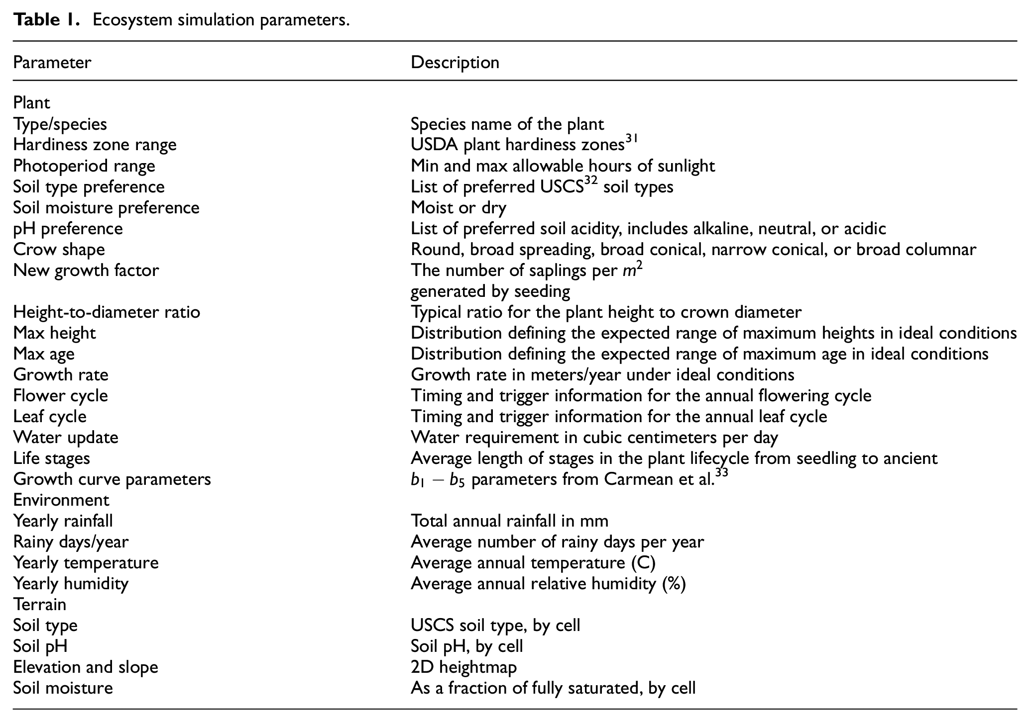
The terrain geometry is modeled as a heightmap on a regular rectangular grid. While the grid size is an adjustable parameter, a grid size of 1 m was used most often for the simulations in this work. In addition to the elevation, each cell contains information about the soil type (according to the unified soil classification system), the soil pH, and the soil moisture content.

While the terrain cell elevation, pH, and soil type are constant throughout the simulation, the soil moisture is updated dynamically using a soil evapotranspiration model similar to Singh,³⁴ as shown in Figure 1. Rainfall is added to the scene using the weather model, and evaporation is calculated using the temperature and humidity of the environment. Transpiration (uptake by each plant) is modeled as function of plant species properties and size. The soil moisture simulation uses a 2.5D accumulation approach discussed in the following section. This approach allows the two-way interaction between the soil and vegetation to dynamically modify the soil moisture content.

Figure 1.

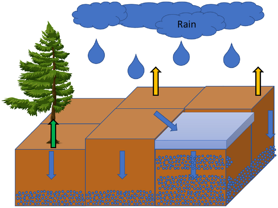
Evapotranspiration model showing the interdependence in evaporation, rain, and plant uptake in simulating soil moisture.

Plants compete with each other for both water and sunlight. Competition for sunlight manifests itself as shading—one plant obscures another from direct access to the sun. Computationally, evaluating which plants shade each other requires $n^{2}$ calculations for $n$ total plants. Since we are simulating scenes with thousands of plants, a pairwise shading calculation is not practical. Instead, the plant canopy is subdivided onto a regular two-dimensional (2D) grid as shown in Figure 2. For each plant, any cell which contains any part of that plant is considered as being occupied by that plant. In each cell, all occupying plants are compared by height, and all plants that have another taller plant in that cell are considered to be shaded in that cell. The fraction of plant cells that are shaded give the overall shading fraction for that plant. This approximation neglects important shading factors like the trees’ position relative to the sun. However, because the number of pairwise shading calculations may number in the millions, and the shading calculation must be run many thousands of times to complete a full ecosystem simulation, a more complex geometrical approach increases the computational time to an impractical degree. Therefore, the simpler fractional model was chosen for this work.

Figure 2.

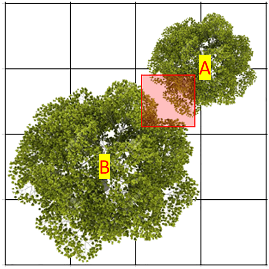
Shading calculation; the smaller tree A is 1/4 shaded by the larger tree B.

As an illustrative example of the shading calculation, consider plants A and B in Figure 2. The smaller tree, A, occupies four cells, one of which is shared by the larger tree, B. Tree A therefore has a shading fraction of 1/4, while tree B has a shading fraction of zero.

Water competition is not based on height but on root location using a similar 2D grid–based approach. A good approximation for most trees is that the root ball has the same radius as the tree crown. Each cell occupied by roots will uptake the required amount of water from the soil for that tree, as a fraction of the total occupied cells for each plant in the cell. This process repeats at each timestep as the soil moisture is either replenished by rain or depleted by root uptake and evaporation. It is noted that there are potentially other sources of soil moisture in the environment including snowmelt and runoff. While the model does not currently account for these factors, future work will incorporate these additional sources of moisture in the growth model.

Carbohydrate production and storage are used as governing metric for overall plant health in the ecosystem simulation. Plants with adequate carbohydrates will reach full growth potential. Excess carbohydrate production will result in carbohydrate storage and increased resilience to drought or other adverse phenomena. Total depletion of carbohydrates results in plant death. There are four main environmental factors in the plant growth model: shade, water, soil type, and soil pH. For each of these factors, the plant properties define the desired state of the environment for optimal plant growth and a tolerance factor quantifying the sensitivity of the plant to each factor. The growth percentage, $G_{p}$ is then given by:

G_{p} = (S_{tp} \times S) + (W_{tp} \times W) + (S L_{tp} \times SL) + (P_{tp} \times P)

(1)

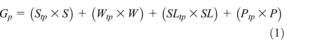
where $S_{tp}$ is the shade tolerance, $S$ is the amount of shade received, $W_{tp}$ is the water tolerance, $W$ is the amount of water received, $S L_{tp}$ is the soil tolerance, $SL$ is the suitability of the soil, $P_{tp}$ is the pH tolerance, and $P$ is the suitability of the soil pH.

Carbohydrate production is governed by the equation:

P_{p} = C_{h} \times S_{i}

(2)

where $P_{p}$ is the theoretical peak carbohydrate production, $C_{h}$ is the current plant height, and $S_{i}$ is the ideal carbohydrate production rate per height for the species.

The actual carbohydrate production $(P_{c})$ is then given by the maximum production $P_{p}$ scaled by the growth factor $G_{p}$ :

P_{c} = G_{p} \times P_{p}

(3)

4. Soil moisture model

Soil moisture is a fundamental aspect of ground vehicle simulation because it affects environmental features like vegetation growth, soil strength, and catchment formation. Here, we define a catchment as any standing body of surface water, from large puddles to permanent lakes. While there are many hydrological models that vary in scale and function, the model proposed here works mostly by taking inspiration from the process used by an established hydrological model and combining widely used formulas. These formulas and methods were selected with an emphasis on keeping runtime for simulation as low as possible without compromising accuracy. Instead of opting to emulate newer, more sophisticated hydrological models, the model of Mason et al.³⁵ was selected as the primary inspiration for the proposed model. Auxiliary functions were implemented as needed, including functions that calculate runoff and evapotranspiration, allowing our model to realistically simulate dynamic catchments that can grow, shrink, and flow. These additional functions are discussed in further detail below.

4.1. Subsurface model

In creating a generalized subsurface model, a soil moisture model separate from the catchment submodel was necessary. In effect, this model acts as a parent to the catchment submodel, handling communication between the subsurface and other models and interfacing with the catchment submodel when necessary. It uses 2D occupancy grids to store and manipulate data about soil moisture, slope, the United States Department of Agriculture (USDA) soil texture,³⁶ and vegetation density. These grids consist of square cells which correspond to coordinates in the simulated scene. However, it is important to note that the subsurface has a resolution independent from external models which allows for more control over its run time and spatial precision.

The subsurface simulation makes a few simplifying assumptions. The first assumption is that each cells soil texture can be labeled with one of the 12 USDA soil texture classes using percentage clay, silt, and loam content (ignoring organic matter). Other data such as slope and vegetation density are also separated into discrete classes. Another assumption is that water that flows off the edges of the terrain is ignored.

Wilting point is used to calculate the soil saturation at which plants will begin to wilt. In our simulation, wilting points were extracted from a table with an index for each soil texture class.³⁷ When soil gets too dry, it becomes very energy-intensive for plants to extract water from it. Therefore, the wilting point is used to determine the percent saturation at which moisture will no longer be evaporated or transpired from the cell.

Field capacity is the opposite of wilting point. It is used to determine the maximum saturation for the soil based on its soil texture. Field capacity traditionally represents the maximum volume of water soil will hold after excess water has flowed away. In our simulation, field capacity is also derived from a table based on soil type.³⁷ The proposed model assumes that between timesteps, enough water will have been run off to bring its moisture content back down to field capacity in the event that it becomes flooded or maximally saturated.

4.2. Runoff and evapotranspiration

One of the main functions of the subsurface model is to calculate runoff over a set timestep. It uses slope, precipitation amounts for each cell, vegetation densities for each cell, and runoff coefficients to calculate what amount of precipitation that is absorbed by each cell and what amount can flow onto other cells. Runoff coefficients are determined using the same method as Mahmoud et al.,³⁸ in which the ratio of water absorbed to water that will flow is determined for each cell using its vegetation density class, slope class, and USDA soil texture class. If the terrain is completely flat, all precipitation is simply absorbed until field capacity for each cell is reached.

For non-flat terrain topographies, once a cell reaches field capacity, all additional water will flow onto neighboring cells based on its slope. If the cell is also a local minimum, the subsurface model requests that the catchment submodel creates a single-cell catchment at the cell’s location. From that point on, all water that flows into that cell is added to the catchment’s volume. Before the runoff function terminates for a given timestep, it makes a request to the catchment submodel to update all catchments in the scene. This process will be explained in more detail later, but it allows the catchments to dynamically grow based on the amount of volume each one gained from the runoff function.

The other primary function of the subsurface model is to calculate evapotranspiration over a set timestep. To this end, the model uses Penman’s evapotranspiration formula for open water, bare soil, and grass.³⁹ The formula is:

E = (e_{s} - e_{d}) \times f (u)

(4)

where $E$ is the evaporated volume, $e_{s}$ is the vapor pressure at the surface, $e_{d}$ is the vapor pressure of the atmosphere, and $f (u)$ is a function for wind velocity above the surface.

To use Penman’s formula for calculating evapotranspiration, the model also uses an improved version of the Magnus formula with respect to water⁴⁰ for calculating saturated vapor pressure of water using humidity, temperature, and wind velocity. The formula is:

P_{s} = 610.94 e^{(17.625 t) / (t + 243.04)}

(5)

where $P_{s}$ is the saturated vapor pressure and $t$ is the temperature in degrees Celsius. $P_{s}$ here is the same as $e_{s}$ in Penman’s formula. This was used to calculate vapor pressure of the atmosphere using the formula:

e_{d} = e_{s} \times h

(6)

where $h$ is the percent humidity which was received as an input for the model.

An important note about Penman’s evapotranspiration formula is that the volume of water absorbed by vegetation is captured alongside the volume evaporated directly from the soil. However, the proposed subsurface model is to be separate from any model that might cause additional evapotranspiration. An example of such a scenario is the use of an external ecology model that provides transpiration values for plants growing in the soil. To deal with this, the subsurface model’s evapotranspiration function considers the water content calculated by Penman’s formula to be the minimum volume of moisture removed from each cell. The function has an input for the total requested volume of evaporated moisture from external models, which is compared with the results of Penman’s formula. For each cell, the function takes the maximum between the volume calculated by Penman’s model and the requested volume from external models, removing the resulting volume from the cell as evapotranspiration.

4.3. Catchments

To accurately model soil moisture, there was also a need to model bodies of water that might form in a generated scene. This is a key aspect of the subsurface model that sets it apart from traditionally used soil moisture models. The model uses loops and nested conditional statements to capture realistic behavior of catchments. This resulted in the creation of a separate submodel for managing bodies of water.

Based on changes in catchment volume between timesteps, catchments might grow, shrink, flow into one another, dry up, merge, or split. Using cell heights and saturation properties as provided by the subsurface model, the catchment submodel can capture all these events. This is done using a recursive update function which updates each catchment in the model based on its change in volume until equilibrium has been achieved.

Once a cell which is located at a local minimum on the terrain surpasses field capacity, the subsurface model makes a request to the catchment submodel to create a catchment at that location. This updates 2D occupancy grids which save information on which catchment each cell belongs to. It then determines at what volume the catchment will dry up and at what volume the catchment will grow. These volumes are calculated based on the height of the highest submerged cell in the catchment and the lowest neighboring unsubmerged cell. They are stored in a catchment class and added to the catchment submodel’s list of catchments. Excess water is added to the cells’ initial volume.

Catchments are deleted when they dry up. When the subsurface model’s evapotranspiration function removes more moisture from a catchment than it has in remaining volume, it makes a request to the catchment submodel to delete the catchment. During its execution, the remaining negative balance of moisture is removed from each cell in the catchment by an equal percentage of each cell’s maximum soil moisture (field capacity). The catchment submodel’s occupancy grids are also updated to reflect these changes.

One notable assumption made by the catchment submodel is that any catchment that contains cells on the edge of the map is assumed to be large enough to no longer require processing by the update function. To capture this effect, all catchment classes in the submodels’ catchment list have a Boolean variable that determines whether it is “dynamic.” This allows external models to control whether each catchment should be able to change shape or not. In the catchment submodels update function, before calculations for growth and shrinkage are executed, each catchment is checked to make sure it is dynamic.

In the update function, each dynamic catchment in the model is checked to see if either its volume exceeds the volume at which the catchment should grow or if its volume falls below the volume at which the catchment should shrink. These volumes are recalculated in the same way as is described earlier.

Sometimes catchments will need to interact with one another. In the update function, there are times when a catchment will exceed the volume at which it needs to grow but will be unable to do so in the way explained above. If the catchment’s lowest neighboring cell is inside of another catchment, it means that it must either flow into the other catchment or merge with the other catchment. To determine which of the two must take place, the function checks the status of the other catchment.

For clarity, let us refer to the original catchment as $C_{1}$ and the other catchment as $C_{2}$ . If $C_{2}$ ’s lowest neighboring cell is inside of $C_{1}$ , the update function removes $C_{2}$ from the table, adds its volume to that of $C_{1}$ and adds all of its cells to $C_{1}$ . This effectively merges the two catchments as demonstrated in Figure 3.

Figure 3.

Sometimes, when a catchment exceeds its growth volume, its lowest neighboring catchment will already belong to another catchment. If both the catchment and the neighboring catchment are flowing into one another, the two catchments are merged.

If this conditional statement fails, $C_{1}$ merely flows into $C_{2}$ , as $C_{2}$ is not yet large enough for the two catchments to be merged. This is done by adding the extra volume from $C_{1}$ to the volume of $C_{2}$ . This process is illustrated in Figure 4. At this point, the update function quits and restarts to make sure that $C_{2}$ can be updated with its new volume.

Figure 4.

If the neighboring catchment is not also flowing into the original catchment, the original catchment will flow into the other catchment.

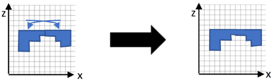
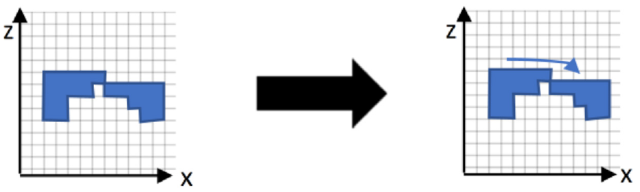
If a catchment shrinks and, as a result, has been separated into two or more separate bodies of water, the update function must split the catchment. This is done using Breadth-First Search (BFS). When a catchment with three or more cells shrinks, BFS is executed on one of the removed cells submerged neighbor cells. All cells in the catchment that are connected to this neighboring cell are removed from the original catchment and added to a new catchment. After the BFS terminates, if there are any remaining cells that have not been removed from the original catchment, it means that the catchment has split. BFS is then executed again on another of the removed cells neighbors, and the process is repeated until all cells in the original catchment are accounted for. This process is demonstrated in Figure 5.

Figure 5.

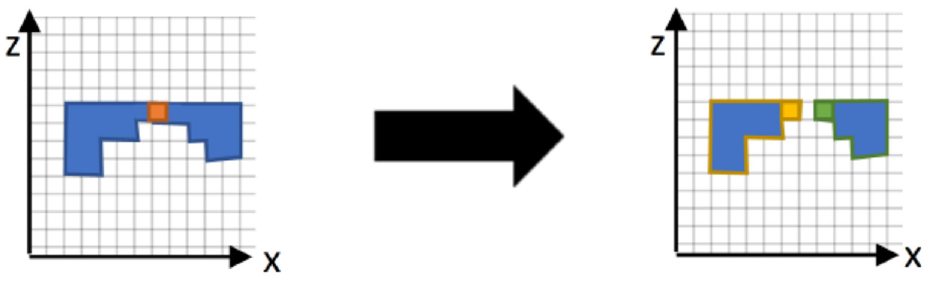
When a cell is removed from a catchment with three or more cells, BFS is executed on its neighboring cells to handle any splitting of the catchment. In this figure, the red cell was removed, and two new catchments were created by running BFS on the yellow and green neighboring cells.

5. Results

This section shows results from the ecosystem simulations for two applications. We show some high-fidelity renderings of terrains generated using the ecosystem simulator, along with lidar scans of the same scenes. In the mobility experiments, we demonstrate how the distribution of trunk diameters from our method is more realistic than competition-only models and show how this result can influence AGV mobility.

5.1. Example scenes

The ecosystem simulation described above outputs the size, location, and species of plants over a given terrain. It does not include any information about mesh geometry or attributions. Therefore, to render the scenes, it is necessary to create meshes associated with each item of vegetation in the ecosystem simulation output. In this work, we use plant models purchased from Xfrog⁴¹ as instantiations of the mesh geometries. Each species represented in the simulation output has an associated mesh file. For trees, this includes separate geometries for the young, medium, and adult life stages of the tree.

The geometric models are scaled according the height and trunk diameter output by the ecosystem simulation and placed into the scene at the locations output by the simulator. The tree models are rotated by a random amount about the vertical axis of the scene so that all the meshes are not aligned. The scenes are then rendered using the MSU Autonomous Vehicle Simulator (MAVS),⁴² an open-source simulator for AGV that includes various sensor and environment models. The results of these renderings are shown in Figure 6.

Figure 6.

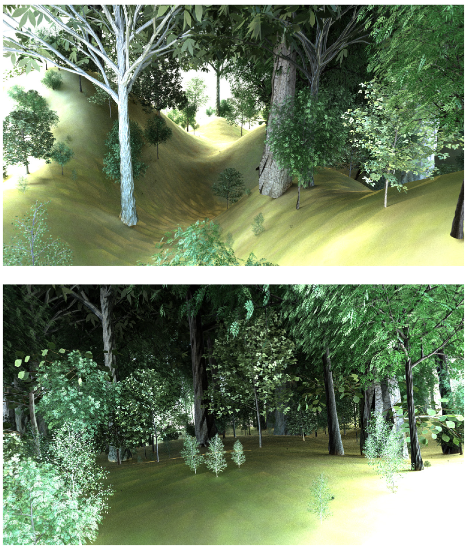
Rendering of two ecosystems created with the method described in this paper: (top) a medium-density forest on hilly terrain; (bottom) a young forest with a lower basal area and more undergrowth.

MAVS can also simulate many common terrestrial lidar models and has been shown to yield accurate results for lidar interacting with vegetation.¹⁹ In order to demonstrate the ability of our ecosystem to support AGV simulations, example output from synthetic lidar scans in the scenes generated with our ecosystem simulator is shown in Figure 7 for three different lidar models—Velodyne VLP-16 (top), HDL-32E (middle), and Ouster OS1-64 (bottom). Figure 7 shows the same forest and sensor position as the bottom image in Figure 6.

Figure 7.

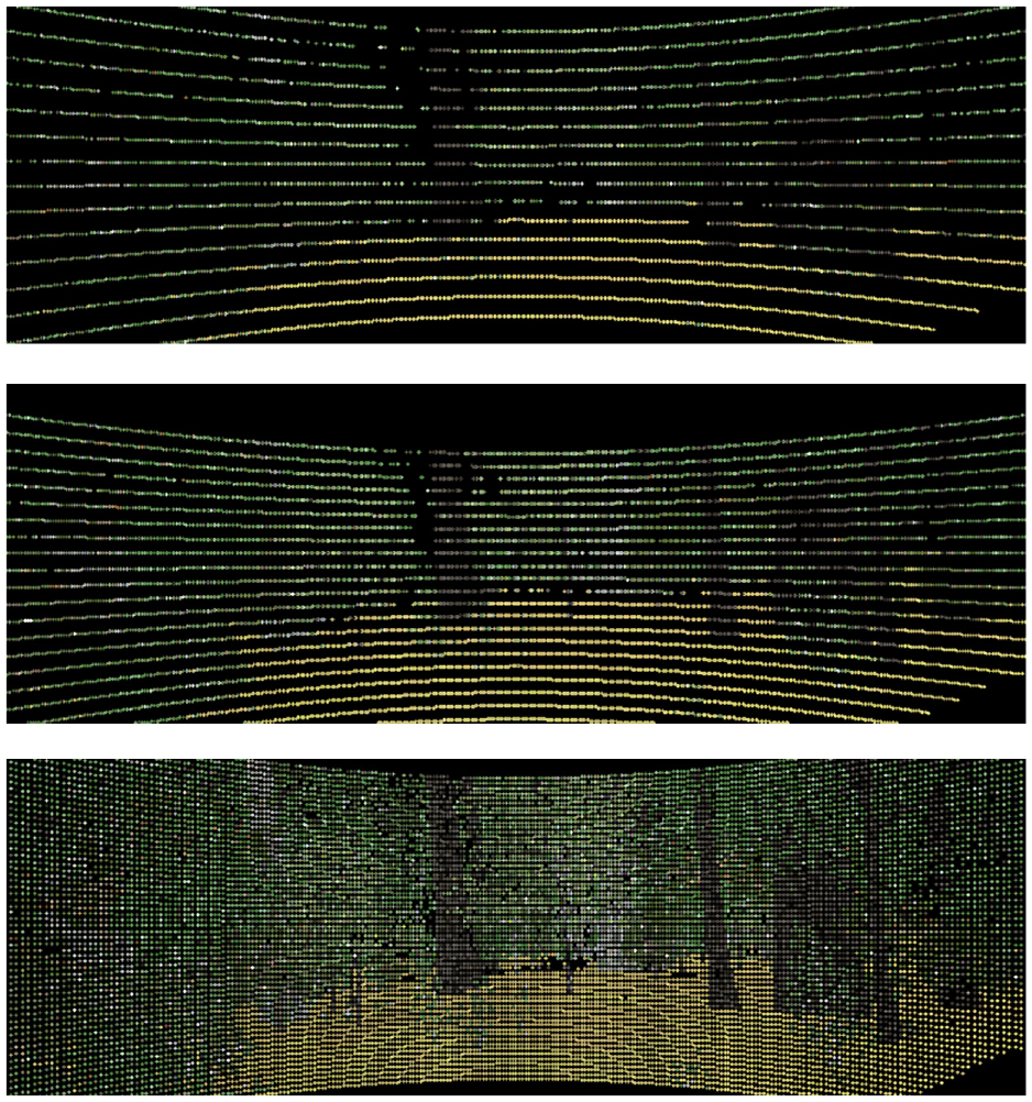
Colorized lidar scan of the forest ecosystem created with the method in this paper for a Velodyne VLP-16 (top), HDL-32E (middle), and Ouster OS1-64 (bottom).

5.2. Analysis of mobility through vegetation

In this section, we show the results of our ecosystem simulation in terms of distribution of trunk/stem diameters and demonstrate the significant influence this distribution has on AGV mobility. The simulated scenes generated in this section shown in Figures 8 and 9 were broadleaf, deciduous forests in a humid subtropical climate. The tree species included horse chestnut, birch, pecan, and magnolia. The yearly rainfall rate was about 62 inches per year, and the soil type was silt. The ecosystems were allowed to grow until they reached a desired basal area (BA), which is the total cross-sectional area of all the stems at breast-height per unit area of land, typically per acre.⁴³

Figure 8.

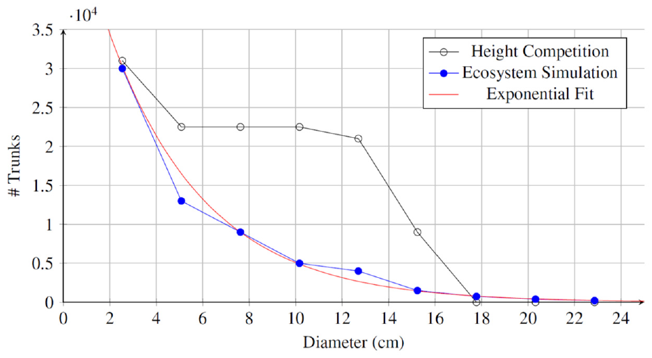
Distribution of trunk sizes for ecosystem simulation.

Figure 9.

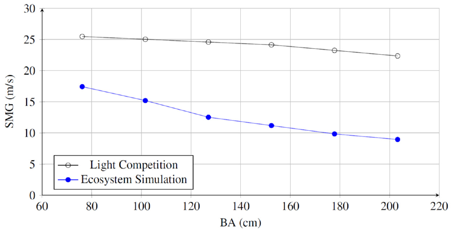
Speed made good versus BA for different light competition only (black) and our ecosystem simulation (blue) procedural generation.

Figure 8 shows the results of two different types of ecosystem simulations. The black open circles show the results of the light-only competition model similar to that implemented in Deussen et al.,²⁴ while the blue dots show the result of our simulation. Both simulations were run until the total plant density reached a BA of 50, which represents a medium-density forest.

In Figure 8, it is clear that the two ecosystem simulations give noticeably different results for the trunk diameter distribution. The light-only model results in an over abundance of small and medium diameter trees and an under-abundance of large diameter trees. In contrast, the ecosystem simulation approach presented in this work results in an exponential distribution of tree diameters. This type of negative exponential distribution for tree trunk diameters is notably well known in the forestry literature.⁴⁴ We will show that the difference in the two distributions shown in Figure 8 results in important differences in the expected mobility of AGV through the vegetation.

Next, a demonstration of the influence that the ecosystem simulation has on the mobility of the vehicle is presented. In order to achieve this, the ecosystems created by our simulation are used as inputs into a mobility analysis with the NATO Reference Mobility Model (NRMM), a ground vehicle mobility analysis tool that has been used for several decades to support the design and acquisition of military vehicles by the United States Army and other NATO nations.⁴⁵ The NRMM uses vehicle characteristics like gross vehicle weight, tire size and shape, and tractive force versus speed (a measure of the overall power of the vehicle) to predict the mobility performance through off-road terrain. Terrain properties include slope, roughness, soil type, and vegetation density. Vegetation is accounted for in two ways in the NRMM—as the time it takes to avoid large vegetation and the time it takes to override smaller vegetation. Therefore, the overall cross-country mobility prediction made by NRMM is sensitive to both the size and distribution of the vegetation in the environment. For this reason, NRMM mobility predictions prove to be an important discriminator for the importance of vegetation distribution in a scene.

Vegetation override—the ability of a vehicle to push through vegetation—is an important aspect of AGV mobility. Empirical models for the force imparted on a vehicle by a cluster of vegetation have been implemented in the NRMM using the following formula:⁴⁶

F_{vi + 1} = 12 w_{v} 100 \sum_{j = 1}^{i} d_{j} d_{vi}^{3}

(7)

where $F_{vi + 1}$ is the average force to override vegetation $\leq class$ $i$ , $w_{v}$ is the vehicle width in inches, $d_{j}$ is the vegetation stem density for each class (1/in²), and $d_{vi}$ is the average stem diameter in class $i$ (inches). In this formula, individual plants are sorted into classes according to their trunk/stem diameter. The stem density for class $i$ is given by $d_{i}$ :

d_{i} = \frac{4}{π} [\frac{1}{s_{i}^{2}} - \frac{1}{s_{i + 1}^{2}}], i = 1, . . ., N_{i} - 1

(8)

where $d_{i}$ is the density of stems in stem diameter class i in $(\frac{1}{i n^{2}})$ , $s_{i}$ is the average spacing of stems in class $i, i + 1, . . . N_{i}$ (inches), and $N_{i}$ is the number of stem diameter classes.

Using vehicle characteristics like the tractive force versus speed curve, NRMM can make predictions like speed-made-good (SMG) for a terrain with a certain vegetation distribution using Equations (7) and (8). In our analysis, we compared the SMG for a Polaris MRZR overriding vegetation in forests with different BAs using two types of distributions—those generated with light competition only and those generated with our ecosystem model. Figure 9 shows the results of this analysis. In this figure, the black dots represent the SMG results when using traditional light competition-only vegetation distributions, while the blue dots show the results when using the vegetation distribution generated using the method from this paper.

Overall, the SMG is much lower for the exponential vegetation distributions generated by our ecosystem simulator. This is due to the cubic dependence on diameter in Equation (7) for override force. Even a small number of larger diameter trees results in a much higher average override force, and hence a lower overall SMG. In addition, Figure 9 shows that increasing overall BA has more of an impact when using distributions generated by our model than when using traditional gaming-style flat distributions. The primary conclusion from this mobility analysis can therefore be summarized in two statements. First, the ecosystem simulation proposed in this work yields a more realistic size distribution for vegetation than previous gaming-based approaches (Figure 8). Second, NRMM analysis reveals that this size distribution is critically important in predicting vehicle mobility through vegetation (Figure 9), primarily due to the vehicles ability to either override or avoid the vegetation based on its size.

We note that 50 different scenes were generated for each BA, and the results shown in Figure 9 are the average of all the results. More detail on NRMM and SMG calculations as a function of vegetation size distribution can be found in Hudson.⁴⁷

6. Summary and conclusions

In this work, we have presented a new method for ecosystem simulation for the purpose of developing synthetic off-road terrains. Our method couples together groundwater, surface water, soil and weather conditions, and vegetation growth and competition processes to create a realistic feedback loop between terrain and vegetation that produces a natural looking scene that also follows well-known size distributions for vegetation stem/trunk diameter. Our NRMM analysis showed that:

Our method yields a more realistic vegetation size distribution that randomized approaches.

This distribution is critical in predicting vehicle mobility in off-road environments.

Planned future work in this area will include incorporation of user-defined terrain features like roadways, bridges, ditches, rivers, or ponds into the growth model. In addition, the soil moisture model will be updated to include sources other than rain such as snowmelt and runoff.

Footnotes

Funding

The research described and the resulting data presented herein, unless otherwise noted, was funded under PE 0602784A, Project T53 “Military Engineering Applied Research,” Task 11.3 under Contract No. W56HZV-17-C-0095, managed by the US Army Combat Capabilities Development Command (CCDC) and the Engineer Research and Development Center (ERDC). The work described in this document was conducted at the Center for Advanced Vehicular Systems, Mississippi State University. Permission was granted by ERDC to publish this information. DISTRIBUTION A. Approved for public release; distribution unlimited.

ORCID iD

Christopher Goodin

Author biographies

Christopher R Hudson is a Research Engineer for the Advanced Vehicle Systems group at the Center for Advanced Vehicular Systems at Mississippi State University. Dr Hudson earned his BS in Computer Science in 2014 from the Department of Mathematics and Computer Science at the University of North Carolina at Pembroke. In 2022, Dr Hudson earned his PhD from the Department of Computer Science and Engineering at Mississippi State University. Dr Hudson works on a variety of projects focusing on off-road autonomous systems. This works explores both modeling and simulation combined with real-world testing and validation. His dissertation focused on the effects of ecological simulation for ground vehicle mobility forecasting. Dr Hudson’s work extends into Virtual Reality, with a focus on designing interactions in dynamic environments to explore human–computer interactions in complex scenarios in a safe and controlled manner. This work involves interactions with and around autonomous systems and immersive training for controlling remote systems.

Warren Wheeler is currently an Associate Software Engineer at Quantifind. He graduated from Mississippi State University with an MS in Computer Science in 2022.

Christopher Goodin is an Associate Research Professor at the Mississippi State University Center for Advanced Vehicular Systems (CAVS). He received his BS in mathematics and physics from Mississippi College in 2004 and PhD in physics from Vanderbilt University in 2008. From 2008 to 2017, he worked with the US Army Engineer Research and Development Center (ERDC) in Vicksburg, MS, developing physics-based simulations of ground vehicles, sensors, and robotics and serving as the lead developer for the Virtual Autonomous Navigation Environment (VANE) and the Computational Research and Engineering Acquisition Tools and Environments for Ground Vehicles (CREATE-GV). At CAVS, Dr Goodin is the lead developer of the MSU Autonomous Vehicle Simulator (MAVS), a simulation library for autonomous ground vehicles, and the NATURE off-road autonomy software stack.

Daniel W Carruth is Associate Director for Advanced Vehicle Systems at the Center for Advanced Vehicular Systems and an Associate Research Professor at Mississippi State University. Dr Carruth earned his BS in Computer Science and Engineering in 2001 and his PhD from the Department of Psychology at Mississippi State University in 2008. Dr Carruth contributes to NATO Applied Vehicle Technology Panel research task groups (AVT-327 and AVT-341) focused on modeling and simulation of military ground vehicles. He is a member of SAE and ASAM. He has published over 100 conference proceedings and articles in journals such as Sensors, Electronics, Transportation Safety & Security, International Journal of Social Robotics, and International Journal of Industrial Ergonomics.

Nicholas Harvel is a Graduate Assistant at CAVS and PhD Candidate in Computer Science. He received his MS in Computer Science in 2024.

Joshua Ferguson is a software developer. He graduated from Mississippi State University with a MS in Computer Science in 2022.

J. Gabriel Monroe graduated from Mississippi State University (MSU), earning both his BS (2012) and PhD (2016) degrees in Mechanical Engineering. Since graduating, he has worked as a Research Mechanical Engineer at the US Army Engineer Research and Development Center (ERDC). His primary research involves the modeling and simulation of manned and unmanned mobility systems, with a particular focus on scene generation and software-in-the-loop simulations for autonomous systems development.

David P McInnis graduated from Mississippi State University (MSU), earning both his BS (2010) and MS (2017) degrees in Mechanical Engineering. Since graduating, he has worked as a Research Mechanical Engineer at the US Army Engineer Research and Development Center (ERDC). His primary research involves the modeling and simulation of manned and unmanned mobility systems, having led research teams to simulate leader follower vehicle systems. His particular focus is on scene generation and environmental conditions modeling for software-in-the-loop simulations for autonomous systems development.

References

Kelly

Stentz

Amidi

, et al. Toward reliable off road autonomous vehicles operating in challenging environments. Int J Robot Res 2006; 25: 449–483.

Fadaie

. The state of modeling, simulation, and data utilization within industry: an autonomous vehicles perspective. [preprint] arXiv 2019. DOI: 10.48550/arXiv.1910.06075.

Milford

Anthony

Scheirer

. Self-driving vehicles: key technical challenges and progress off the road. IEEE Potent 2019; 39: 37–45.

Papadakis

. Terrain traversability analysis methods for unmanned ground vehicles: a survey. Eng Appl Artif Intell 2013; 26: 1373–1385.

Goodin

Dabbiru

Hudson

, et al. Fast terrain traversability estimation with terrestrial lidar in off-road autonomous navigation. In: Unmanned systems technology XXIII, Orlando, FL, SPIE-DCS 2021, Vol. 11758, pp 189–199. Bellingham, WA:International Society for Optics and Photonics.

Maturana

Chou

Uenoyama

, et al. Real-time semantic mapping for autonomous off-road navigation. In: Hutter

Siegwart

(eds) Field and service robotics. London: Springer, pp. 335–350.

Dabbiru

Goodin

Scherrer

, et al. Lidar data segmentation in off-road environment using convolutional neural networks (CNN). SAE Int J Adv Curr Pract Mobil 2020; 2: 3288–3292.

Goodin

Carruth

Dabbiru

, et al. Simulation-based testing of autonomous ground vehicles. In: Autonomous systems: sensors, processing and security for ground, air, sea and space vehicles and infrastructure, Orlando, FL, 3–7 April 2022, pp. 167–174. Bellingham, WA: SPIE.

Dosovitskiy

Ros

Codevilla

, et al. Carla: an open urban driving simulator. [preprint] arXiv 2017. DOI: 10.48550/arXiv.1711.03938

10.

Macedo

Manduchi

Matthies

. Ladar-based discrimination of grass from obstacles for autonomous navigation. In Rus

Singh

(eds) Experimental roboticsVII. Berlin: Springer, 2001, pp. 111–120.

11.

Bradley

Unnikrishnan

Bagnell

. Vegetation detection for driving in complex environments. In: 2007 IEEE international conference on robotics and automation (ICRA), Rome, Italy, 2007, pp. 503–508, New York: IEEE.

12.

Foroutan

Tian

Goodin

. Assessing impact of understory vegetation density on solid obstacle detection for off-road autonomous ground vehicles. ASME Letters Dyn Sys Control 2020; 1: 021008.

13.

Goodwin

Coops

Culvenor

. Development of a simulation model to predict lidar interception in forested environments. Remote Sens Environ 2007; 111: 481–492.

14.

Sun

Ranson

. Modeling lidar returns from forest canopies. IEEE Trans Geosci Remote Sens 2000; 38: 2617–2626.

15.

Hovi

Korpela

. Real and simulated waveform recording lidar data in juvenile boreal forest vegetation. Remote Sens Environ 2014; 140: 665–678.

16.

Deschaud

Prasser

Dias

, et al. Automatic data driven vegetation modeling for lidar simulation. In: IEEE international conference robotics and automation (ICRA), St. Paul, MN, 14–18 May 2012, pp. 5030–5036. New Jersey: IEEE.

17.

Browning

Deschaud

Prasser

, et al. 3D mapping for high-fidelity unmanned ground vehicle lidar simulation. Int J Robot Res 2012; 31: 1349–1376.

18.

Goodin

Gates

Cummins

, et al. High-fidelity physics-based simulation of a UGV reconnaissance mission in a complex urban environment. In Unmanned Systems Technology XIII, Orlando, Florida, SPIE DCS 2011, Vol. 8045.

19.

Goodin

Doude

Hudson

, et al. Enabling off-road autonomous navigation-simulation of lidar in dense vegetation. Electronics 2018; 7: 154.

20.

Bossel

. Treedyn3 forest simulation model. Ecol Modell 1996; 90: 187–227.

21.

Peng

. Growth and yield models for uneven-aged stands: past, present and future. For Ecol Manag 2000; 132: 259–279.

22.

Weiskittel

Hann

Kershaw

Jr , et al. Forest growth and yield modeling. Hoboken, NJ: John Wiley & Sons, 2011.

23.

Firbank

Watkinson

. A model of interference within plant monocultures. J Theor Biol 1985; 116: 291–311.

24.

Deussen

Hanrahan

Lintermann

, et al. Realistic modeling and rendering of plant ecosystems. In: Proceedings of the 25th annual conference on computer graphics and interactive techniques, Las Vegas, NV, 22–24 July 1998, pp. 275–286, New York: ACM.

25.

Lane

Prusinkiewicz

. Generating spatial distributions for multilevel models of plant communities. In: Graphics interface, Vol. 2002, Calgary, AB, Canada, 27−29 May 2002, pp. 69–87. Citeseer.: Canadian Human-Computer Communications Society (CHCCS)

26.

Hendrikx

Meijer

Van Der Velden

, et al. Procedural content generation for games: a survey. ACM Trans Multimed Comput Commun Appl 2013; 9: 1–22.

27.

Prusinkiewicz

Mündermann

Karwowski

, et al. The use of positional information in the modeling of plants. In: Proceedings of the 28th annual conference on computer graphics and interactive techniques, Los Angeles, CA, 12–17 August 2001, pp. 289–300. New York: ACM.

28.

Kim

Cho

. Efficient modeling of numerous trees by introducing growth volume for real-time virtual ecosystems. Comput Animat Virt Worlds 2012; 23: 155–165.

29.

Beneš

Andrysco

Št’ava

. Interactive modeling of virtual ecosystems. In: Galin

Schneider

(eds) Proceedings of the fifth Eurographics conference on natural phenomena, Goslar: Eurographics Association, 2009, pp. 9–16.

30.

Cordonnier

Galin

Gain

, et al. Authoring landscapes by combining ecosystem and terrain erosion simulation. ACM Trans Graph 2017; 36: 1–12.

31.

Cathey

. USDA plant hardiness zone map, Vol 1475. Washington, DC: US Department of Agriculture, 1990.

32.

García-Gaines

Frankenstein

. USCS and the USDA soil classification system: development of a mapping scheme. Technical Report ERDC-CRREL TR-15-4, 1 March 2015. Vicksburg, MS: US army engineer research and development center.

33.

Carmean

Hahn

Jacobs

, et al. Site index curves for forest tree species in the eastern United States. Technical Report NC-128, Washington, DC: USDA Forest Service, 1989.

34.

Singh

. Hydrologic systems. Vol. I. Rainfall-runoff Modeling. Englewood Cliffs, NJ: Prentice Hall, 1988.

35.

Mason

Ahlvin

Green

. Short-term operational forecasts of trafficability. Technical Report 20020510-83, 1 October 2001. Vicksburg, MS: US army engineer research and development center.

36.

United States Department of Agriculture. Soil mechanics level 1 Module 3 USDA textural classification. Washington, DC: USDA Soil Conservation Service, 1987.

37.

Gupta

Papritz

Lehmann

, et al. GSHP: Global database of soil hydraulic properties. Technical report, soil and terrestrial environmental physics, department of environmental systems science, 2021.

38.

Mahmoud

Alazba

. Hydrological response to land cover changes and human activities in arid regions using a geographic information system and remote sensing. PLoS ONE 2015; 10: e0125805.

39.

Penman

. Natural evaporation from open water, bare soil and grass. Proc R Soc Lon A Math Phys Sci 1948; 193: 120–145.

40.

Huang

. A simple accurate formula for calculating saturation vapor pressure of water and ice. J Appl Meteorol Climatol 2018; 57: 1265–1272.

41.

Henke

Kniemeyer

Kurth

. Realization and extension of the Xfrog approach for plant modelling in the graph-grammar based language XL. Comput Inform 2017; 36: 33–54.

42.

Hudson

Goodin

Miller

, et al. Mississippi state university autonomous vehicle simulation library. In: Proceedings of the ground vehicle systems engineering and technology symposium, Novi, MI, 11–13 August 2020, pp. 11–13.

43.

West

. Use of diameter increment and basal area increment in tree growth studies. Can J For Res 1980; 10: 71–77.

44.

Rubin

Manion

Faber-Langendoen

. Diameter distributions and structural sustainability in forests. For Ecol Manag 2006; 222: 427–438.

45.

Petrick

Janosi

Haley

. The use of the NATO reference mobility model in military vehicle procurement. SAE Technical Paper 810373, 1 February 1981.

46.

Haley

Jurkat

Brady

. NATO reference mobility model, Edition 1. Vol. 2. Users guide, Obstacle module. Technical Report 12503, Hoboken, NJ: Highly Filled Materials Inst, Stevens Inst of Technology, 1979.

47.

Hudson

. The effects of ecological simulation for ground vehicle mobility forecasting. Mississippi State University, 2022.