
Abstract
The growing intricacy of contemporary engineering systems, typically reduced to differential equations, poses a difficulty in digitally simulating them. The linearly implicit quantized state system (LIQSS) provides a different method from traditional numerical integration techniques for tackling such problems. This method is effective in large sparse stiff systems and systems with frequent discontinuities. However, this method could be further improved. First, the algorithm can step through the solution analytically or through iterations. A comparison is presented in this article. Second, the intrinsic discrete behavior of this new method can cause oscillations that lead to small unnecessary simulation steps. A prior approach was made to detect and terminate these cycles. Different detection mechanisms are examined in this article. Third, a linear approximation was used. Its enhancement is also investigated in this work. Finally, the article provides which of these modifications improved the overall performance of some systems simulations using LIQSS order one.
1. Introduction
The modeling of complex engineering systems is often reduced to differential equations that exhibit stiffness and frequent discontinuities. Stiffness and discontinuities can be a challenge in the numerical integration of such equations by classic methods. 1
Depending on the nature of the problem, traditional solvers use explicit and implicit methods. While explicit methods are cheaper, they perform poorly in the face of stiff problems, because maintaining computational stability requires a step size reduction. This increases computational cost and can make simulations impractical or even infeasible for large-scale systems. 2 Traditional solvers resort to implicit techniques that also involve costly iterations and matrix inversions, with an expense that grows proportionally to the size of the system. 3
Quantized state system (QSS) methods are explicit and linearly implicit algorithms that aim to handle these issues more efficiently. They replace the classic time-slicing methods with a quantization of the states, leading to an asynchronous discrete-event simulation model. QSS algorithms are asynchronous because system variables do not necessarily get updated at the same time.4,5 Solving some stiff differential equations using the linearly implicit quantized state system (LIQSS) can produce oscillations that lead to unnecessary steps. A modification was proposed to handle this issue, and a modified solver (mLIQSS) was developed and tested by Di Pietro et al. 6
In this article, further modifications that aim to enhance the step size, the cycle detection, and the existing linear approximation, are proposed. In addition, the simulation results of these modifications are compared. The paper is organized as follows: Section 2 presents the background concepts of QSS and mLIQSS. Section 3 explains the modifications of the step size, the detection mechanism, and the linear coefficients. In section 4, the results of the modifications in the Tyson model and the advection-diffusion reaction problem are presented. Finally, section 5 concludes the article.
2. Background
2.1. QSS
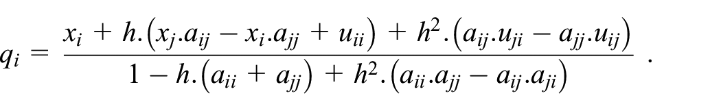
QSS methods, including LIQSS, are alternatives to traditional integration methods for solving ordinary differential equations (ODEs). These methods are specially designed to solve challenges posed by the increasing complexity of modern systems. The main idea behind QSS methods is to divide the system state space into quantized regions and represent the system state in terms of these quantized values. The QSS methods update the system status only when certain thresholds or conditions are met, instead of continuously simulating the system’s behavior. These methods offer advantages such as reduced computational cost and improved performance compared with traditional numerical integration methods. In solving the following system of

where

where
QSS methods were shown to have nice stability and error-bound properties 8 while also outperforming some classic solvers.3,9
2.2. mLIQSS
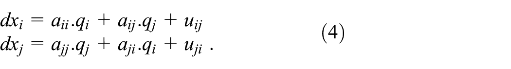
In LIQSS, all steps involve single variable updates depending on the future direction of

where
where
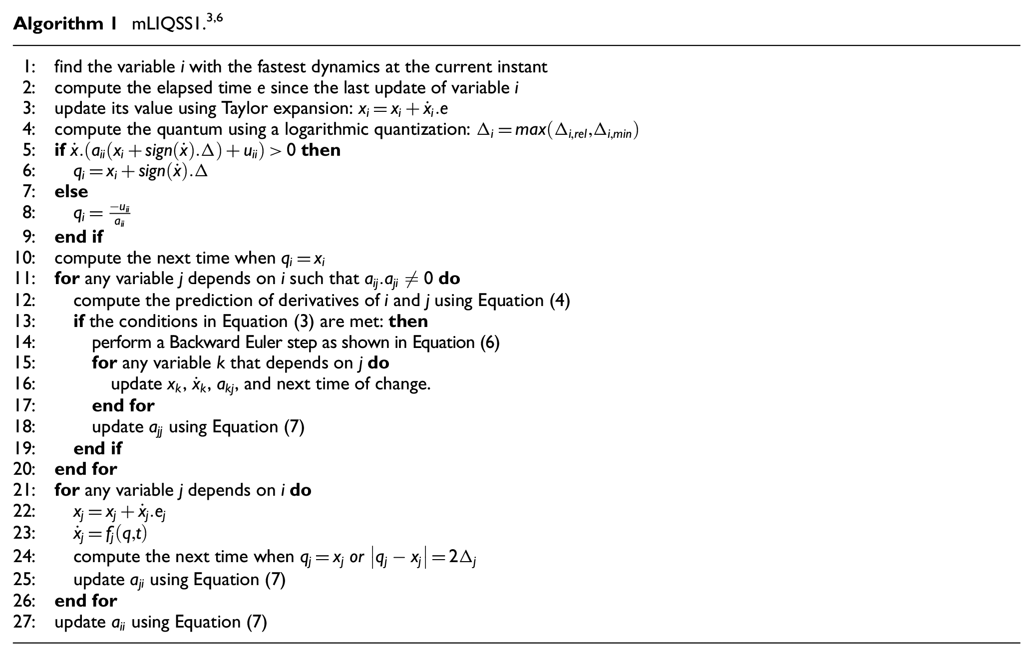
A modification to the original LIQSS algorithm was implemented in Algorithm 1.
When a cycle is detected, a simultaneous update must occur. In order to simultaneously update
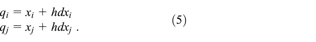
Using Equations (5) and (4) is equivalent to performing a Backward Euler step. This is formulated as follows:
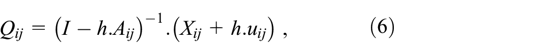
where
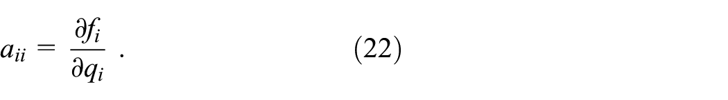
The linear approximation coefficients are updated as follows:
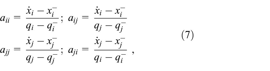
where
The value of

where
2.3. Iteration and analytic approaches
Di Pietro et al.
6
stated that the calculation of
2.3.1. Single update
Besides the analytic approach shown in Algorithm 1, Equation (9) can be used to solve for

where
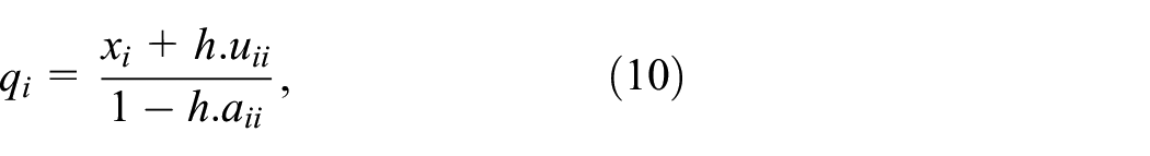
The value
where
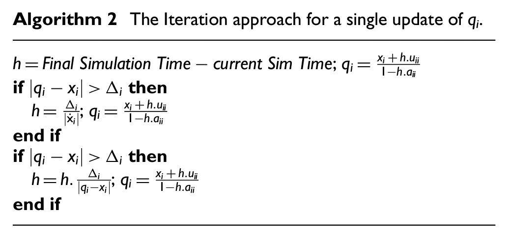
Algorithm 2 describes the iteration approach. The algorithm starts by guessing an
The Iteration approach for a single update of q i .
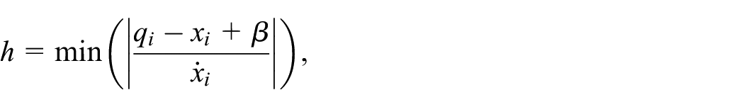
A different explanation of the analytic approach uses Equation (10). Adding and subtracting
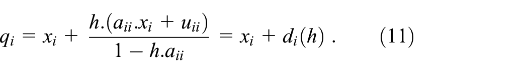
For the analytic method, in order to maximize
Distance
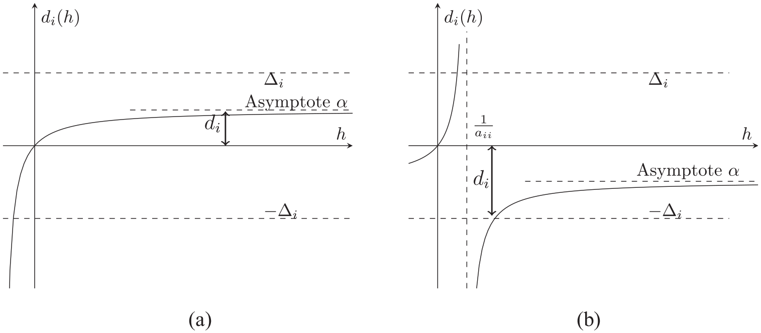
The analytic approach is described in Algorithm 3. At most, the algorithm checks three inequalities. This analytic method is similar to the one presented in lines (5-9) of Algorithm 1. However, it uses a different explanation that can be easily extended to higher orders, and it does not rely on the conditions of checking the signs of the derivatives.
The Analytic approach for a single update.
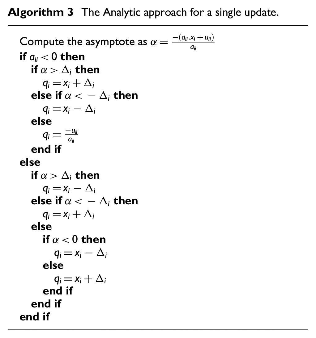
Using the function
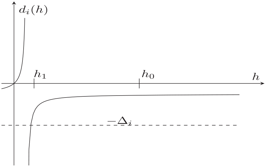
Drawbacks of the iteration approach in a single update.
2.3.2. Simultaneous update
Similar to the single update, analytic and iteration methods are introduced for the simultaneous update. To investigate the difference between them, Equation (6) is expanded. The first row leads to the following:
Adding and subtracting

where
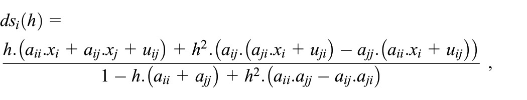
is the distance between
Similarly, the second row leads to

where
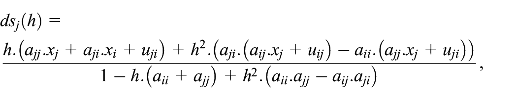
is the distance between
Algorithm 4 describes the iteration approach in the simultaneous update. The algorithm starts by guessing an
The Iteration approach in the simultaneous update order 1.

For the analytic method, in order to maximize
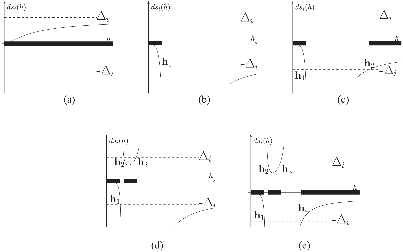
Different positions of the quantum
The equations
Let us use
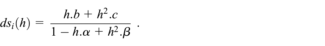
Let us start by
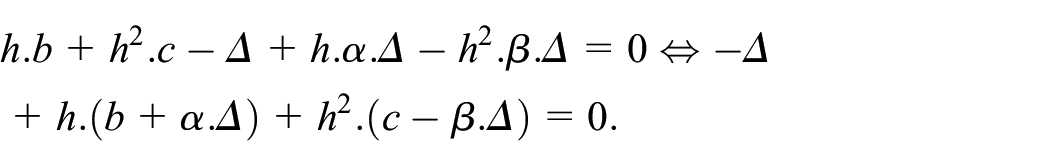
This last equation can have 2 real roots. Similarly,
Based on the number of roots, acceptable intervals (
Similarly, acceptable intervals for variable
The analytic approach in the simultaneous update order 1.
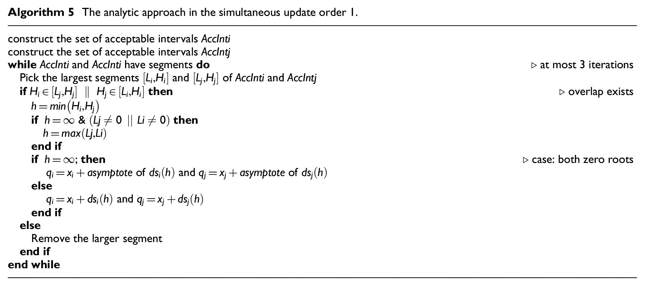
A search for the largest overlap between
3. Modifications
This section presents two possible modifications to the current mLIQSS algorithm. First, different conditions to predict cycles are investigated. Second, a different approach to updating the linear coefficients is introduced.
3.1. Cycle detection mechanism
The fundamental concept of the QSS method revolves around the cheap update of a single variable. However, such an update can trigger sudden shifts in other variables, resulting in shorter steps. The reduction of the step count caused by a simultaneous update within a trajectory is a sign of the presence of a cycle. Yet, practically this criterion cannot be directly exploited as we lack the forthcoming step count. Hence, each step necessitates a judicious decision. Currently, order 1 cycle detection relies on the change of both derivatives’ signs as shown in Equation (3). These criteria may miss cycles in some cases.
First, consider the case shown in Figure 4. This situation contains cycles, but at every step, only one variable changes direction. At
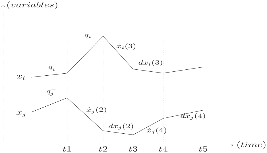
Using the change of the derivatives’ signs in cycle detection.
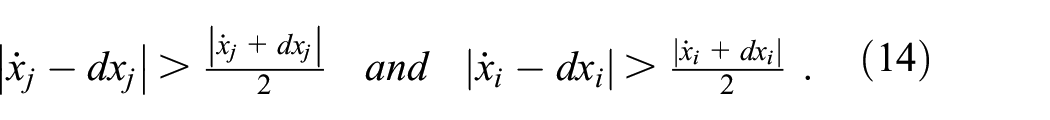
Second, consider the case shown in Figure 5. At
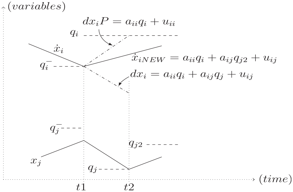
Comparing
Therefore, Equation (15) can also be used for cycle detection:

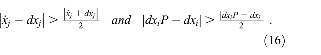
Finally, both former cases can be considered as shown in Equation (16):
3.2. More accurate linear coefficients
For accurate identification of cycles and optimal step sizes, the prediction of future derivatives through a linear approximation must be highly precise. Erroneous values could force the step size to be small, miss cycles, or conduct unnecessary expensive simultaneous updates, which could hurt the overall performance. Therefore, the coefficients of the linear approximation

where
First, the method used in Equation (7) is not accurate in case of a simultaneous update of


Another variable

Subtracting Equation (20) from Equation (19) leads to the expression that finds
Second, in large nonlinear systems where the coefficient

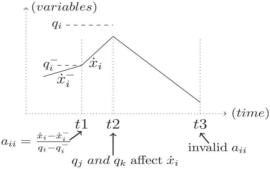
At the end of the step at time
The article investigates another possible way to approximate the derivative function using the Jacobian entries of the original derivative function as coefficients of the linearization
Hence,
Going back to the example in Equation (21), the coefficient
Computing the original Jacobian entries of the system can be better and cheaper than finding the coefficients manually, as finding these values costs one function call. This approach extracts the Jacobian entries as expressions in a function during compilation time. Hence, this modification can balance accuracy with computational efficiency in the simulation of complex dynamic systems.
3.3. Implementation
A Linearly implicit algorithm is implemented in a stand-alone solver programmed in the Julia language. This work is inspired by the previous work using the stand-alone solver in the C language. 11 The code can be found at https://github.com/mongibellili/QSSolver.git.
4. Results
First, this section compares the iteration and the analytic approach for updating the quantized variable. Second, it presents the simulation results of the two modifications using the Tyson and Advection-Reaction-Diffusion (ADR) problems. Third, the performance of the final version is compared with the former mLIQSS algorithm in Julia and the mLIQSS in the C language. Finally, the performance of the final version is compared with the Implicit Euler from the DifferentialEquations.jl package. 12
The comparison includes the number of steps, relative error, and CPU time using an Intel(R) Core(TM) i5-1135G7 @ 2.40 GHz under Windows 11. The relative error is computed as:
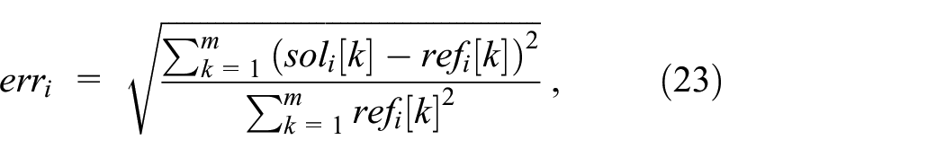
where
Names of different variations.
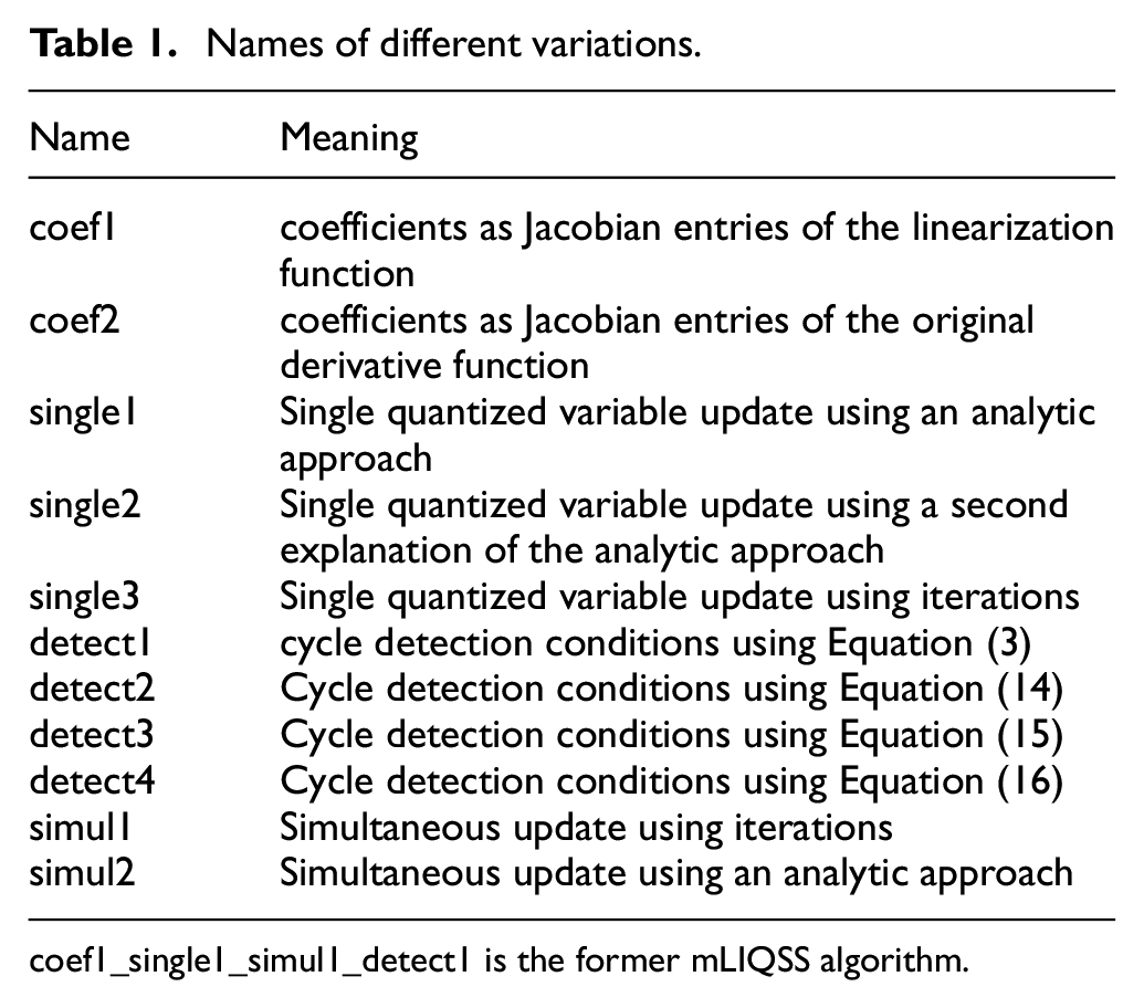
coef1_single1_simul1_detect1 is the former mLIQSS algorithm.
4.1. The Tyson model
The first problem is a model that is of great interest in the field of biology. The Tyson model describes the mechanism of a cell: the division, the growth, and the interactions among its components.
6
The model contains six components (
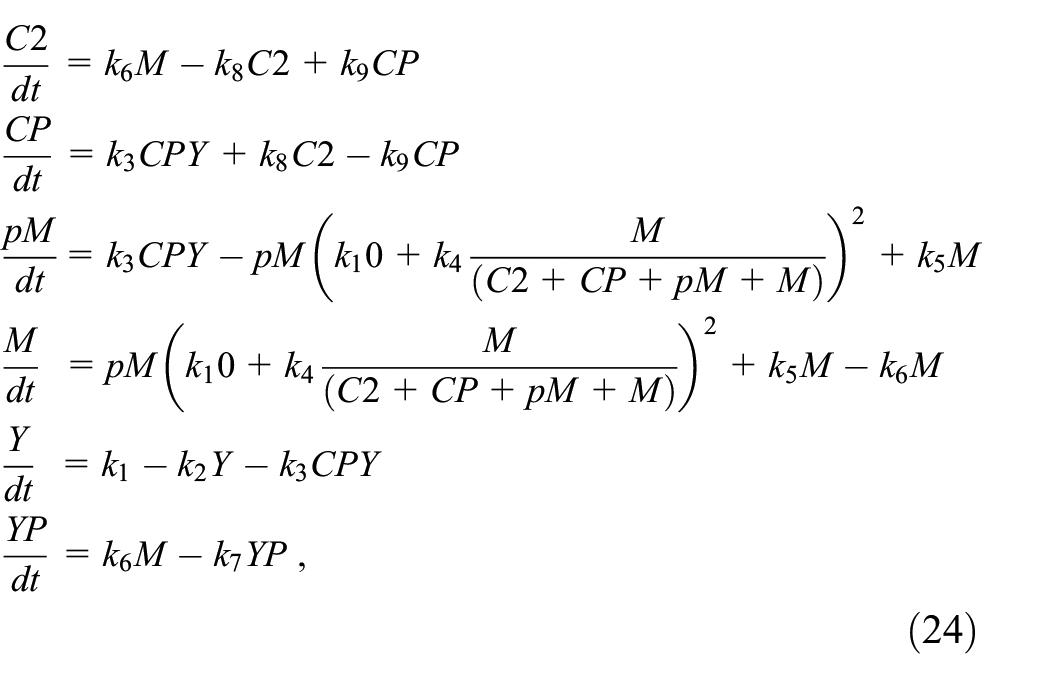
where
We simulated this system at tolerance values
4.1.1. Single and simultaneous updates
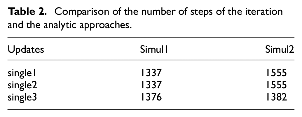
Table 2 compares the iteration and the analytic approach. The number of steps is slightly higher in the single update with iterations due to possible small distances between
Comparison of the number of steps of the iteration and the analytic approaches.
4.1.2. Cycle detection mechanism
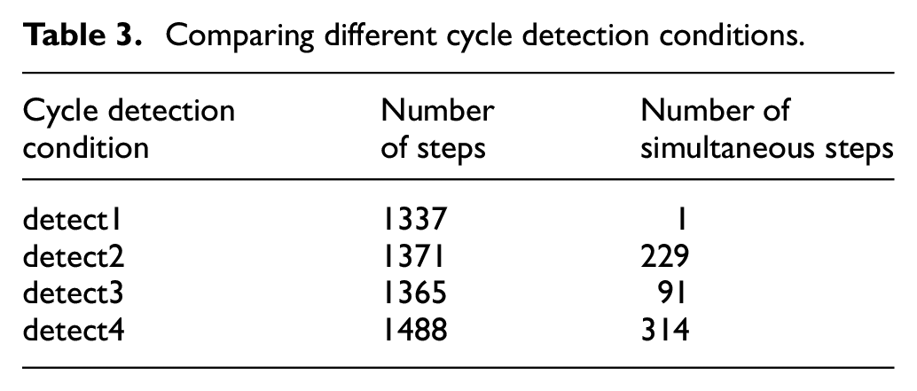
Table 3 shows that there is no improvement in any of the different cycle detection mechanisms while using the former method of updating the linear coefficients.
Comparing different cycle detection conditions.
4.1.3. Linear approximation coefficient
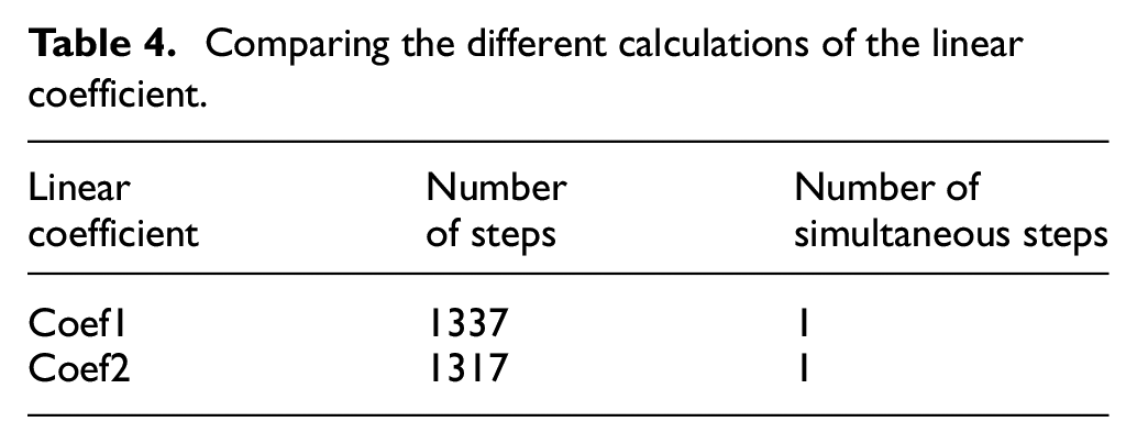
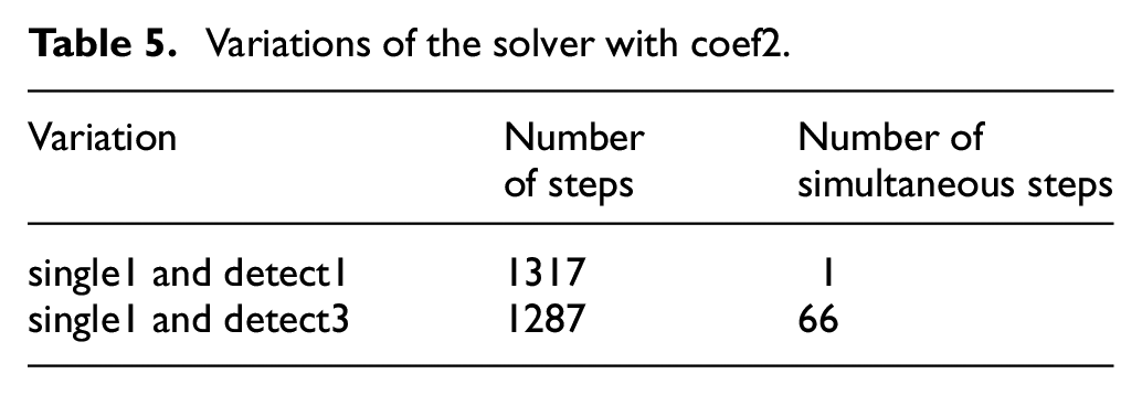
Table 4 shows that the use of the Jacobian of the original derivative function is slightly better than the former method of computing the linear coefficients because the two drawbacks of the former method do not occur frequently. In this case, a simultaneous update is performed only once. On the other hand, if the detection mechanism
Comparing the different calculations of the linear coefficient.
Variations of the solver with coef2.
4.1.4. Comparison of final version with former version and other solvers
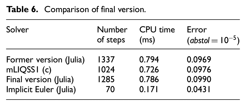
Table 6 shows the results of the final version (coef2_single1_simul1_detect3) of mLIQSS compared with the former version as well as other state-of-the-art solvers. The two modifications improved slightly the final mLIQSS (Julia), and with close results to the final version of mLIQSS1 (c). All mLIQSS solvers did not perform better than the Implicit Euler because the Tyson model is not a large sparse system.
Comparison of final version.
4.2. The Advection Diffusion Reaction problem
The Advection Diffusion Reaction equations describe many processes that include heat transfer, chemical reactions, and many phenomena in areas of environmental sciences. They are ODEs that result from the method of lines (MOL). The resulting system in Equation (26) is a large stiff system with possible large entries outside the main diagonal: 6
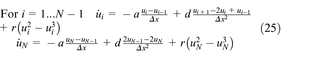
where N is the number of grid points and
Further explanations can be found in Bergero et al. 14
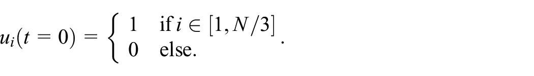
We simulated this system until a final time
4.2.1. Single and simultaneous updates
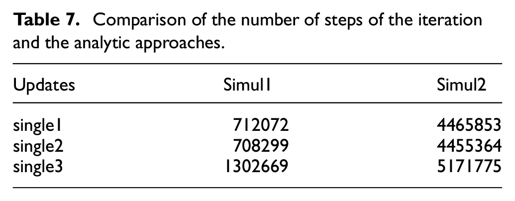
As seen in the Tyson model, Table 7 shows that the number of steps in the iteration approach is higher for the single updates and lower for the simultaneous update. The number of steps is not exactly the same for the two analytic approaches because they differ in the way they rely on the coefficient
Comparison of the number of steps of the iteration and the analytic approaches.
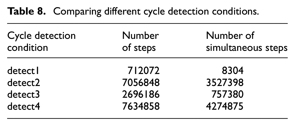
4.2.2. Cycle detection mechanism
Table 8 shows that there is no improvement in any of the different cycle detection mechanisms while using the former method of computing the linear coefficients.
Comparing different cycle detection conditions.
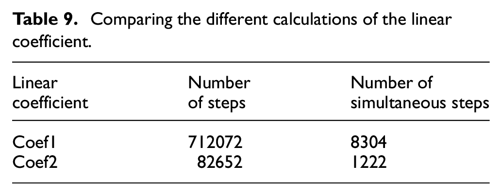
4.2.3. Linear approximation coefficient
Table 9 shows that the benefit of using the Jacobian of the original derivative function is more obvious in this problem as the number of variables and the number of simultaneous updates are higher. The final version is better because it uses more accurate coefficients while performing more simultaneous updates. In addition, the results of the two analytic approaches are the same because the linear coefficient is more accurate, and the cycle detection mechanism
Comparing the different calculations of the linear coefficient.
Variations of the solver with coef2.

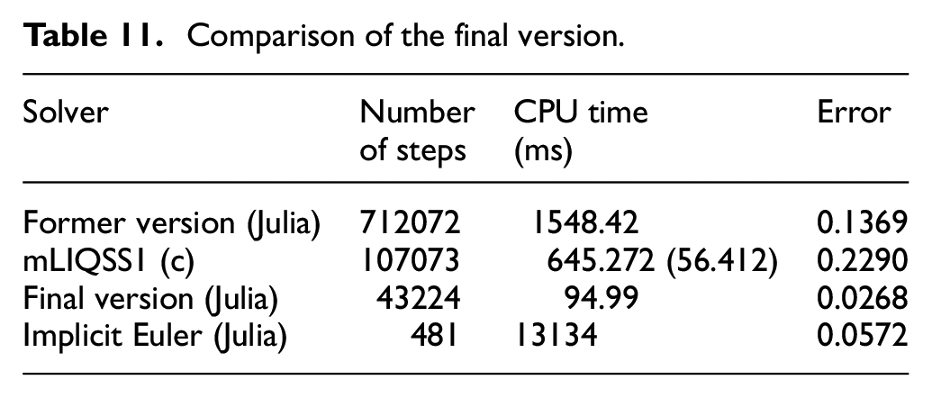
4.2.4. Comparison of final version with former version and other solvers
Table 11 shows the results of the final version of mLIQSS compared with the former version as well as other state-of-the-art solvers. First, this problem shows clearly the advantages of the two modifications in the final version of the solver. The final version of the solver is better than the former version and the mLIQSS1 (c) solver. Two different CPU times are recorded for this latter solver. The first time is the total run time including the initialization, simulation, and save times. The second is only the simulation time. In addition, all mLIQSS solvers are better than the Implicit Euler because the Advection Diffusion Reaction problem is a large sparse system.
Comparison of the final version.
5. Conclusion
Quantization-based methods demonstrated encouraging results, particularly in dealing with large sparse stiff models and scenarios characterized by frequent discontinuities. Despite considerable research that aimed to enhance their efficiency, there remains scope for further improvement, as quantization-based approaches continue to be an evolving area of study. In this work, we performed the following tasks. First, an investigation of current approaches to update the quantized variable is conducted. Then, two modifications are introduced and tested in the Tyson model and the Advection Diffusion Reaction system. The main findings are as follows:
An iteration approach in the single update of the quantized state performed worse than the existing analytic approach because the iteration approach can lead to small distances between the variable
An alternative explanation to the existing analytic approach, which can be more easily extended to higher orders, is presented and tested.
The analytic approach in the simultaneous update proved ineffective because maximizing the distance
Through an integration of the Jacobian entries of the original system, a more precise cycle detection and an adaptive step size are achieved.
Modifications of the cycle detection mechanism slightly improved performance.
With this investigation, QSS methods further solidify their position as powerful tools for simulating dynamic systems across various domains where traditional methods may struggle to maintain accuracy and efficiency. Regarding future work, we are considering the following:
Investigating the effect of the modifications on higher order solvers and in other stiff systems.
Conducting an error analysis considering these sources of error: the linear approximation, the quantization, and the cycle detection, in conjunction with the work presented in Mahawattege and Nutaro. 8
Footnotes
Funding
This research received no specific grant from any funding agency in the public, commercial, or not-for-profit sectors.