Frameworks for offshore wind farm installation scheduling with complementary application strategies using MILP and Petri nets

Abstract

The scheduling of offshore wind farm (OWF) installations is a complex, weather-driven, and resource-constrained problem. Mixed-integer linear programming (MILP) models excel at cost and makespan optimization, but remain difficult to verify and validate beyond feasibility checks. Similarly, Petri nets (PNs) provide behavioral transparency and simulation fidelity, yet lack prescriptive optimality. This article presents frameworks that utilize complementary application strategies to address two key needs, thereby combining the strengths of both approaches. First, an iterative verification–validation framework is employed that derives local PN models from MILP solutions and compares them with knowledge-based PN representations using conformance and reachability checks. Implemented in a simulation environment for the installation of OWF, the framework enables consistent model verification, cross-model validation, and context-aware scheduling. Second, a cascading decision-support framework that selects or blends MILP, heuristic, and PN-based scheduling methods through standardized descriptors and context signals. Numerical experiments demonstrate that optimization minimizes offshore time and cost, but requires high computational efforts. In contrast, Heuristics deliver short-term plans rapidly, while PN-based schedules offer intermediate costs and longer planning horizons, demonstrating that hybrid, context-sensitive orchestration outperforms any single method.

Keywords

offshore installations complementary model use mathematical optimization Petri nets heuristics verification and validation

1. Introduction

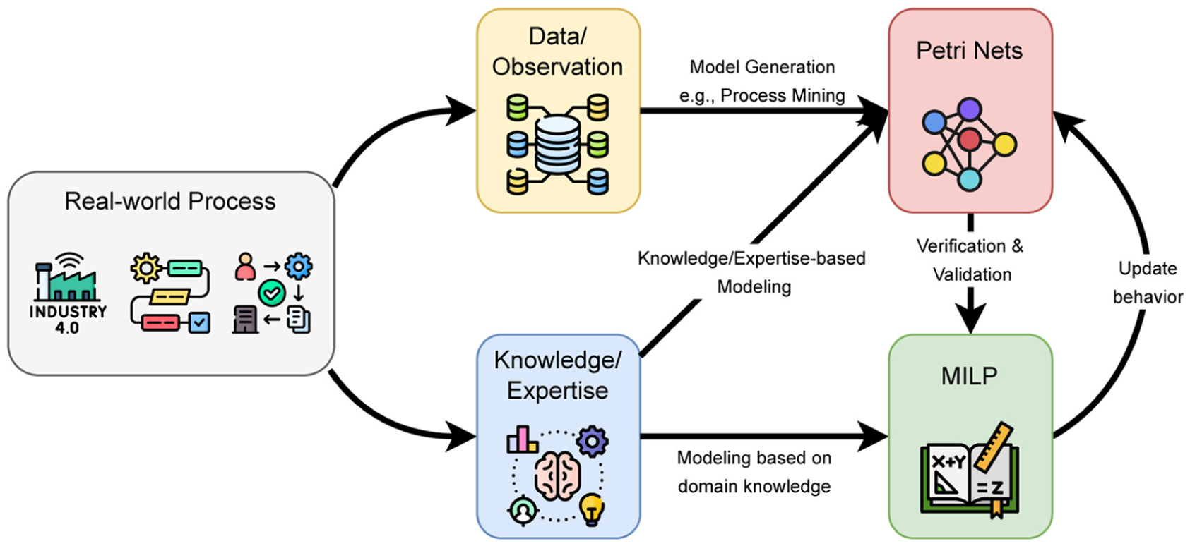
The installation of offshore wind farms (OWFs) is a highly cost-intensive logistic problem that couples cyclic vessel operations with narrow, safety-critical weather windows. Planning errors can quickly propagate into offshore time and charter costs, making prescriptive models attractive but also risky if they are not sufficiently validated. While heuristic approaches yield satisfying results, other modeling paradigms have gained prominence in the literature. The mixed-integer linear programming (MILP) approach is widely adopted for prescriptive scheduling because it encodes constraints precisely and can deliver provably optimal or bounded-suboptimal plans, especially when embedded in model-predictive schemes aligned with short-term forecasts. Petri nets (PNs) provide a mathematically grounded graphical formalism. They support process mining–based discovery and replay-style conformance checking, supporting the detection of deadlocks, unreachable states, and missing causal dependencies. These properties make PN a natural complement to MILP. In this work, we focus on the complementary application of these different approaches.

First, verifying that a large MILP model actually captures all admissible behaviors and validating it beyond feasibility and case-study outcomes remains difficult in practice. In addition, there are limitations to feasibility-only checks and model validation based on result comparisons. Typical verification focuses on consistency and feasibility, and validation often reduces to comparing schedules or KPIs between methods or scenarios. These steps do not ensure that feasible plans are operationally legal under domain logic, nor that the formulation admits only legal behaviors. Therefore, previous work motivates more formal behavior-level validation beyond simply matching numerical results.

Second, a structured decision-making approach is crucial for making effective decisions. MILP provides optimal solutions, but can be fragile if models are incomplete, costly for large-scale problems, and slow under tight deadlines. Alternatively, a PN-based method ensures transparency, provides formal guarantees on reachability, and allows for simulation-driven checks. However, it does not guarantee global optimality. Heuristics, on the contrary, create quick, satisfactory plans and are adaptable when predictions change or disruptions occur, although they sacrifice guarantees and might deviate from fundamental logic if not carefully managed.

In this work, we propose frameworks that use complementary application strategies to address these issues, that is, to leverage the strengths of each while mitigating the weaknesses of the others.

First, we build on an iterative verification and validation framework that transforms MILP schedules into PN models and tests them against a knowledge-based PN of the domain. Each iterative solution logs the first feasible solution, all improved solutions, and the final incumbent. Afterward, the strategy derives compact local PNs from these event logs, capturing the causal and resource allocation relations within each possible solution. We then conduct the following: (1) Verification via language inclusion and token replay/alignments to assess robust timings. (2) Structural analysis (reachability, liveness, boundedness) to expose latent deadlocks, unreachable tasks, or resource conflicts that feasibility checks can miss. Counterexample traces are translated into targeted MILP refinements (e.g. missing precedence arcs, minimum-stay constraints, weather buffers), after which the problem is re-solved and re-logged. The loop ends when inclusion holds, replay fitness exceeds a threshold, and no safety or capacity-violating markings are reachable. Final PN simulations under sampled weather provide confidence intervals for key performance indicator(s) (KPIs), yielding schedules that are both cost-efficient and behaviorally admissible.

Second, in the complementary decision-support framework, a decision-management module governs method selection and blending through standardized model descriptors (capabilities, compute footprints, robust profile) and context signals (forecast reliability, time-to-decision, cost priorities, risk tolerance). At each planning epoch, the module evaluates candidate schedulers, MILP, PN-based, and heuristic, and applies a policy that can (1) select a single method, (2) blend outputs (e.g. use a heuristic for rapid recovery and MILP for overnight refinement), or (3) cascade methods (heuristic → MILP warm start → PN sanity check). Outputs are normalized into a unified schedule representation and guarded by safety and compatibility checks. Fallback rules ensure time-critical dispatch when compute budgets or forecast horizons are tight, while a stability regularizer limits gratuitous changes to already-committed actions.

The contributions of this work can be summarized as follows.

A complementary MILP-PN framework for OWF installation that unifies prescriptive optimization with behavioral verification and validation via language inclusion and replay-fitness checks against a knowledge-based PN.

Receding-horizon prescription with incumbent logging, aligned to weather forecasts, and producing rich event logs and structural traces for PN discovery, improving behavioral coverage without excessive computation.

A decision-support architecture and strategy that standardizes model descriptors and outputs, enabling context-aware selection and hybrid use of optimization, heuristic, and PN-based schedulers; results clarify cost/compute/stability trade-offs for practical planning under uncertainty.

This article builds on previous work presented at several conferences, including SIMS’25¹ and ANNSIM’25,² where initial versions of the verification and validation framework were discussed. In this work, these ideas are consolidated and integrated to illustrate various application scenarios in which the complementary use of multiple modeling paradigms improves both theoretical and practical outcomes.

In addition to unifying previous contributions, this article introduces a decision-support framework and includes several simulation studies. The results of these studies demonstrate the managerial and operational advantages of having access to and, in particular, combining different scheduling methods. In general, the study shows that complementary strategies not only strengthen theoretical developments, particularly in verification and validation, but also improve practical decision-making performance.

2. Literature review

The scheduling of OWF installations is particularly challenging due to the volatility of environmental conditions and operational interdependencies. Prescriptive MILP models are often employed to optimize cost-related objectives under such uncertainty.³ However, their validation is nontrivial because true ex post validation would require the adoption and repeated execution of the optimized policy by decision-makers.⁴ PNs provide a complementary formalism for modeling and analyzing the behavior of installations.⁵ Due to their rigorous mathematical foundation and intuitive graphical notation, PNs facilitate transparent modeling and are frequently validated by conformance checking (replay) against observed or simulated behavior.⁶

A comparative study in Peng et al.⁷ indicates that MILP- and PN-based approaches can yield comparable schedules under matched scenarios (e.g. identical start date and offshore dynamics). Rippel et al.⁸ propose a model-transformation interface to ensure scenario parity across the different modeling paradigms. Nevertheless, post hoc comparisons of schedules do not constitute a formal cross-model validation method, motivating an iterative verification and validation scheme that integrates both formulations.

2.1. Iterative verification and validation

Linear and MILP models are widely applied, from clinic scheduling⁹ to machine learning optimization.¹⁰ Here, we focus on MILP as a prescriptive tool for scheduling and on the corresponding verification and validation practices.

2.1.1. Verification

Several verification techniques are well-established for developing MILP models. The core procedures include checks for logical consistency¹¹ and feasibility analysis¹² to ensure technical correctness. In practice, modelers (1) verify the mathematical formulation, confirming logical implications, constraint correctness, and whether the objective function encodes the intended goal; (2) perform unit tests of constraints in isolation to confirm that they restrict the feasible region as intended; (3) confirm bounds and domains (e.g. non-negativity, capacities) are properly defined; and (4) run the model on simplified or known data to ensure that the solver returns feasible solutions satisfying all constraints. Modern solvers such as CPLEX¹³ and Gurobi¹⁴ further support debugging through detailed logs (numerical warnings, infeasibility diagnostics). Sensitivity analysis is commonly used to assess the effects of parameter perturbations and to test whether the model behaves as expected under input changes.¹⁵

2.1.2. Validation

Validation concerns suitability for the intended use. McCarl and Apland⁴ distinguish predictive and prescriptive models and argue that the ultimate validation of a prescriptive model is its adoption in practice. Consequently, validation procedures for prescriptive MILP models are often informal, including (1) face validation, (2) scenario analysis, and (3) stress testing; expert and stakeholder reviews are common.¹⁶ Many studies emphasize numerical case studies without dedicated validation protocols; for instance, Pinzon et al.¹⁷ present an MILP with 48 constraints and performance results, but no formal validation step. Other contributions improve trustworthiness by enabling independently verifiable certificates for MILP solutions.¹⁸ Case-specific validations also appear: Kunath et al.¹⁹ conduct historical-data scenario analysis in a chemical batch setting, while Han et al.²⁰ evaluate two flexible job-shop MILP formulations on 10 hypothetical instances. Overall, systematic and effective validation methods for prescriptive MILP models remain limited.

2.2. Offshore scheduling and model selection

Research on offshore wind installation planning spans optimization models, simulation frameworks, and heuristic strategies addressing weather uncertainty and logistics. Although these contributions have advanced the field, they are typically presented in isolation, which hampers systematic comparison and impedes context-sensitive selection. This subsection reviews planning methods and their challenges, outlines model-comparison approaches, and identifies the gap motivating the framework proposed here.

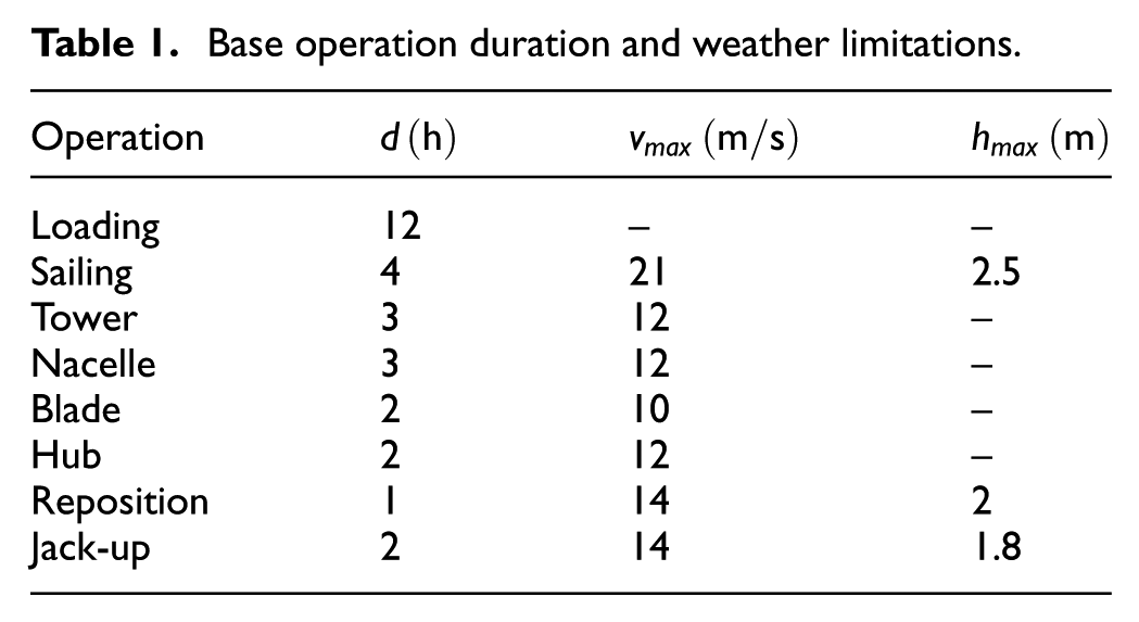
Offshore wind turbine (OWT) installation is a structured yet weather-sensitive process.³ A jack-up (JU) vessel positions at a site, jacks up, and assembles turbine components sequentially before relocating. Tasks such as loading, lifting, and jacking are constrained by environmental thresholds, especially wind speed and wave height. Exceeding these thresholds during operations causes delays or aborts, resulting in lost progress and costly idle time. Weather windows are more frequent from April to October, concentrating offshore work within this period. Consequently, scheduling efficiency is critical for cost control and motivates decision-support models.

Despite extensive offshore wind research, relatively few studies address detailed installation planning.²¹ Existing work analyzes weather modeling,²² installation concepts,^21,23 fleet composition,²⁴ and broader decision support,²⁵ alongside vessel scheduling and cost optimization.^26,27 Port-side constraints are less studied. Notable exceptions include Beinke et al.²⁸ on shared vessels and port bottlenecks and Oelker et al.²⁹ on storage requirements. Most contributions instead develop models to optimize or simulate offshore operations under specific assumptions and data regimes.

Representative approaches include the following:

Heuristic solutions with generated weather data:³⁰ mathematical modeling with heuristic techniques and synthetic weather using probabilistic transition matrices and Weibull distributions.

Stochastic integer programming:²⁷ historical weather data with Benders decomposition to solve a stochastic installation scheduling problem.

Variable Neighborhood Search:²⁶ heuristic optimization based on averaged historical weather data for decommissioning scenarios analogous to installation.

Receding-horizon planning:³¹ short-term forecasts and real-time data embedded in a mixed-integer linear program within a rolling-horizon framework.

Simulation-based optimization:³² cascading simulation to evaluate discrete installation strategies, combining forecasts with long-term weather records.

Timed Petri nets:⁷ token-based state transitions derived from historical weather data to model installation processes.

Each approach introduces distinct strengths and limitations. Some excel at detailed operational constraints; others prioritize computational speed or robustness under uncertainty. These approaches are not mutually exclusive; instead, their differences invite complementary use, tailoring selection or combination to evolving project requirements, data availability, and planning horizons. Nevertheless, most studies present models in isolation, leaving practitioners without structured guidance for joint application or principled selection.

The systematic comparison of planning models remains challenging across domains.³³ Individual evaluations often emphasize performance metrics (runtime, solution quality) while overlooking methodological and structural differences that determine the applicability of a solution to specific contexts. This limitation is widely acknowledged³⁴ and is particularly pronounced in offshore installation planning, where models differ in scope, assumptions, and data requirements. Other fields have developed structured comparison methods, such as theoretical classifications,³⁵ standardized test cases,³⁶ and harmonized empirical evaluations.³⁷ For example, Gils et al.³⁶ show that the abstraction level strongly influences the results of energy system modeling. In contrast, Schweiger et al.³⁸ employ expert-based comparisons for cyber-physical systems. These studies provide valuable but largely static insights tailored to fixed models or use cases, and they seldom support real-time, cross-context decision-making where planners must choose among heterogeneous tools. What is missing is a flexible decision-support concept that enables models to be described, compared, and combined dynamically, using standardized model descriptions, interoperable architectures, and decision-support tools to guide selection in a structured, context-sensitive manner.

2.3. Research gaps and contributions

In this subsection, we discuss the research gaps and emphasize our contributions based on the literature review conducted.

2.3.1. Iterative verification and validation

Prescriptive MILP models are often evaluated through case studies, whereas predictive models can be validated using historical data. However, historical data are insufficient to rigorously validate prescriptive models. Several factors explain the gap: Translating a real-world decision problem into a tractable MILP demands expert choices, including simplifying assumptions, linearizations, and logical encoding, which are complex, error-prone, and partly subjective. Local checks of constraints and feasibility do not guarantee that the global formulation captures system reality. Feasibility certifies compliance with the mathematical model, not operational acceptability in practice, so feasible solutions can still be inconsistent with actual behavior. Prescriptive models yield detailed schedules judged by user-defined criteria, such as makespan. However, a meaningful empirical comparison would require observations generated under the very optimal policy being proposed, data that typically do not exist. McCarl and Apland⁴ argue that true validation comes from the adoption of decision-makers through implementation and repeated measurement, creating a paradox: managers hesitate to adopt an unvalidated model, even though adoption is the basis of validation.

To address these challenges, we propose an iterative verification and validation framework that couples prescriptive MILP with a simulation-based digital twin. Batty³⁹ instantiated in PNs, a formalism well suited to model concurrency, synchronization, and resource allocation, with a rich analytical toolbox for dynamic behavior.^40,41 The PN layer emphasizes system behavior and, when combined with simulation-based optimization, supports established practices in scheduling and control.⁴² Moreover, contemporary process mining techniques enable the construction of PNs that are faithful to observed operations.⁴³ Our contributions on verification and validation are twofold.

Verification: We derive a PN from MILP solutions to provide a systematic, state-space view that can reveal issues (e.g. deadlocks) that elude purely algebraic checks.

Validation: We build a PN from real-world observations (through process discovery) and replay MILP-induced schedules within the twin, allowing safe, repeated ex post experiments; statistical measures (e.g. confidence levels) then quantify the degree of validation without incurring real operational risk.^39–43

2.3.2. Complementary decision support

The growing variety of planning models in offshore wind installation, spanning optimization, simulation, and heuristic approaches, reflects the domain’s complexity and the maturity of specialized research. However, this diversity has not been matched by integrative frameworks that clarify how different models relate to each other, how they can be selected for specific contexts, or how they might be used in combination. As a result, model choice in practice remains ad hoc, often driven by familiarity or disciplinary convention rather than operational suitability, which limits the ability to leverage each paradigm’s strengths across various project stages, data regimes, and decision-support needs.

This article addresses this gap through a structured framework that supports the systematic understanding and complementary use of various planning models. Unlike prior comparison studies, which are often narrowly scoped or static, the proposed framework provides interoperable interfaces, standardized descriptors, and a decision-support architecture that enables models to be compared, selected, and combined dynamically. In doing so, it advances the state of the art by shifting the focus from identifying a single “best” model to enabling hybrid, context-sensitive approaches that better reflect the complexity of real-world offshore wind projects.

3. Preliminaries

3.1. OWF installation process

The installation of OWFs can be viewed as a process comprising numerous installation cycles (ICs), during which the installation vessel navigates between the base port and the construction site, executing sequential offshore operations. Fundamentally, an IC can be divided into five different operation categories: (1) installation, (2) sailing, (3) reposition, (4) JU and jack-down (JD), and (5) loading. 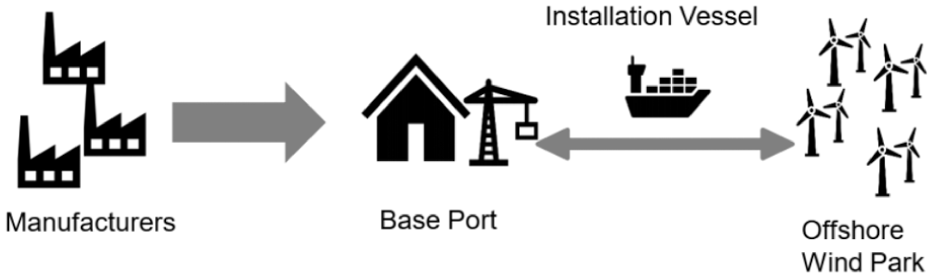Operations, except for (2), occur in an IC at least once and at most $N_{C, \max}$ times, where $N_{C, \max}$ is the maximum capacity of the installation vessel. In addition, each operation has a base operation duration and is limited by varying offshore weather conditions. The duration of the base operation and the weather limitations of each operation are summarized in Table 1. In the table, d denotes an operations base duration if it is not interrupted by bad weather, $v_{\max}$ denotes the max wind speed (velocity) and $h_{\max}$ denotes the maximum wave height for the operation. Furthermore, in this work, the conventional logistic concept is considered, as described in detail by Rippel et al.³¹ The installation of OWF wian OWF using the conventional logistics concept is depicted in Figure 1.

Figure 1.

Conventional concept: OWF installation process.

Table 1.

Base operation duration and weather limitations.

Operation	$d (h)$	$v_{\max} (m / s)$	$h_{\max} (m)$
Loading	12	–	–
Sailing	4	21	2.5
Tower	3	12	–
Nacelle	3	12	–
Blade	2	10	–
Hub	2	12	–
Reposition	1	14	2
Jack-up	2	14	1.8

3.2. MILP model

This article uses results generated using the MILP model presented by Rippel et al.³¹ and shown in Appendix 1. The model consists of 20 distinct constraints, each instantiated over the selected prediction horizon and the number of vessels. At default settings, covering one vessel and a 2-week prediction horizon, the generated problems regularly involve more than 4000 integer and binary variables, as well as constraint matrices with more than 5000 rows, 4000 columns, and more than 86,800 non-zero entries.

The model provides an optimal schedule for offshore operations while considering the uncertainty of weather forecasts through discretization via stochastic simulations.³¹ The objective function of the model aims to minimize the costs incurred by operations, particularly during offshore times, while maximizing the number of turbines installed within a given time interval. The authors embed MILP optimization within a model-predictive control scheme to counteract the increasing uncertainty of weather forecasts by applying predictive online optimization. This receding-horizon scheme iteratively solves several instances of the MILP model with smaller planning horizons (typically around 2 weeks) to minimize the impact of forecasting uncertainties and keep the scheduling problem’s dimensions manageable.

Consequently, the optimization model is embedded within a larger simulation model that simulates weather conditions and the progress of an installation project, incrementally obtaining smaller optimal plans. For this article, the solver was instructed to record all viable solutions, optimal or not, to ensure a large coverage of possible behavior with a limited number of simulation runs.

3.3. Petri nets

As discussed in Section 1, PNs are used for two major purposes: (1) as a general approach to model the OWF installation process and (2) as the output of process mining algorithms, that is, the process model. To address research gaps, we introduce the following PN formalisms.

Definition 1. Petri net.⁴¹A (conventional) PN is a 5-tuple:

P N = (P, T, F, w, M_{0})

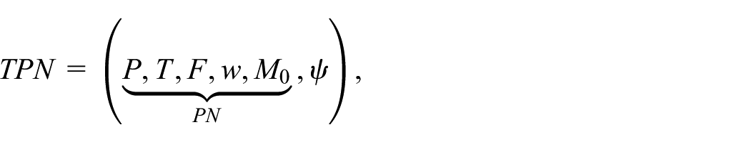
where P is a finite set of places, T is a finite set of transitions, $F \subseteq (P \times T) \cup (T \times P)$ is the set of flows, $w : F \to Z^{+}$ is weight function that maps arcs to a positive integer-valued weight, and $M_{0}$ is the initial marking. The intersection of the set of places and the set of transitions is the empty set, that is, $P \cap T = \emptyset$ . A PN without marking is referred to as a PN structure, consisting of the first four elements of PN, denoted by N = (P, T, F, w). Thus, a PN can be written as PN = (N, M₀).

PNs are called safe when each place can hold at most one token. PNs are called pure if there is no self-loop in the net.

Definition 2. Timed Petri net.⁴⁴Timed Petri nets (TPNs) are mathematically defined as a 6-tuple:

T P N = (\underset{P N}{\underset{︸}{P, T, F, w, M_{0}}}, ψ),

where the tuple $(P, T, F, w, M_{0})$ forms a (conventional) PN introduced in Definition 1. The notion of time is introduced by the mapping $ψ : T \to P^{+}$ , which is a firing time function that assigns a positive real number to each transition on the net. Wang⁴⁴and Popova-Zeugmann⁴⁵are referred for more details and information on TPN.

Unlike the MILP approach, PNs are naturally associated with graphical representations, which are shown in Figure 2. In this work, we distinguish between invisible, immediate, timed, and discrete-time Markov chain (DTMC)-timed transitions. Fundamentally, an invisible transition (represented by a solid square) is an immediate transition without a name/label, which is used to model invisible mechanisms in the process or simply used to satisfy the constraints associated with PNs. The DTMC transitions are special timed transitions. They obtain the estimated firing time from the DTMC predictor introduced in the work by Rippel et al.,³¹ which utilizes historical weather data from the German North Sea from 1958 to 2007.

Figure 2.

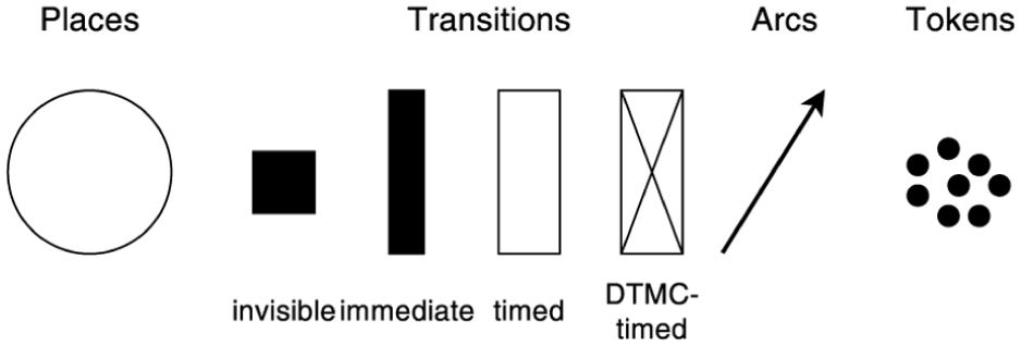
Graphical elements of PN models.

As mentioned in Definition 1, the state of the PN is given by the markings. A marking M indicates the current token distribution, that is, the number of tokens stored in each location. A marking can be written as a vector, where the i th component stands for the number of tokens of i th place. The dynamics of the PNs are controlled by the firing of the transitions, which remove/add tokens from/to their input/output places. An example is given in Figure 3, where the PN is transitioned from state $M_{1} = [10, 0, 0, 0]$ to state $M_{2} = [8, 1, 1, 0]$ . A transition t is considered enabled, that is, ready for firing, when the number of tokens in all the input places of the transition t, denoted by $• t = {p | (p, t) \in F}$ , is greater than or equal to the weight of the associated arc. The set of output places is denoted by $t • = {p | (t, p) \in F}$ accordingly. Taking the transition $t_{1}$ of the PN depicted in Figure 3 as an example, the set of input places of $t_{1}$ is $• t_{1} = {p_{1}}$ and the set of output places is $t_{1} • = {p_{2}, p_{3}}$ . In Figure 3(a), place $p_{1}$ contains 10 tokens, which is larger than the weight of the associated arc $w (p_{1}, t_{1}) = 2$ . Thus, the transition $t_{1}$ is enabled. The firing of transition $t_{1}$ removes two tokens from $p_{1}$ and adds one token to both $p_{2}$ and $p_{3}$ . Figure 3(b) depicts the state of the PN after the firing of $t_{1}$ , that is, $M_{2} = [8, 1, 1, 0]$ .

Figure 3.

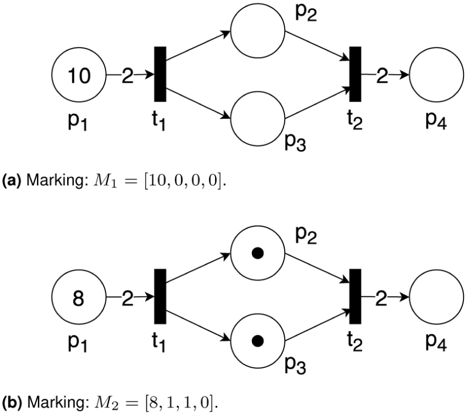
Example: conventional Petri nets. (a) Marking: $M_{1} = [10, 0, 0, 0]$ . (b) Marking: $M_{2} = [8, 1, 1, 0]$ .

In the literature, several PN-based models have been proposed to handle the scheduling problem in the offshore installation domain.⁴⁶ In this work, we follow the TPN model for offshore installation introduced in the work by Peng et al.⁴⁷ The formal definition and dynamics of the TPN models are presented in Murata,⁴¹ which is based on the fundamental principles of PN dynamics. When a timed transition fires, the associated clock of the TPN increments with the corresponding transition firing time. Figure 13(a) shows the TPN model used in this article.

In this work, we unfold the proposed cyclic TPN and embed all possible operations explicitly considering a vessel capacity of four; that is, an installation vessel can load a maximum of 4 offshore wind turbines. To simplify the later validation procedure, we combine several operations introduced in the last subsection together and enumerate them as follows: OP1—installation, OP2—sailing back to port (back), OP3—sailing to the construction site (forth), and OP4—loading. Furthermore, we add the number of occurrences to the notation. For example, OP1-3 means that operation 1 has been performed 3 times.

3.4. Process mining

Process mining is an interdisciplinary field focused on constructing detailed process models from event logs to facilitate in-depth analysis. As modern information systems generate large volumes of data, efficiently building process models from these data sets is a challenge. Various discovery algorithms have been developed to address this problem, creating diverse models such as transition systems (TS), PNs, and Business Process Modeling Notation.⁴³ Our study concentrates on PNs due to their robust mathematical framework and their effectiveness in representing complex processes.

Definition 3. Language and Overapproximation.⁴⁸The language of a system, denoted by $L (S)$ , is the set of all possible sequences feasible from the initial state. For two systems S₁ and S₂, S₂ is called an overapproximation of S₁, when $L (S_{1}) \subseteq (S_{2})$ .

Definition 4. Trace and Event Log.⁴³Given the universe of activities $A$ , a trace $σ = < a_{1}, \dots, a_{n} > \in A^{*}$ is a sequence of activities, where $A^{*}$ is the Kleene closure of the set $A$ . An event log is a multiset of traces, that is, $L \in B (A^{*})$ .

Definition 5. Process Mining Problem.⁴⁹The objectives of the process mining problem can be articulated as follows: given an event log L from system S, we are searching for a preferably small finite marked PN, s.t. 1) $L (S) \subset L (P N)$ ; and 2) $L (P N) \ L (S)$ is minimal, which implies that the learned PN should be the tightest overapproximation over S.

3.5. Evaluation criteria

In this work, we need two metrics: (1) to measure the relations between two models and (2) to qualify the model validation results.

The language of a PN, $L (PN)$ , is the set of all possible firing sequences. Two models are bi-similar if they share the same language. Model $M^{'}$ is included in model M, if $L (M^{'}) \subseteq L (M)$ .

The fitness measures how well a process model can reproduce the behavior observed in an event log. A model with perfect fitness can replay all recorded traces without deviations. In this work, the fitness measure based on token replay is used.⁵⁰

4. Iterative verification and validation framework

As mentioned in Section 1, complementary application strategies are fundamental to the iterative framework that verifies and validates MILP models using PN models. The holistic view is given in Figure 4. In particular, it uses the results generated by the MILP model to learn the PNs that represent these results. By comparison with the knowledge-based PN, modelers can cross-validate if the MILP’s generated solutions are completely covered by the PN, and vice versa. This feedback can be used as information for verification or validation based on model behaviors. The process follows the following steps:

Define and solve the MILP model and constraints, assuming that the real-world system is specified and the modelers have the necessary expertise in mathematical optimization and domain knowledge. Using standard procedures (see Section 2), we verify the MILP model to ensure logical consistency and mathematical feasibility.

Derivation of Petri nets. In this framework, we classify the PN models into three different types based on how they are generated:

2a. Knowledge-based PNs: Similar to constructing the MILP models, PNs can be built purely on the basis of domain knowledge. This can be accomplished through bottom-up procedures, for example, as described in the work by Zhou and Jeng,⁴² or by mining the model using generative AI.⁵¹

2b. Data-based PNs: Using process mining techniques,^43,52 PN models that conform to system behaviors can be derived from real-world observations, that is, event logs.

2c. Local PNs: Local PN models can be derived from the solutions generated by the MILP models. They are local because the solutions of MILP models are optimal schedules, that is, they do not contain all the behaviors of the system.

The inner verification loop. The inner verification loop uses local PNs generated from feasible solutions of the MILP model. Note that this verification step builds upon standard procedures such as the logical consistency checking done in Step 1. This loop includes the following sub-steps:

3a. Map the MILP solution to a PN model.

3b. Construct the reachability graph.

3c. Verify system constraints with PN analysis.

3d. Update and refine the MILP model.

Standard verification ensures logical consistency and feasibility, but solutions may still contain errors, for example, neglected constraints. This inner loop maps MILP solutions to PNs and employs reachability analysis to create a state-space representation. Analysts can observe potential pathways and transitions, which is useful in complex MILP models with constraints and resource dependencies. PN analysis detects issues like deadlocks,^53–55bottlenecks,⁵⁶ and resource conflicts.⁵⁷ Based on PN analysis results, modelers can refine and improve the MILP models. A numerical example of detecting and resolving deadlocks in the MILP model is presented in Subsubsection 6.1.1.

4. The outer validation loop. Similarly to the last step, the outer validation loop consists of the following main steps:

4a. derive a proper PN representation for the intended;

4b. construct the reachability graph;

4c. validate the model against expected outcomes; and

4d. update and refine the MILP model.

Notice that there are multiple ways to learn/create a PN model. In this study, we adopt a PN representation based on the criterion $L (M) \subseteq RG (PN)$ , which means that the language of the system must be complemented by that of the PN. This requires exhaustive observations of the system,⁵⁰ which are often lacking due to measurement errors, limited behavioral coverage, or short observation periods. Consequently, we distinguish between two approaches to the derivation of PN: (1) data-driven PN from observations and (2) knowledge-based PN from expert knowledge. While data-driven PNs generally offer more objective validation, they become unreliable when data are incomplete. In such cases, knowledge-based PNs serve as an effective alternative to system validation.

Figure 4.

Holistic view of the iterative framework.

Figure 5 illustrates the primary steps of the iterative framework, assuming we have access to both the knowledge-based PN model and the MILP model that require cross-validation. The framework covers three major stages. First, by defining a series of scenarios, modelers attempt to capture as much of the observable system’s behavior as possible. After defining these scenarios, the modelers use the MILP model to generate as many feasible solutions as possible. The framework recommends recording all incumbents generated during an optimization, as each incumbent represents a viable solution, even if it is not optimal. The second stage involves analyzing these solutions or the corresponding event logs to identify smaller data-driven PNs. Each of these nets covers all the states and transitions necessary to generate the same solution. Finally, the third stage covers the actual cross-validation. During this stage, modelers compare the languages spanned by the data-driven PNs with the language defined by the knowledge-based PN. In the best case, the set covers all the knowledge-based language and does not include additional constructs. If parts of the knowledge-based language are missing in the set, modelers might need to specify additional scenarios. In contrast, if the set of data-driven languages contains constructs not included in the validated knowledge-based language, it can be assumed that the MILP model allows for illegal solutions.

Figure 5.

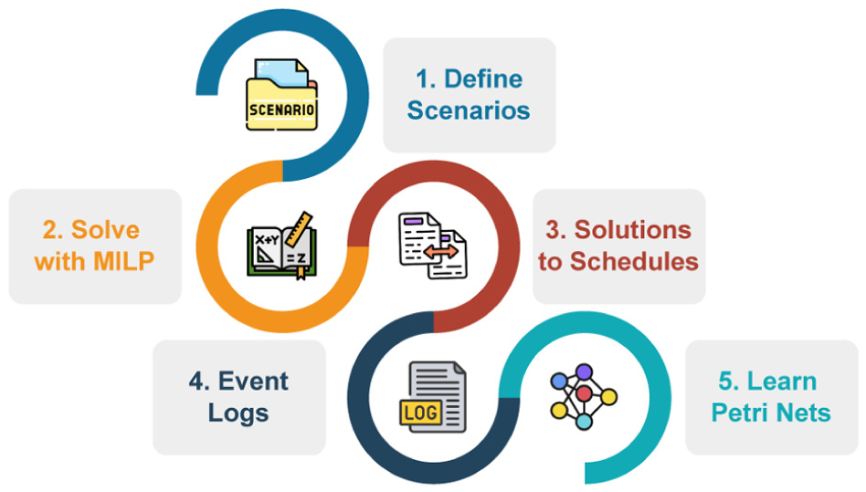
Workflow: major steps of learning Petri nets from MILP solutions.

While the comparison of the MILP-derived PN against the knowledge-based PN is termed “validation” in this framework, it is important to note that from a formal modeling and simulation (M&S) perspective, this can also be viewed as inter-model verification or model alignment.^58,59 As discussed in Section 2.3.1, the lack of sufficient historical data for prescriptive models necessitates the use of a reference model. This approach is consistent with established V&V techniques such as “Comparison to Other Models.”⁵⁹ Consequently, the validity of the MILP solution in this context is contingent upon the correctness and fidelity of the expert-designed PN. To mitigate risks of expert error, the knowledge-based PN in this study underwent iterative internal reviews by domain experts to ensure a high level of confidence in its representation of the offshore installation process.

5. Complementary decision-support framework

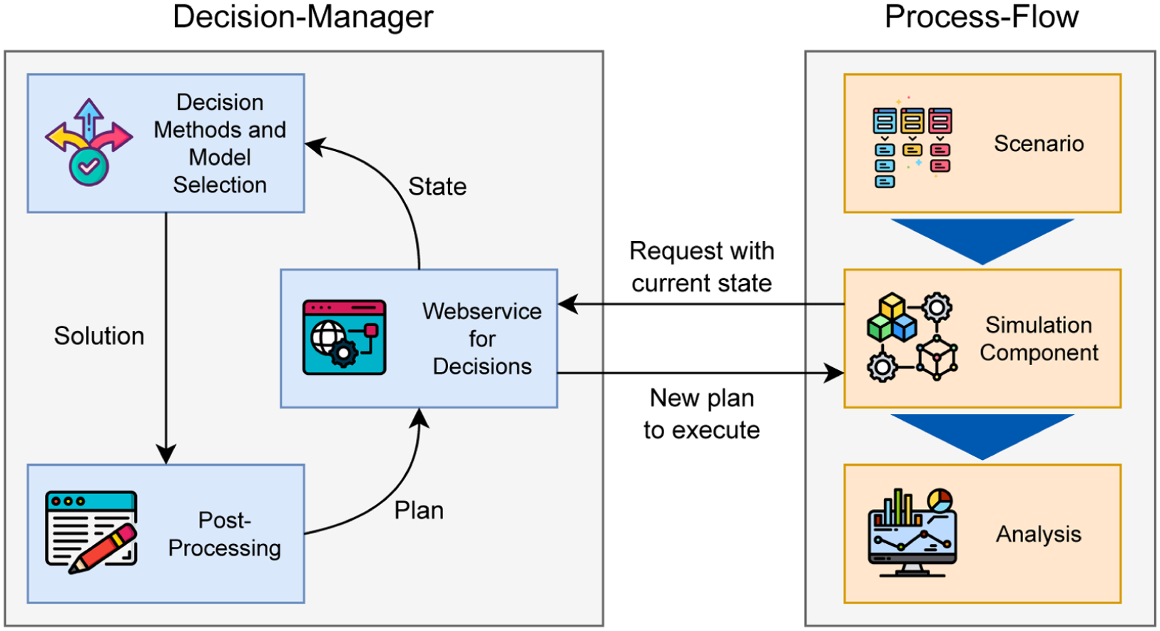
Similar to the verification–validation framework, this application strategy operationalizes model complementarity through a modular decision-support framework. This framework couples a process-flow simulation, which represents the OWF installation process and triggers context-dependent scheduling requests, with a central decision manager responsible for selecting, executing, and postprocessing decision methods, that is, scheduling methods (Figure 6).

Figure 6.

Component of the complementary decision-support framework.

At runtime, the simulation continuously evaluates system conditions, including weather forecasts, vessel availability, and project status. Whenever a so-called decision point is reached (e.g. a vessel requires a new work plan), it sends a structured request (JSON payload) describing the current state of the system. The decision manager analyzes the request, identifies the most appropriate (scheduling) method, and invokes it. This separation of process execution and method selection ensures transparency and facilitates the integration of heterogeneous models.

5.1. Framework: process-flow module

Scenario Definition: Both the simulation component and the decision manager rely on a structured description of an installation scenario (scenario), including information such as the number of turbines to be installed, their locations, the available vessels and their capacities, and other logistical constraints. To ensure consistency and transparency, the framework is based on a formal domain model that defines the relevant entities, their attributes, and the relationships between them. Such models are commonly expressed in Unified Modeling Language (UML) class diagrams or similar notations. This work applies an extended version of the domain model and modeling tool proposed by Rippel et al.⁸ and shown in Figure 20 in Appendix 3. While the domain model specifies the conceptual structure, the practical exchange of scenario data is realized through JSON formatted strings, which can be retrieved online by sending a get request (https://l3s-offshore-plan-2.l3s.uni-hannover.de/l3s-offshore-2/dto/example/scenario). Listing 1 shows some lines of the scenario object.

Listing 1: Excerpt of the scenario JSON.

{
…
"scenario_OWTsToBuild": 50,
"operation_name": [ "Install Tower", …],
"operation_duration": [ 3, 3, 2, 2, 2, 2, 4, …],
"operation_wind": [ 12, 12, 10, 10, 10, 12, 21, …],
…
"state_OWTsFinished": 0,
"state_currentDate": "15-Jun-2000",
"state_vessel_location": [ 0],
"state_vessel_availabeFromDate": [ "15-Jun-2000"],
…
}

Simulation: The simulation model constitutes the core of the process-flow module. Its task is to accurately represent the real-world installation process, capturing its typical progression and potential disruptions from external factors. In the context of offshore installation, weather is the dominant factor. The simulation, therefore, updates environmental conditions every hour, using historical weather records as input. Since each operation is restricted by wind speed and wave height thresholds (i.e. operation_wind and operation_wave in scenario), the model checks these values against the requirements of the currently active task. If conditions exceed the limits, the simulation aborts the operation and restarts it once a suitable weather window reappears. This mechanism enables the simulation to accurately reproduce realistic waiting times and interruptions, which have a significant impact on project schedules and costs.

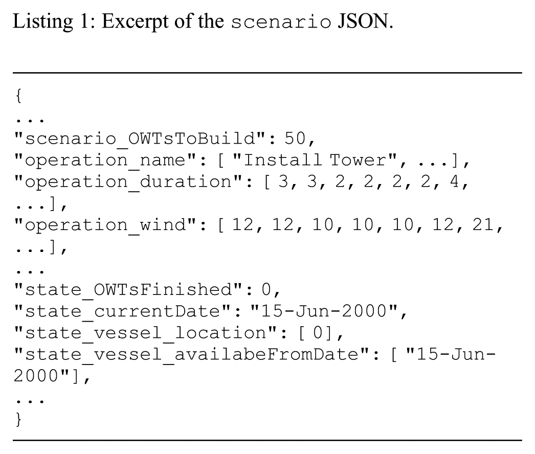
For the work presented in this article, a Python-based simulation model was developed. It emphasizes the interaction between weather dynamics and process progression, while remaining flexible enough to test different scheduling methods. In parallel, the framework has also been coupled with a multi-agent simulation implemented in AnyLogic as depicted in Figure 21 in Appendix 3. Therefore, the model was extended (e.g. cf. Rippel et al.⁶⁰ for previous work) to utilize this framework instead of incorporating scheduling methods independently. Although slower in execution, the AnyLogic model offers a graphical interface that can support expert evaluation by visualizing vessel movements and installation sequences. The framework is thus not tied to a single simulation environment, but it can integrate different models as needed by the user.

Beyond reproducing past conditions, the simulation component generates weather forecasts essential for forward-looking planning. When the simulation reaches a state where a vessel runs out of scheduled tasks, it issues a decision request to the decision manager. The scenario is attached to the request that includes information such as the current forecast and a snapshot of the system state. Once the decision manager responds with a new plan, the simulation continues execution, either by assigning the new plan to vessel agents in the AnyLogic model or by directly simulating the operations against weather conditions in the Python model.

Analysis: The framework records all relevant project data to support systematic evaluation and informed decision support. Typical outputs include installation costs, process durations, and indicators of planning quality, such as delays or weather-related disruptions. Information on the applied decision strategies, such as computational effort or runtime, is also collected. Additional traces, such as detailed agent activities, may be available depending on the simulation environment. All results are exported in a unified CSV format, ensuring consistency between methods and simplifying further processing or comparison. Table 5 in Appendix 4 shows an example of such an output generated for this article’s experiments.

5.2. Framework: decision manager

Interfaces: The decision manager serves as the framework’s central decision-making hub. Architecturally, it functions similarly to a discrete-event controller within a controller-plant (or supervisor-agent) arrangement.^61,62 In this setup, the simulation environment acts as the plant, providing state variables (e.g. vessel positions, weather conditions, component status) to the decision manager. The decision manager then processes these inputs through its internally available decision functions, in this case scheduling methods, to output control actions in the form of updated schedules. This separation follows the principle of the experimental frame in formal M&S theory,⁶³ where the decision logic (the controller) is decoupled from the process-flow (the simulation model). The interface is designed to support both extensibility and interoperability, serving two main functions.

First, it allows users to register or add new decision methods, such as scheduling models, and to describe them in detail. The framework proposes a mixture of human- and machine-readable descriptors to facilitate systematic selection. These cover dimensions such as a method’s typology (formulation style, supported features, or structural assumptions), its performance (solution quality, speed, robustness), and its complexity or validity.⁶⁴ Such metadata enables experts to make both manual choices and automated model selections. An example of such a descriptor can be retrieved online (https://l3s-offshore-plan-2.l3s.uni-hannover.de/l3s-offshore-2/dto/example/descriptor).

Second, the interface provides standardized channels for other modules to request decisions. These channels may be implemented locally (e.g. via remote procedure calls) or remotely (e.g. as web services). In the implementation presented here, the decision manager is provided as a local Python module, while some individual decision methods are accessed through web services. Similarly, decision methods can be deployed locally or remotely, depending on the computational requirements.

Methods: The framework currently includes three scheduling methods that generate vessel schedules under weather uncertainty. These serve as decision methods for scheduling requests. The first is an optimization model based on the receding-horizon planning strategy proposed by Rippel et al.³¹ and detailed in Appendix 1, implemented locally and solved using Gurobi 12.01. Once selected, the model is instantiated with the current state and returns an optimal schedule accounting for forecasted weather.

The second is a heuristic scheduling strategy derived from the installation cycle approach of Rippel et al.³² and is further detailed in Appendix 2. It serves as a benchmark by simulating weather-informed, short-term planning, as typically used in offshore operations. Upon returning to port, vessel agents evaluate a 14-day weather horizon to generate candidate schedules, prioritizing minimizing offshore delays and maximizing turbine installations. The strategy employs a shifting mechanism to proactively move potential offshore waiting times to the more cost-effective port environment.

Finally, a PN-based optimization model by Peng et al.⁷ is integrated via a remote RESTful API (https://l3s-offshore-plan-2.l3s.uni-hannover.de/l3s-offshore-2/). The decision manager sends the scenario as a JSON payload and extracts the computed plan upon receiving the service’s reply.

Currently, the decision manager employs a user-defined selection strategy. Users manually specify the preferred method based on the desired trade-off between solution optimality, computational speed, and robustness. To transition toward a fully autonomous system, ongoing work involves developing an adaptive selection logic. This approach analyzes metadata from method descriptors alongside scenario states (e.g. project delays or volatile weather forecasts) and simulation results. This work currently evaluates reinforcement learning agents and decision tree classifiers to automatically map these state-feature combinations to the most appropriate scheduling method, effectively treating the selection as a meta-optimization problem.

Postprocessing: The postprocessing step ensures that the decision manager always returns syntactically uniform responses, regardless of the decision method used. Since the integrated methods may differ in programming language, formulation style, and output structure, their raw solutions are often incompatible with each other. For example, optimization-based approaches typically output assignments to optimization variables, which the decision manager needs to translate into a viable response, that is, in this example, into a valid schedule. Listing 2 shows an example of such a processed schedule for a single vessel in a JSON format. The listing shows loading (0), sailing (1, 2), and installation operations (3) scheduled for specific times.

Listing 2: Example schedule.

{
’op’: [[0, 0, 1, 3, 3, 3, 3, 2, …, 0]],
’start’: [[0, 19, 57, 61, 73, 85, 97, 109, …, 317]],
’end’: [[18, 37, 60, 72, 84, 96, 108, 112, …, 335]],
’restock’: [8, 320],
’optim_exitflag’: 1,
’computationTime’: 584.9417314529419
}

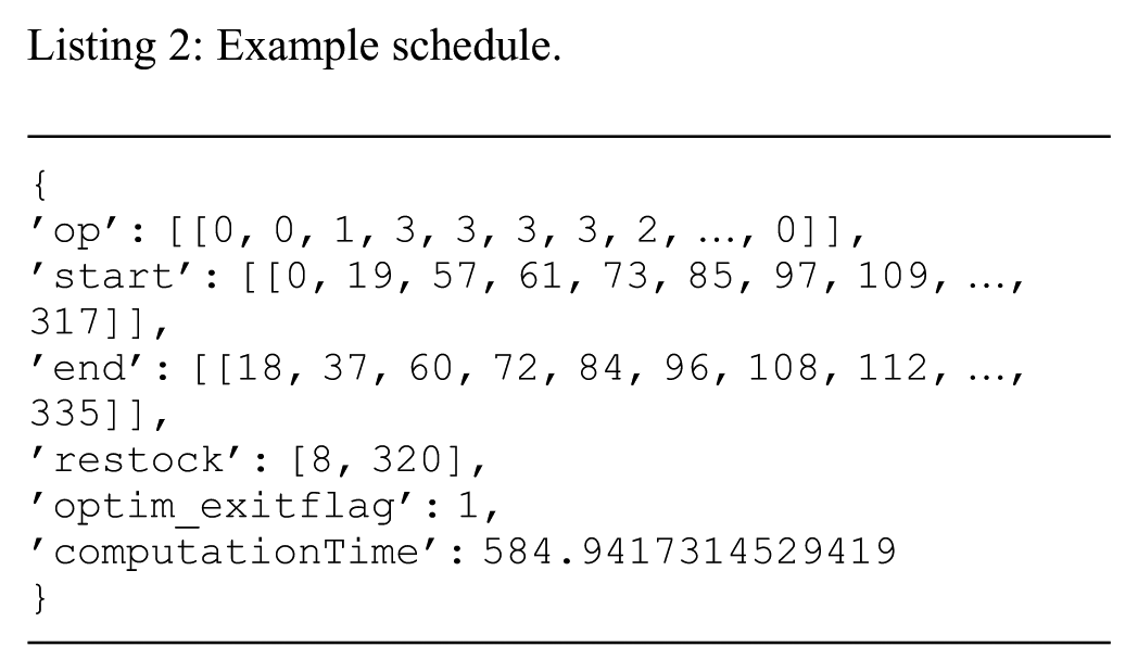
The postprocessing module harmonizes these heterogeneous outputs by converting them into a common representation: a sequence of vessel operations with defined start and end times. This standardized format enables seamless interaction with the simulation module, allowing direct comparison of results from different methods. Postprocessing is, therefore, a key enabler of the framework’s flexibility and interoperability.

In summary, the framework combines modular simulation and decision-support capabilities into a coherent, interoperable environment for offshore wind installation planning. Clearly separating the definition of scenarios, simulation, decision methods, and postprocessing ensures transparency and extensibility. Researchers can integrate and benchmark alternative approaches within a common structure, while practitioners benefit from standardized outputs that support reliable analysis and informed decision-making. Ultimately, this modular design lays the groundwork for future extensions, such as the inclusion of additional uncertainty sources, more advanced decision strategies, or real-world process monitoring data.

6. Numerical examples and results

This section presents the results of various experiments and examples that utilize the described framework to verify and validate MILP models, as well as those that employ complementary strategies to solve the offshore scheduling problem. Considering verification and validation, this section first presents a demonstrative use case for a small job-shop scheduling problem (JSSP), before presenting a more complex application in the area of offshore scheduling. Considering the decision manager, this article presents two simulation studies. The first study compares the three implemented scheduling methods against each other in isolation, while the second study explores the potential of combining these methods.

6.1. Iterative verification and validation framework

6.1.1. Functionality: JSSP

First, we use the well-known JSSP as an example to demonstrate how the proposed iterative framework (Section 4) can be used actively for verification and validation.

The JSSP is known as an NP-hard problem. By definition, a set of jobs must be executed by a set of machines in a specific order for each job. Each job has a defined execution time for each machine and a defined processing order of machines. In addition, each job must use each machine only once. The machines can execute only one job at a time, and once started, they cannot be interrupted until the assigned job is completed. The objective of this problem is to minimize the makespan, that is, the maximum completion time among all jobs. For demonstration purposes, we follow the MILP formulation of the JSSP proposed in the work by Manne.⁶⁵

The JSSP has the following input data:

$M$ : the set of machines, that is:

M = (M_{1}, \dots, M_{i}, \dots M_{n}) \in R^{n};

$J$ : the set of jobs, that is:

J = {J_{1}, \dots, J_{k}, \dots J_{m}} \in R^{m};

$o_{r}^{k}$ : the machine that processes the r th operation of job $J_{k}$ . Each job $J_{k}$ follows a processing sequence:

(o_{1}^{k}, o_{2}^{k}, \dots, o_{| O^{k} |}^{k})

where $| O^{k} |$ denotes the number of operations in Job $J_{k}$ .

$t_{ik}$ : non-negative integer processing time of job $J_{k}$ in machine $M_{i}$ .

A JSSP solution must respect the following constraints: (1) All jobs $J_{k}$ must be executed following the sequence of machines given by $O^{k}$ . (2) Each machine can process only one job at a time. (3) Once a machine starts a job, it must be completed without interruptions. The objective is to minimize the makespan, that is, the end of the last job to be executed. The JSSP is NP-hard for any fixed $m \geq 3$ and also for any fixed $n \geq 3$ . Decision variables are defined as follows.

$x_{ik}$ : starting time of job $J_{k} \in J$ on machine $M_{i} \in M$ ;

$y_{ikl} = {\begin{matrix} 1, & if job k precedes job l on machine i \\ 0, & otherwise \end{matrix}$ ;

$C$ : variable for the makespan.

In this example, we consider that there are three machines and two jobs, that is, $M = {M_{1}, M_{2}, M_{3}}$ and $J = {J_{1}, J_{2}}$ . The processing order for each job and the execution time on each machine are given as follows:

Job $J_{1}$ : $(M_{3}, 3) \to (M_{1}, 2) \to (M_{2}, 4)$ ;

Job $J_{2}$ : $(M_{2}, 2) \to (M_{3}, 3) \to (M_{1}, 5)$ .

Following an MILP formulation for the problem described above, we obtain the following:⁶⁵

min: C

s.t.:

$x_{o_{r}^{k}, k} \geq x_{o_{r - 1}^{k}, k} + t_{o_{r - 1}^{k}, k} \forall k \in J, r = 2, \dots, | O^{k} |$

$x_{ik} \geq x_{il} + t_{il} - K \cdot y_{ikl}, \forall k, l \in J, k \neq l, i \in M$

$x_{il} \geq x_{ik} + t_{ik} - K \cdot (1 - y_{ikl}) \forall i, l \in J, k \neq l, i \in M$

$C \geq x_{o_{| O^{k} |}^{k}, k} + t_{o_{| O^{k} |}^{k}, k} \forall k \in J$

$x_{ik} \geq 0 \forall k \in J, i \in M$

$y_{ikl} \in {0, 1} \forall k, l \in J, i \in M$

$C \geq 0$

The objective function is calculated in the auxiliary variable $C$ . The first set of constraints is the precedence constraints, which ensure that a job on a machine is only started after the previous machine’s processing is completed. The second and third sets of disjunctive constraints ensure that only one job is processing at a given time on a given machine. The constant K must be large enough to ensure the correctness of these constraints. A valid estimate for this value can be the summation of all processing times. The fourth set of constraints ensures that the makespan value is correctly computed, and the last constraints indicate variable domains.

6.1.1.1. Verification

First, we demonstrate with this example how the proposed framework enables modelers to detect errors. From the MILP formulation, we assume that the modelers neglected constraint 1, defining the causal dependencies between operations. Despite this omission, the MILP solver still yields solutions. The PN learned from these solutions (Figure 7(a)) using the inductive algorithm reveals multiple contradictions, which are marked in Figure 7(a).

There is no causal dependency between $o_{3}^{1}$ and $o_{1}^{2}$ ,

$o_{2}^{2}$ must occur before $o_{1}^{2}$ , and

$o_{1}^{1}$ and $o_{2}^{1}$ cannot run in parallel. These contradictions suggest that modelers should incorporate the missing causal dependencies into the MILP model.

Using PNs to validate prescriptive optimization models is straightforward: PNs make the embedded causal logic explicit as an executable graph of the intended process. For large MILP formulations with thousands of variables and constraints, verification can be a complex and tedious process. Mapping a schedule to a PN yields a compact, behavior-level representation that supports visual inspection and automated checks (e.g. reachability, deadlocks, invariants, and replay-based conformance), thereby greatly easing verification.

Figure 7.

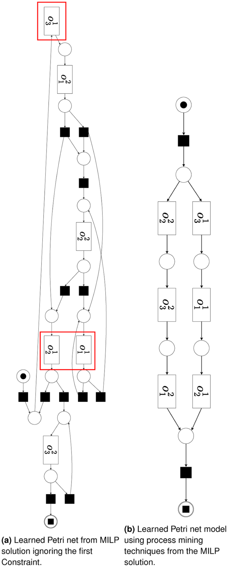
Learned Petri net models. (a) Learned Petri net from MILP solution, ignoring the first constraint. (b) Learned Petri net model using process mining techniques from the MILP solution.

6.1.1.2. Validation

The aim of validation is to assess whether the MILP schedule is consistent with a knowledge-based PN model of the domain, which we term knowledge-based validation. As in the verification example, we evaluate with respect to the makespan. The PN representation of the JSSP is shown in Figure 8.⁶⁶ Operations are modeled as stochastic transitions (here: exponential with mean equal to the nominal processing time). Machines are places; tokens encode machine availability; additional places record the status of each job.

Figure 8.

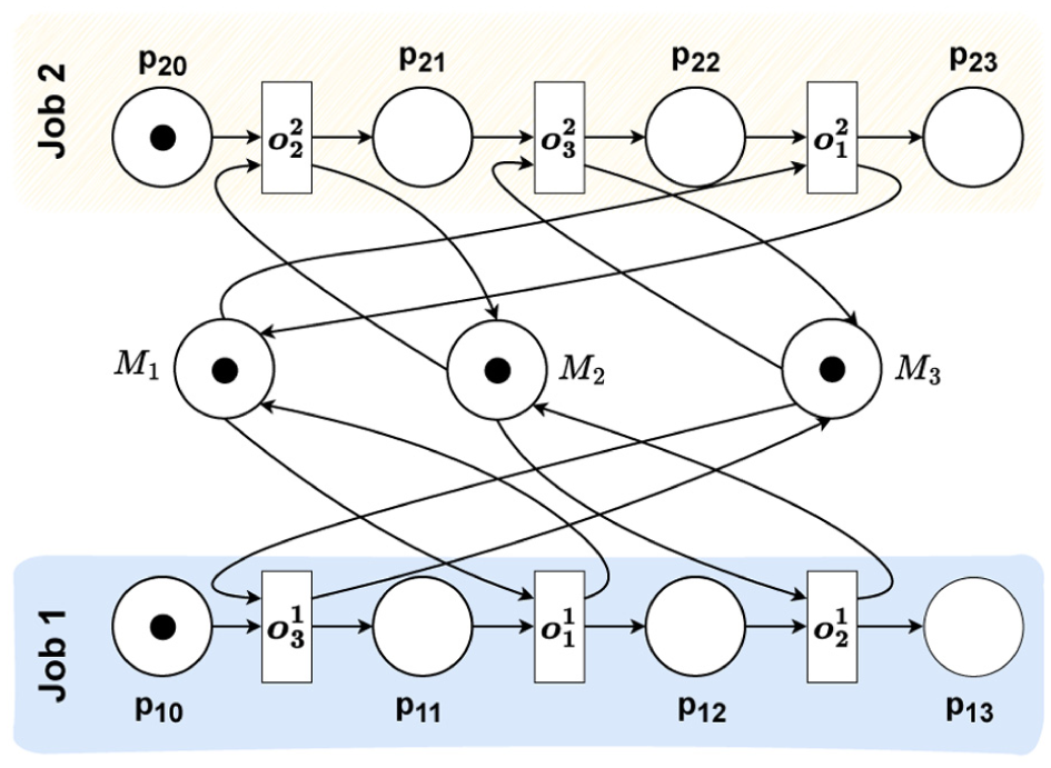
PN model for the JSSP problem.

We performed a Monte Carlo simulation with $n = 10, 000$ replications, obtained the empirical distribution of makespan, and summarized it by sample mean $\bar{x} = 11.4237$ and standard deviation $s = 5.6439$ . We then reported percentile bands at 5%, 50%, and 95% (see Figure 9); the orange dashed line marks the MILP makespan. If this value lies within the $5 %$ CI, we accept MILP as validated at the predictive level of 95%; otherwise, we report a mismatch for review. Figure 6b shows the PN derived from the validated MILP solutions, capturing the causal dependencies and the concurrency between jobs 1 and 2.

Figure 9.

Data illustration and confidence intervals.

6.1.2. Cross-model validation: OWF installation

In this work, we try to validate our models in the following three ways:

Cross-model validation of the models and event logs obtained in the same year (within year);

Cross-model validates the models and event logs obtained in different years, that is, data obtained from 2000 are tested on models derived from 2004 and vice versa (cross-year);

Knowledge validation, that is, event data, is tested on the general TPN model.

6.1.2.1. Cross-model validation (within year)

The concept of cross-model validation is illustrated in Figure 10. For each monthly scenario, we construct an event log from incumbent MILP solutions and learn a PN using inductive miner.⁶⁷

Figure 10.

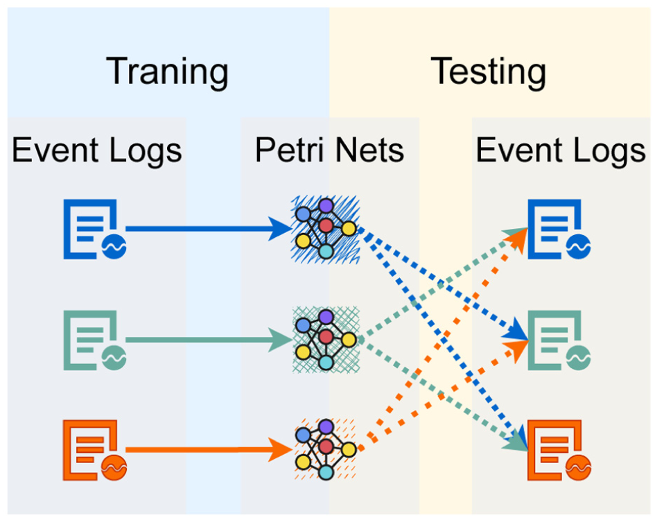
Cross-model validation.

A key aspect of the event log construction is that each log is not only derived from a single optimal MILP schedule but also from a set of incumbent (i.e. feasible but not necessarily optimal) solutions recorded during the MILP search. Each incumbent corresponds to one execution trace, and the resulting event log, therefore, captures a small set of alternative feasible process realizations.

In practice, the number of such traces per monthly instance is relatively small (typically 10–20 sequences, without timing information). This is sufficient because we abstract from temporal offsets and focus solely on the ordering relations between activities. As a result, moderate variability across incumbents does not introduce problematic noise for the inductive miner, which is known to be robust to infrequent behavior.

However, if the MILP were to generate highly diverse solutions (e.g. due to weak objective guidance or large feasible regions), the resulting log could become unstable, leading to overly complex models with many branching structures and no dominant behavior. In such cases, a restriction to the top-k incumbents (e.g. best objective values) would provide a straightforward mechanism to control noise and ensure model stability.

Each event log is then replayed on all learned PNs, and the resulting log-fitness scores are recorded. Figure 11(a) and 11(b) shows the corresponding heatmaps for the years 2000 and 2004, respectively, where the rows indicate the PN trained in a month and the columns indicate each event log. As expected, the diagonal cells are equal to or very close to 1, indicating that each PN reproduces the behavior in which it was trained.

Figure 11.

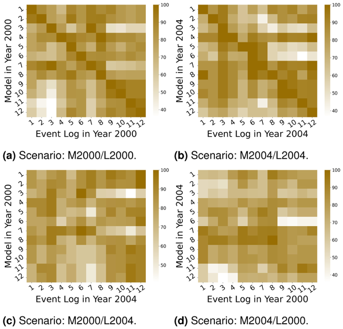
Numerical results: fitness of cross-validations. (a) Scenario: M2000/L2000. (b) Scenario: M2004/L2004. (c) Scenario: M2000/L2004. (d) Scenario: M2004/L2000.

The off-diagonal structure reveals generalization: high values indicate that a PN captures behavior beyond its own training month. In 2000 (Figure 11(a)), the months from September to December form a clear cluster with high internal fitness and lower external fitness, reflecting a seasonal separation between winter and summer behaviors. March differs across years: in 2000, the March log attains comparatively low fitness against most PNs, whereas in 2004, it fits substantially better. This contrast aligns with the process cost and duration in Figure 12: in 2000, March exhibits a lower cost/duration than April, while the opposite holds in 2004; overall levels are markedly higher in 2004. These conditions also explain the poor generalization of the PN trained in December 2004 (last row in Figure 11(b)), whose behavior appears atypical relative to other months.

Figure 12.

Cost and duration.

6.1.2.2. Cross-model validation (cross-year)

The cross-year transfer is visualized in Figure 10(c) and 10(d), where monthly event logs from 1 year are replayed on PNs learned from another year (rows: training month; columns: log month). The results indicate that offshore behavior is not homogeneous across years: for instance, the April 2004 log aligns more closely with the PN trained on May (in the same year) than with April 2000, suggesting year-specific regime differences. Despite this, seasonal structure persists. In Figure 11(c), PNs trained in September–December 2000 show consistently high fitness on late-year logs from 2004, forming a winter cluster; analogous summer blocks are also visible, albeit less pronounced.

Beyond visual clusters, two quantitative features stand out. First, cross-year transfer is asymmetric: the average fitness of 2004 logs on 2000 PNs (matrix $M 2000 \to L 2004$ ) differs from that of 2000 logs on 2004 PNs ( $M 2004 \to L 2000$ ). This asymmetry points to concept drift and changes in operating constraints or weather regimes between the 2 years. Second, the same-month correspondence is not consistently maximal across years (e.g. April ↔ April), indicating that intra-annual seasonality is a stronger predictor of transferability than calendar month alone.

These numerical patterns cohere with process-level outcomes reported elsewhere (cost/duration): months with harsher conditions in 2004 exhibit lower outbound transfer (i.e. their PNs generalize poorly to other months) and lower inbound transfer (i.e. logs from those months fit fewer external PNs). In particular, the PN trained on December 2004 shows a weak generalization to non-winter logs (last row in Figure 10(d)), suggesting a behavior profile that is atypical outside that regime.

6.1.2.3. Practical implication

Cross-year validation supports a season-aware selection policy in the decision manager: prefer PNs trained on months within the same seasonal block as the target log; fall back to year-local neighbors when cross-year fitness drops below a threshold (e.g. $< 0.8$ ). When asymmetry is high, re-learn or adapt the PN (e.g. by enriching with year-specific variants) before deployment.

6.1.2.4. Knowledge-based validation

As a sanity check, we replay each event log in the unfolded TPN in Figure 13(a). By construction, the unfolding (occurrence net) enumerates all firing sequences admissible under the scenario assumptions (single installation vessel; capacity four). Consequently, all replay-fitness scores are equal to 1, and the languages of the learned PNs are included in the TPN language $⋃_{i} L ({TPN}_{i}) \subseteq L (TPN)$ .

Figure 13.

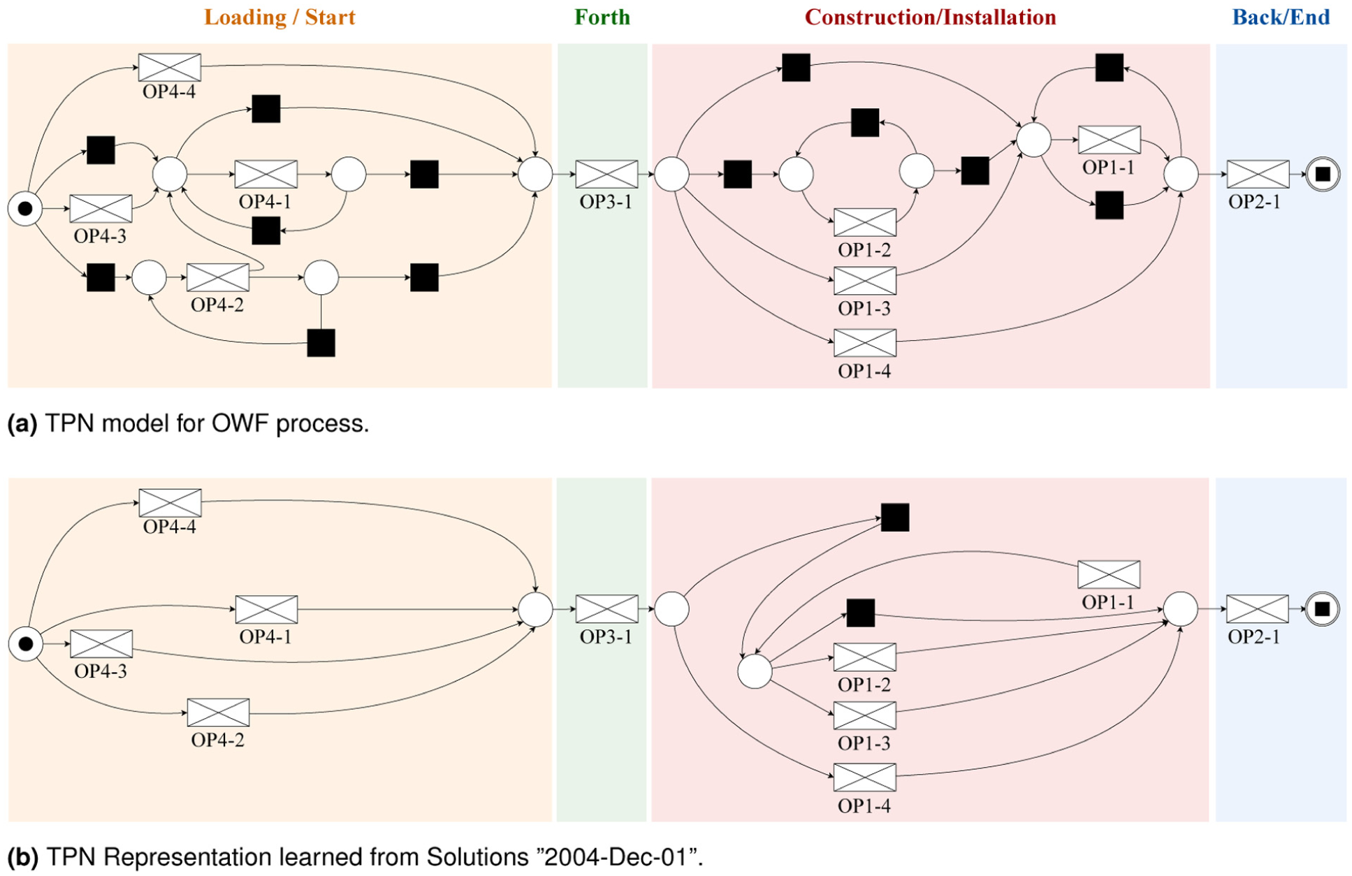
TPN models for the OWF installation process. (a) TPN model for the OWF process. (b) TPN representation learned from solutions “2004-Dec-01.”

This shows that no behavior produced by the MILP schedules violates the domain rules encoded in the TPN; hence, the MILP and TPN are consistent with domain knowledge.

6.1.2.5. Interpretation and caveat

In general, fitness $= 1$ is necessary but not sufficient: because the unfolded TPN is deliberately permissive, the result can be vacuous (high fitness may arise simply because the TPN language is a strict superset of observed behavior). The following techniques could be used to complement fitness:

precision/generalization (e.g. alignment-based precision or conformance) to penalize over-general models;

structural checks (P-/T-invariants, traps/siphons) to verify capacity and flow-conservation constraints; and

timed conformance, comparing observed sojourn times and makespan percentiles with the TPN’s timing parameters.

To complement replay fitness, we additionally computed precision for the knowledge-based validation as shown in Figure 14. While high fitness confirms that all observed MILP-derived traces are admissible under the unfolded TPN, precision evaluates the extent to which the model may still overgeneralize beyond the logs. The precision heatmaps show consistently moderate to high values across all settings, typically between about 0.6 and 0.85, with visible structure rather than random or uniformly weak scores. This suggests that, although the unfolded TPN remains deliberately permissive, the validation result is not purely vacuous. Thus, fitness and precision together provide a more informative interpretation of the knowledge-based validation by combining admissibility with an indication of behavioral specificity.

Figure 14.

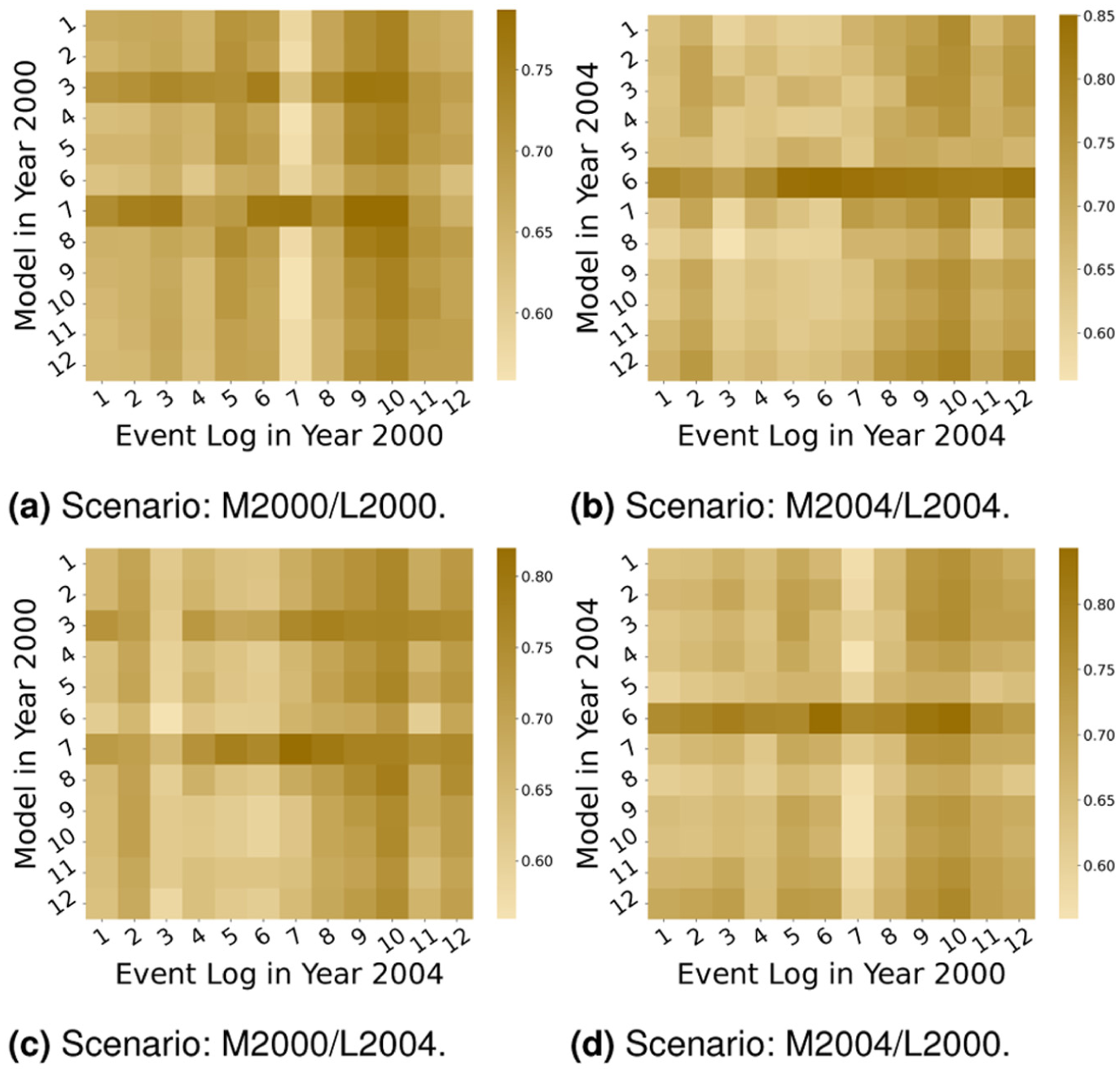
Numerical results: precision of cross-validations. (a) Scenario: M2000/L2000. (b) Scenario: M2004/L2004. (c) Scenario: M2000/L2004. (d) Scenario: M2004/L2000.

6.1.2.6. Summary

With cross-validations and knowledge-based validation, we provide evidence to support the assumptions taken in the early works.^47,68 Furthermore, with knowledge-based validation, we demonstrate that the two models share the same language, despite their fundamental differences in their formalisms.

Furthermore, with 95% confidence, a model discovered in a single month will reproduce between 75.42% and 80.19% of the behavior observed in a different month. The general standard deviation is ± 0.13, resulting from the high variation in system behavior across different seasons, which indicates a good generalization of the model.

6.1.3. Complexity discussion

The complexity of learning PN models from the event log depends on the discovery algorithm applied. In this work, the inductive miner is used.⁶⁷ The worst-case theoretical complexity is $O (n \times m^{2})$ , where n is the number of events and m is the number of unique activities.⁶⁷

However, obtaining the data logs requires executing the MILP model several times. In the case of this article, the model represents a time-indexed flexible JSSP. Such problems generally belong to the class of NP-hard or even NP-complete problems. Consequently, increasing the dimensions of the problem, in this case with respect to the planning horizon or the number of vessels, drastically increases the computational requirements.

6.1.3.1. Scalability considerations and limitations

While the theoretical complexity of both the MILP and the process discovery step can be characterized, a systematic empirical scalability analysis is beyond the scope of this work. In particular, the interaction between (1) the number of recorded incumbents, (2) the size of the resulting event logs, and (3) the complexity of the discovered PNs (e.g. in terms of places, transitions, and reachable states) has not been studied in a controlled manner.

In the present setting, scalability is not a limiting factor due to the relatively small log sizes (10–20 traces per instance) and the restricted activity set. However, for larger planning horizons, multiple vessels, or more flexible routing options, both the MILP search space and the complexity of the discovered models are expected to grow significantly.

A systematic investigation of scalability, including the impact on discovery time, model complexity, and conformance checking (e.g. reachability graph construction), is an important direction for future work.

6.2. Simulation study and comparative results for the decision manager

To demonstrate how the proposed framework supports practical planning, two simulation experiments are conducted. Together, they assess both individual and combined performance of the three scheduling methods (optimization-based, heuristic, and PN/simulation).

The first experiment compares the three methods across several representative offshore installation scenarios. It evaluates each method in isolation, establishing their performance profiles, cost, time, and computational demand, under dynamic weather conditions. These results provide a baseline understanding of each method’s strengths and weaknesses. The second experiment builds on this baseline by testing the iterative and combinatory features of the decision manager. Instead of isolating methods, it explores how sequences and combinations of them interact across successive planning cycles. This enables analysis of optimal method mixtures and identification of conditions under which hybrid strategies outperform any single approach.

6.2.1. Single scheduling method

The reference setup models the installation of 50 offshore wind turbines in Germany’s Northern Sea using a single installation vessel with a maximum transport capacity of four turbine sets, operating from the port of Eemshaven, Netherlands. The study employs a fully factorial design, combining each of the three scheduling methods with two alternative approaches to weather forecasting (see Rippel et al.³¹ for details) and six different project start dates, spanning from April to September 2000. This setup ensures that the results capture a broad spectrum of weather conditions, allowing for a systematic comparison of how each method performs under varying environmental and operational conditions.

Table 5 in Appendix 4 presents the performance metrics of three scheduling methods, mathematical optimization, heuristic, and PNs, each applied to the described project across different starting months and weather forecasting techniques. For each configuration, the table lists the number of plans required, total and per-turbine offshore time and cost, the completion hour, computational time expended, and the frequency of operational delays or missed operations.

6.2.1.1. Key findings

The experimental results demonstrate a trade-off between computational time and solution quality among the evaluated scheduling methods. The mathematical optimization method consistently achieved the lowest project costs, offshore times, and required number of installation plans across all weather conditions and months. However, this superior performance came at the expense of dramatically increased computational time, often reaching several thousand seconds per scenario. In contrast, the heuristic approach produced near-instant results but exhibited significantly higher costs and offshore times, particularly under challenging weather conditions, most evidently in April and September. The PN-based method offered an intermediate option. It is worth noting that the optimization model achieves optimal solutions for 65 of 75 plans using the Markov estimator and 61 of 78 plans using the sliding window model. The optimizer was unable to prove optimality for the other plans within the 15-min time limit (900 s).

The weather modeling method had a significant impact on performance outcomes, particularly in months with adverse weather conditions. Using a Markov chain for weather simulation generally led to greater outcome variability and a higher frequency of missed operations. The sliding window weather heuristic enhanced the robustness of scheduling, substantially reducing missed operations and improving planning performance, especially for PNs. For the mathematical optimization and heuristic approaches, the weather modeling method had a smaller but noticeable impact on overall project costs and schedule robustness. In particular, the heuristic approach shifted errors from operations taking longer during execution than in planning to operations finishing faster, showing a more conservative, or robust, duration estimation.

The results reveal pronounced seasonal effects on project performance. In favorable weather months, such as July and August, all approaches converge toward similar cost and time outcomes, making fast heuristic methods attractive for practical applications within these windows. In contrast, for months characterized by worse weather (April and September), both the heuristic and PN-based methods required significantly more plans, incurred increased costs and offshore durations, and, in the case of PNs with stochastic weather, experienced more frequent scheduling disruptions. In particular, the performance gap between methods widened when dealing with these more challenging conditions.

A key aspect highlighted by the results is the variation in the number of plans each approach generates. While the PN-based model may lag behind heuristic and mathematical optimization in terms of cost and offshore time, it consistently requires fewer plans to complete the project compared with the heuristic approach. This observation suggests that the PN method generates longer and more comprehensive plans, which require less frequent replanning in response to operational disruptions or changes in weather conditions.

Fewer plans translate to greater planning stability and potentially simpler project management, as stakeholders face less frequent schedule updates and can make longer-term commitments to resources and logistics. In contrast, relying on more frequent plan adjustments, the heuristic approach may yield higher flexibility but at the expense of predictability and possibly higher coordination overhead. Thus, despite its slightly higher costs and offshore times, the PN-based approach fosters more stable project execution with reduced replanning effort, especially relevant for complex installations where schedule reliability is as critical as cost efficiency.

6.2.1.2. Implications

The analysis highlights a clear trade-off between solution quality, computational efficiency, and planning stability. Mathematical optimization consistently yields the lowest costs and shortest times but requires substantial computational effort, making it ideal for critical projects or those involving adverse weather conditions. Heuristic methods are extremely fast and suitable for favorable weather months, although at the expense of higher costs and more frequent replanning. PN-based approaches offer a balanced alternative, providing stable plans with moderate computational requirements, which is particularly valuable when schedule reliability is as important as cost efficiency.

6.2.2. Mixed scheduling method

The second experiment evaluates the decision manager’s performance when scheduling methods are combined dynamically. To maintain tractability, the scenario models 25 turbines, corresponding to roughly a 1-month installation period. This reduction is necessary because the number of possible method sequences grows exponentially: starting from three initial plans, the combinations expand to $3^{2} = 9$ , $3^{3} = 27$ , and ultimately 18,724 distinct solution paths.

6.2.2.1. Key findings

Performance is assessed based on the number of plans, project duration in hours, variable costs in euros, the number of critical planning errors, and total computational time in seconds. Critical planning errors occur when an operation is completed faster or takes longer than expected, causing the vessel to miss subsequent operations. Table 2 summarizes the range of observed outcomes.

Table 2.

Key results of the mixed-method experiment.

Parameter	Min	Max	Mean
Num. Plans	6	14	9.9
Proj. Dur. (h)	944	1309	1027.7
Cost (€)	1,229,400	1,897,200	1,513,626
Crit. Errors	0	8	2.7
Comp. Time (s)	0.15	4039.27	1069.78

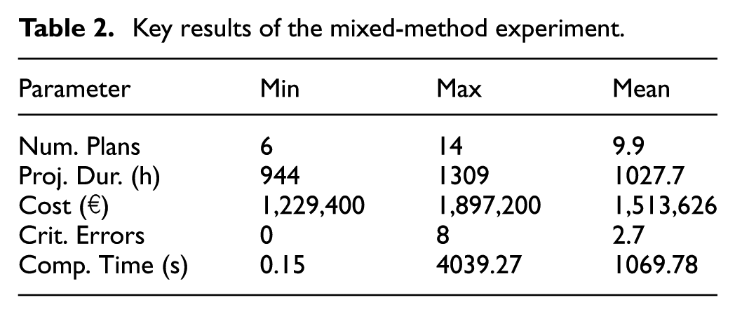
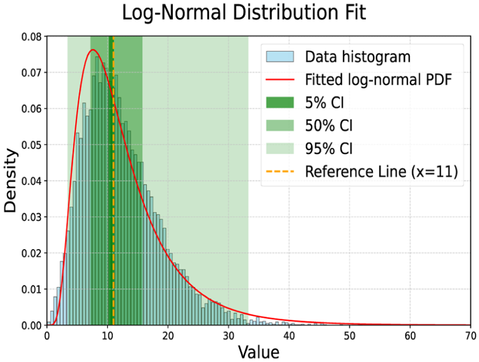
Figure 15 shows the distribution of each indicator. Except for the project duration, most indicators approximate normal distributions, slightly skewed to the left, as indicated by their mean values. This type of shape suggests that most method combinations yield viable schedules, with only a subset producing notably better or worse outcomes. Nevertheless, the span of 365 h in project duration and 668,000€ in variable costs demonstrates the substantial impact of sequence selection on planning quality.

Figure 15.

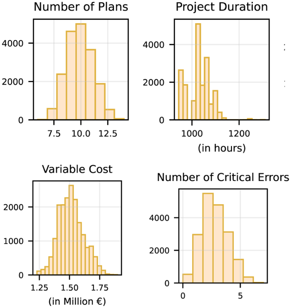
Distribution of results for each key performance indicator.

Figure 16 displays the linear correlation between indicators. Correlations remain generally low, except for the relationship between the number of plans and project duration. Interestingly, the weak correlation between project duration and costs suggests that the methods effectively mitigate offshore delays, avoiding unnecessary time in port.

Figure 16.

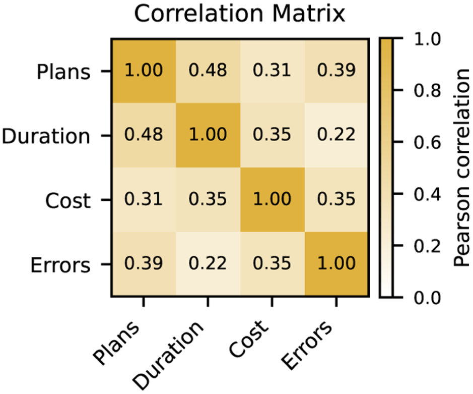
Correlation between key performance indicators.

6.2.2.2. Pareto analysis

Figures 17 and 18 visualize Pareto fronts for project duration, variable costs, and critical errors, omitting the number of plans as duration partially reflects this metric. To maintain readability, only the top 1.5% of non-dominated points are shown. All Pareto fronts were computed using NumPy’s Pareto function, minimizing all criteria.

Figure 17.

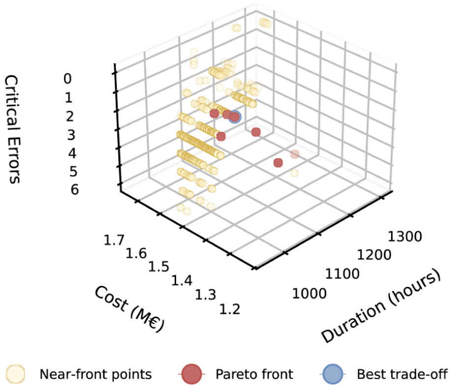
Three-dimensional Pareto front as trade-off between duration, cost, and errors.

Figure 18.

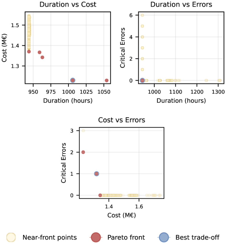
Two-dimensional Pareto fronts for all combinations of key performance indicators.

The 3D front shows that most Pareto solutions exhibit comparably low costs and durations, while allowing for some planning errors. In contrast, the 2D fronts exhibit quite classical Pareto shapes, with the front located in a concave shape along the lower left part of the plots. Remarkably, the front-end calculated only the project duration versus the number of critical errors and provided only a single solution indicated by the rectangular shape.

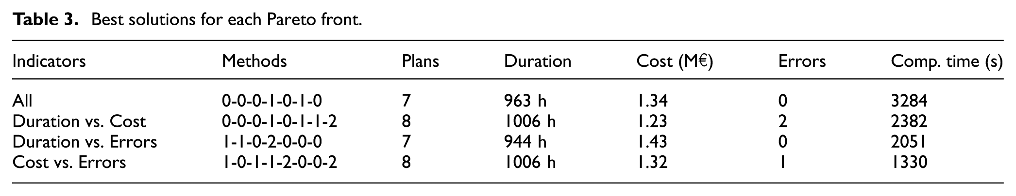
Table 3 displays the best trade-offs determined by the Pareto analysis for all three and each combination of two key performance indicators. The column Methods shows the combination of methods used during the simulation that resulted in this particular solution. The table shows that each of the best trade-offs consists of either seven or eight plans, staying on the shorter side but not achieving the minimum planning effort of six plans. As indicated by the selection of methods, most computational efforts fall within the middle area, ranging from 1330 to 3284 s to complete the entire simulation run. Interestingly, none of the best trade-offs relies on a single scheduling method, even though the computational time was not one of the key performance indicators. While three of the four solutions predominantly consist of optimization (Method 0) runs, most solutions also include (1) heuristic and (2) PN-based schedules.

Table 3.

Best solutions for each Pareto front.

Indicators	Methods	Plans	Duration	Cost (M€)	Errors	Comp. time (s)
All	0-0-0-1-0-1-0	7	963 h	1.34	0	3284
Duration vs. Cost	0-0-0-1-0-1-1-2	8	1006 h	1.23	2	2382
Duration vs. Errors	1-1-0-2-0-0-0	7	944 h	1.43	0	2051
Cost vs. Errors	1-0-1-1-2-0-0-2	8	1006 h	1.32	1	1330

6.2.2.3. Implications

These results underscore that method complementarity is both conceptual and performance-relevant. Allowing the decision manager to alternate or blend methods produces superior trade-offs between cost, reliability, and duration. Key takeaways include the following:

Dynamic orchestration: Rather than selecting one “best” scheduling algorithm, operational systems should adaptively switch methods as project conditions evolve (e.g. using fast heuristics for short-term changes and optimization for re-evaluation under stable conditions).

Performance tuning: The hybrid approach exposes levers (sequence length, switching frequency) that can be tuned to balance computational resources against scheduling quality.

System design principle: The decision manager enables systematic exploration of method portfolios, paving the way toward automated “meta-schedulers” that learn which combinations work best for given weather or resource contexts.

Managerial interpretation: Practitioners can treat scheduling not only as a static decision but also as a controllable strategy: combining precision, transparency, and responsiveness through tailored method blending.

6.3. Generalization

Although this article focuses on OWF installation, both the iterative verification–validation loop and the complementary decision-support framework were deliberately designed to be domain-agnostic. Their methodological core relies on clear interfaces, standard data representations, and normative verification principles. Accordingly, they can be re-instantiated with minimal adaptation in other domains involving resource-constrained, time-critical, and uncertainty-affected scheduling.

From a methodological perspective, the iterative verification–validation procedure offers a generic protocol for improving the transparency and trustworthiness of prescriptive optimization models. MILP solutions are converted into event logs and are translated into compact PNs. These PNs are finally evaluated through language inclusion, token replay fitness, and structural analyses, such as reachability, liveness, and boundedness. These checks apply in any application that can express resources, precedence, and timing, and where a knowledge-based PN can serve as a behavioral reference. The protocol of scenario design, solution generation with logging, and PN discovery with language comparison can be applied to new settings, such as manufacturing cells, port logistics, and clinical scheduling, by re-instantiating the scenario ontology and timing assumptions while maintaining the validation mechanics unchanged.

Similarly, the decision-support architecture allows generalization, as it separates the content of a decision model from the logic governing its selection and orchestration. The use of standardized descriptors, service interfaces, and unified schedule formats allows the framework to register heterogeneous models and to operate across multiple environments. This modularity allows for the description and application of methods, regardless of whether they originate from mathematical optimization, heuristic approaches, simulation, or data-driven learning. Furthermore, the architecture enables the dynamic selection of these methods according to contextual conditions, such as forecast quality, time to decision, or computational budget.

7. Conclusion and future work

This paper has introduced frameworks using complementary application strategies that address two long-standing gaps in OWF installation planning: (1) lack of formal verification and validation for prescriptive optimization models and (2) absence of a systematic mechanism for context-sensitive method selection. The proposed approach integrates an iterative verification–validation framework, in which feasible MILP schedules are transformed into PNs and checked against knowledge-based reference models. In addition, it incorporates a modular decision-support framework that selects and combines MILP, heuristic, and PN-based schedulers based on forecast reliability, computational budget, and required response time.

Simulations across multiple installation scenarios confirm three clear trade-offs. First, MILP optimization achieves the minimum cost but incurs high computational effort. Second, heuristics provide nearly instantaneous, but comparably short plans. Finally, PN-based scheduling yields interpretable plans at a moderate cost. The decision manager exploits these differences to create hybrid scheduling sequences that improve the overall cost–duration–robustness balance. Therefore, the framework advances both the trustworthiness of optimization models and the practical adaptability of offshore installation planning.

Future work will focus on several aspects of the framework. On one hand, the decision manager’s logic could be augmented with reinforcement learning or Bayesian optimization to adaptively infer which scheduling method or combination performs best under given weather and resource conditions. The presented experiment already provides a fully factorial data set to evaluate which decisions yielded good, moderate, or poor results for each method combination. Moreover, the focus will shift toward generalizing both approaches beyond the offshore domain by drawing generalizable conclusions and evaluating additional use cases from other domains. In addition, future work should include a systematic scalability study of the integrated MILP-process mining pipeline, particularly focusing on the trade-off between solution diversity (number of incumbents), model complexity, and conformance performance.

Footnotes

Appendix 1

Appendix 2

Appendix 3

Appendix 4 ORCID iDs

Shengrui Peng

Daniel Rippel

Funding

The authors disclosed receipt of the following financial support for the research, authorship, and/or publication of this article: The authors gratefully acknowledge the financial support of the DFG (German Research Foundation) for the project “OffshorePlan” (project number: 411010215).

Declaration of conflicting interests

The authors declared no potential conflicts of interest with respect to the research, authorship, and/or publication of this article.

Data availability statement

The codes and data used in the verification and validation experiments are available online from a public git repository https://github.com/Peng-LUH/sage-simulation-2025. In addition, provides an overview of Data Transfer Objects (JSON) used by the decision manager and exemplary API endpoints for Petri net simulations, process mining, and the simulation-based scheduling approach.

Author biographies

Shengrui Peng is a senior researcher and PhD candidate at the L3S Research Center, Leibniz University Hannover. He received his MSc in Computational Methods in Engineering in 2019 from Leibniz University Hannover. His research interests include modeling, simulation-based optimization, data and process mining, machine and deep learning, and applied artificial intelligence. He collaborates with academic and industrial partners on data-driven simulation, digital twins, and decision support for real-world operations. His email address is peng@l3s.de.

Daniel Rippel is a Senior Research Associate at BIBA—Bremer Institut für Produktion und Logistik GmbH at the University of Bremen. He holds a degree in computer science (Dipl.-Inf.) and a doctorate in engineering (Dr.-Ing.) from the University of Bremen, Germany. His research interests include modeling and simulation of logistics systems, developing domain-specific modeling methods, and integrating methods from statistics, artificial intelligence, and classic decision-making approaches. His email address is rip@biba.uni-bremen.de.

Markus Kreutz is a Senior Research Associate at BIBA—Bremer Institut für Produktion und Logistik GmbH at the University of Bremen. He obtained a master’s degree in physics from the University of Bremen, Germany. His research interests include data analysis, image processing, and the application of techniques from deep learning. His email address is kre@biba.uni-bremen.de.

Michael Freitag is a Full Professor at the University of Bremen and Director of BIBA—Bremer Institut für Produktion und Logistik GmbH. He holds a diploma degree in electrical engineering and a doctoral degree in production engineering. His research interests include modeling, simulation, and optimization of complex production and logistics systems, the development of planning and control methods for logistic processes, and the automation of physical material flows through robots and flexible transport systems. His email address is fre@biba.uni-bremen.de.

Michael Lüjten heads the Department of Data Analytics and Process Optimization at BIBA—Bremer Institut für Produktion und Logistik GmbH at the University of Bremen. He holds a doctorate in engineering and a master’s degree in production engineering from the University of Bremen. His research interests include modeling and simulation of complex production and logistics scenarios. His email address is ltj@biba.uni-bremen.de.

Helena Szczerbicka is Professor Emeritus of the Faculty of Electrical Engineering and Computer Science at the Leibniz University of Hanover, Germany. Her research interests focus on modeling, simulation, and optimization. She has served on the Board of Directors of the Society of Modeling and Computer Simulation International SCS for many years. She has received much recognition for her various scholarly publications, achievements, and professional activities that focus on the importance of modeling and simulation in its interaction with other disciplines. Her email address is hsz@sim.uni-hannover.de.

References

Peng

Rippel

Lütjen

, et al. Petri nets based iterative validation of prescriptive MILP models: a case study in offshore installation scheduling. In: The 66th international conference of Scandinavian Simulation Society, 23–24 September, Stavanger.

Peng

Szczerbicka

. A framework for iterative verification and validation of prescriptive MILP scheduling models based on Petri nets. In: 2025 annual modeling and simulation conference (ANNSIM), pp.1–13, https://ieeexplore.ieee.org/document/11118633 (accessed 23 October 2025).

Rippel

Jathe

Becker

, et al. A review on the planning problem for the installation of offshore wind farms. IFAC: PapersOnline 2019; 52: 1337–1342.

McCarl

Apland

. Validation of linear programming models. J Agri Appl Econ 1986; 18: 155–164.

Van Der Aalst

WMP

. Petri net based scheduling. Oper-Res-Spektr 1996; 18: 219–229.

Carmona

Van Dongen

Solti

, et al. Conformance checking: relating processes and models. Springer International Publishing.

Peng

Rippel

Becker

, et al. Scheduling of offshore wind farm installation using simulated annealing. IFAC: PapersOnline 2021; 54: 325–330.

Rippel

Peng

Lütjen

, et al. Model transformation framework for scheduling offshore logistics. In: Proceedings of the Hamburg international conference of logistics (HICL), pp.520–552, https://ideas.repec.org/h/zbw/hiclch/228961.html

Schwarz

Römer

Mellouli

. A data-driven hierarchical MILP approach for scheduling clinical pathways: a real-world case study from a German university hospital. Bus Res 2019; 12: 597–636.

10.

Chen

Zhang

, et al. Robustness verification of tree-based models. In Wallach

Larochelle

Beygelzimer

, et al. (eds) Advances in neural information processing systems, Vol. 32. Curran Associates, pp.12327–12337.

11.

Schrijver

. Theory of linear and integer programming. Wiley-Interscience series in discrete mathematics and optimization, Wiley, 2011.

12.

Chinneck

. Feasibility and infeasibility in optimization, international series in operations research and management science, Vol. 118. Springer US, 2008.

13.

IBM. User’s manual for cplex, 2022, https://www.ibm.com/docs/en/icos/20.1.0?topic=cplex-users-manual (accessed 21 November 2024).

14.

Gurobi. User’s manual for cplex, 2024, https://docs.gurobi.com/current/ (accessed 21 November 2024).

15.

Andersen

Boomsma

Nielsen

. MILP sensitivity analysis for the objective function coefficients. INFORMS J Optim 2023; 5: 92–109.

16.

Sargent

. A tutorial on validation and verification of simulation models. In: Proceedings of the 20th conference on Winter simulation—WSC ’88. ACM Press, pp.33–39.

17.

Pinzon

Vergara

Da Silva

LCP

, et al. An MILP model for optimal management of energy consumption and comfort in smart buildings. In: 2017 IEEE Power & Energy Society innovative smart grid technologies conference (ISGT), Washington, DC, IEEE, pp.1–5.

18.

Cheung

KKH

Gleixner

Steffy

. Verifying integer programming results. In: Eisenbrand

Koenemann

(eds) Integer programming and combinatorial optimization. Springer International Publishing, 2017, pp.148–160.

19.

Kunath

Kühn

Völker

, et al. MILP performance improvement strategies for short-term batch production scheduling: a chemical industry use case. SN Appl Sci 2022; 4: 87.

20.

Han

Peng

Shen

, et al. MILP models for flexible job shop scheduling with spatial constraints and sequence flexibility*. In: 2024 IEEE 20th international conference on automation science and engineering (CASE), Bari, IEEE, pp.2501–2506.

21.

Vis

Ursavas

. Assessment approaches to logistics for offshore wind energy installation. Sust Energ Technol Assess 2016; 14: 80–91.

22.

Muhabie

Rigo

Cepeda

, et al. A discrete-event simulation approach to evaluate the effect of stochastic parameters on offshore wind farms assembly strategies. Ocean Eng 2018; 149: 279–290.

23.

Devoy McAuliffe

Judge

Murphy

. Modelling the installation of next generation floating offshore wind farms. Appl Energy 2024; 374: 124001.

24.

Ait Alla

Quandt

Lütjen

. Simulation-based aggregate installation planning of offshore wind farms. Int J Energy 2013; 7: 23–30.

25.

González

MOA

Nascimento

Jones

, et al. Logistic decisions in the installation of offshore wind farms: a conceptual framework. Energies 2024; 17: 6004.

26.

Irawan

Wall

Jones

. An optimisation model for scheduling the decommissioning of an offshore wind farm. OR Spectrum 2019; 41: 513548.

27.

Ursavas

. A benders decomposition approach for solving the offshore wind farm installation planning at the North Sea. Eur J Oper Res 2017; 258: 703–714.

28.

Beinke

Ait Alla

Oelker

, et al. Demand for special vessels for the decommissioning of offshore wind turbines in the German North Sea: a simulation study. In: Chung

Akselsen

Jin

, et al. (eds) Proceedings of the 30th international ocean and polar engineering conference (ISOPE). ISOPE, pp.480–484.

29.

Oelker

Ait Alla

Büsing

, et al. Simulative approach for the optimization of logistic processes in offshore ports. In: Chung

Akselsen

Jin

, et al. (eds) Proceedings of the 30th international ocean and polar engineering conference (ISOPE). ISOPE, pp.446–452.

30.

Kerkhove

Vanhoucke

. Optimised scheduling for weather sensitive offshore construction projects. Omega 2017; 66: 58–78.

31.

Rippel

Jathe

Lütjen

, et al. Evaluation of loading bay restrictions for the installation of offshore wind farms using a combination of mixed-integer linear programming and model predictive control. Appl Sci 2019; 9: 5030.

32.

Rippel

Lütjen

Szczerbicka

, et al. A cascading online-simulation framework to optimize installation cycles for offshore wind farms. In: 2021 Winter simulation conference (WSC), Phoenix, AZ, 12–15 December, pp. 1–12. IEEE.

33.

Hick

Bajzek

Faustmann

. Definition of a system model for model-based development. SN Appl Sci 2019; 1: 10690.

34.

Schmidt

Zimmermann

Stark

. Systematic literature review of system models for technical system development. Appl Sci 2021; 11: 3014.

35.

Scholz -Reiter

de Beer

Freitag

, et al. Dynamik logistischer Systeme. In: Nyhuis

(ed.) Beiträge zu einer Theorie der Logistik. Springer, 2008, pp.109–138.

36.

Gils

Gardian

Kittel

, et al. Model-related outcome differences in power system models with sector coupling: quantification and drivers. Renew Sust Energ Rev 2022; 159: 112177.

37.

Henry

Eshraghi

Lugovoy

, et al. Promoting reproducibility and increased collaboration in electric sector capacity expansion models with community benchmarking and intercomparison efforts. Appl Energy 2021; 304: 117745.

38.

Schweiger

Nilsson

Schoeggl

, et al. Modeling and simulation of large-scale systems: a systematic comparison of modeling paradigms. Appl Math Comput 2020; 365: 124713.

39.

Batty

. Digital twins. Environ Plan B: Urban Anal City Sci 2018; 45: 817–820.

40.

Tuncel

Bayhan

. Applications of Petri nets in production scheduling: a review. Int J Adv Manuf Technol 2007; 34: 762–773.

41.

Murata

. Petri nets: properties, analysis and applications. Proc IEEE 1989; 77: 541–580.

42.

Zhou

Jeng

. Modeling, analysis, simulation, scheduling, and control of semiconductor manufacturing systems: a Petri net approach. IEEE Trans Semiconduct Manuf 1998; 11: 333–357.

43.

Van Der Aalst

WMP

. Process mining: discovery, conformance and enhancement of business processes. Springer, 2011.

44.

Wang

. Timed Petri nets, The Kluwer international series on discrete event dynamic systems, Vol. 9. Springer, 1998.

45.

Popova-Zeugmann

. Timed Petri nets. Springer, 2013.

46.

Peng

Szczerbicka

Becker

. Modeling and simulation of offshore wind farm installation with multi-leveled CGSPN approach. In: Proceedings of the international offshore and polar engineering conference, Virtual, Online: International Society of Offshore and Polar Engineers, pp.1–8, https://publications.isope.org/proceedings/ISOPE/ISOPE%202020/data/pdfs_Vol1/1193-20TPC-0390.pdf (accessed 23 October 2025).

47.

Peng

Rippel

Becker

, et al. Simulatin-based scheduling for offshore wind farm installation using timed Petri nets approach. In: Proceedings of the 2020 summer simulation conference, Madrid, Society for Computer Simulation International, p.12.

48.

Solé

Carmona

. Incremental process discovery. In: Jensen

Donatelli

Kleijn

(eds) Transactions on Petri nets and other models of concurrency V, Vol. 6900. Springer, pp.221–242.

49.

Bergenthum

Desel

Lorenz

, et al. Process mining based on regions of languages. In: Alonso

Dadam

Rosemann

(eds) Business process management, Vol. 4714. Springer, pp.375–383.

50.

Van Der Aalst

WMP

. Process mining. Springer, 2016.

51.

Kourani

Berti

Schuster

, et al. ProMoAI: process modeling with generative AI. In: Proceedings of the thirty-third international joint conference on artificial intelligence. Jeju, South Korea, International Joint Conferences on Artificial Intelligence Organization, pp.8708–8712.

52.

Van Der Aalst

WMP

. Process mining: data science in action. 2nd ed. Springer, 2016.

53.

Luo

Xing

Zhou

, et al. Deadlock-free scheduling of automated manufacturing systems using Petri nets and hybrid heuristic search. IEEE Trans Syst Man Cybernet: Syst 2015; 45: 530–541.

54.

Zhong

, et al. Deadlock analysis and control using Petri net decomposition techniques. Inform Sci 2019; 482: 440–456.

55.

. Robust deadlock detection and control of automated manufacturing systems with multiple unreliable resources using Petri nets. IEEE Trans Automat Sci Eng 2021; 18: 1790–1802.

56.

Esmaeeli

Aleahmad

. Bottleneck detection in job shop production by high-level Petri nets. In: 2019 15th Iran international industrial engineering conference (IIIEC), Yazd, IEEE, pp.178–183.

57.

Zeng

Liu

Duan

. Resource conflict detection and removal strategy for nondeterministic emergency response processes using Petri nets. Enterp Inform Syst 2016; 10: 729–750.

58.

Axtell

Axelrod

Epstein

, et al. Aligning simulation models: a case study and results. Comput Math Organ Theory 1996; 1: 123–141.

59.

Sargent

. Verification and validation of simulation models. J Simul 2013; 7: 12–24.

60.

Rippel

Foroushani

Lütjen

, et al. A crew scheduling model to incrementally optimize workforce assignments for offshore wind farm constructions. Energies 2021; 14: 22.

61.

Ramadge

Wonham

. Supervisory control of a class of discrete event processes. SIAM J Contr Optim 1987; 25: 206–230.

62.

Cassandras

Lafortune

. Introduction to discrete event systems. Springer, 2021.

63.

Zeigler

Muzy

Kofman

. Theory of modeling and simulation. Academic Press, 2018.

64.

Rippel

Kreutz

Lütjen

, et al. From literature to practice: taxonomy to compare system models for offshore wind farm applications. J Simul 2026; 1: 1–18.

65.

Manne

. On the job-shop scheduling problem. Oper Res 1960; 8: 219–223.

66.

Huang

Ahmad

. Job shop scheduling with Petri nets. In: Pardalos

Graham

(eds) Handbook of combinatorial optimization. Springer, 2013, pp.1667–1711, https://link.springer.com/10.1007/978-1-4419-7997-1_51

67.

Leemans

SJJ

Fahland

and Van Der Aalst WMP. Discovering block-structured process models from incomplete event logs. In: Ciardo

Kindler

(eds) Application and theory of Petri nets and concurrency, Vol. 8489. Springer, 2014. pp.91–110.

68.

Rippel

Jathe

Lütjen

, et al. Simulation and optimization of operations for offshore installations planning using a model predictive control scheme. In: 2019 Winter simulation conference (WSC), National Harbor, MD, IEEE, pp.1719–1730.