Elliptic-hyperbolic coordinates for the numerical investigation of elliptical hole problems: A finite difference solution

Abstract

An elliptical hole can cover several different defect shapes within a material, ranging from thin cracks to round holes. In this study, an elliptical-hyperbolic coordinate system was used to mesh a geometry with traction-free elliptical holes. A new transformation was applied to map the physical domain to a computational Cartesian domain, in which the finite difference technique was applied. A few test cases involving ellipses of various shapes, from an almost round hole to a crack, were analyzed numerically. They were subjected to unidirectional and bidirectional loads far away from the hole location. The numerical and exact analytical results showed a good agreement. The stress intensity factors of a central crack and an edge crack subjected to unidirectional loading were extracted by correlating the normal stress ahead of the crack tip and the vertical crack face displacement behind the crack tip using three terms of the asymptotic expansion. The accuracy of both methods was excellent, with an error <1%. The good agreement between the numerical and analytical results confirms the reliability of the proposed technique and paves the way for addressing more complex geometries and material models.

Keywords

elliptic-hyperbolic coordinates elliptical hole crack stress concentration stress intensity finite differences

1. Introduction

Elliptical holes serve as a useful model to approximate defects, inclusions, and cracks found in plate structures in civil, mechanical, and structural engineering.¹ Predicting the stress concentration owing to these holes allows engineers to prevent failure initiation and design safe components. The elliptical hole is a unifying model. When the ratio between the minor and major axes of the ellipse approaches 1, it becomes circular. When the ratio approaches 0, it degenerates into cracks. This continuous transition encompasses many optional defect shapes within a material. The problem of an infinite plate with a traction-free elliptical hole loaded at infinity was first studied by Inglis,² who derived the stress concentration factor around an elliptical hole. This problem has been studied analytically for many years by other researchers.^3–6 Such studies have provided exact analytical solutions, which have served as the standard for validating numerical methods^7,8 before addressing more complex geometries and material models. The use of an elliptic-hyperbolic coordinate system (EHCS) results in boundary conformity. The coordinates exactly match the shape of the elliptical holes, and the boundary conditions can be expressed easily and naturally because the boundary aligns with the coordinate axes.

This study aimed to check the use of an EHCS with the finite difference (FD) technique in predicting stress concentration factors (SCFs) and stress intensity factors (SIFs) due to the presence of an elliptical hole. The author is not aware of any other study that uses EHCS with FD to calculate SCFs and SIFs. The verification and validation were performed by solving various problems of traction-free elliptical holes subjected to remote uniaxial and biaxial loads and comparing them with exact analytical solutions. This study verifies the applicability and accuracy of this numerical technique.

The remainder of this paper is organized as follows. Section 2 introduces the EHCS. The meshing in the physical domain and its mapping to the computational domain are explained in Section 3. Section 4 introduces the test cases that were solved and details the meshes, boundary conditions, and results. Finally, Section 5 presents a summary and conclusions.

2. Elliptic-hyperbolic coordinate system

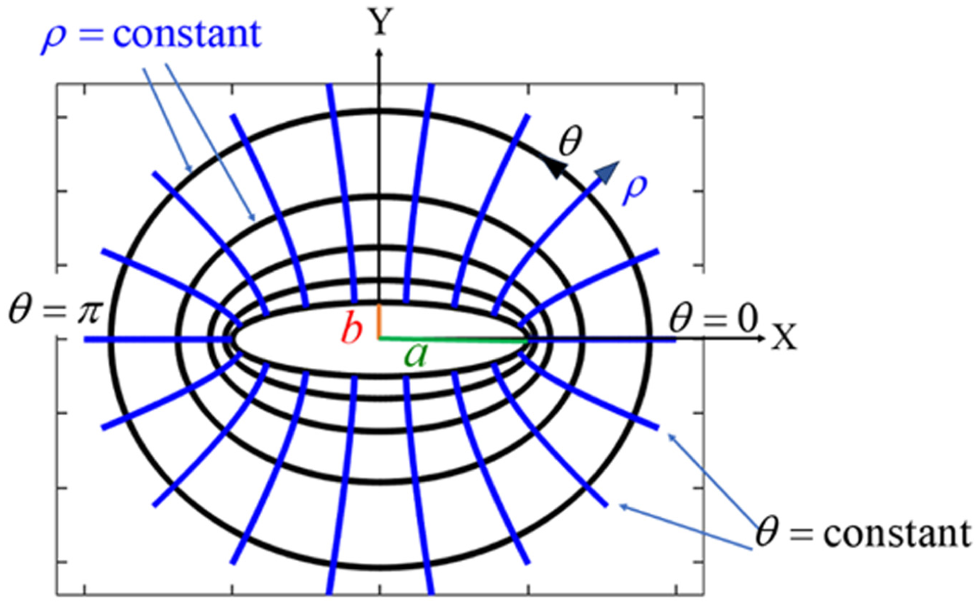
Figure 1 shows a two-dimensional orthogonal EHCS $(ρ, θ)$ around an elliptical hole, where “a” and “b” denote the semi-major and semi-minor axes of the elliptical hole, respectively.

Figure 1.

Two-dimensional orthogonal EHCS $(ρ, θ)$ around an elliptical hole.

The transformation from an EHCS to Cartesian coordinates is given by Equations 1(a)–(e). The eccentricity is c.

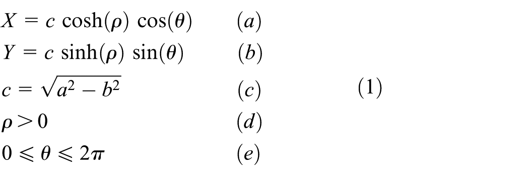
\begin{matrix} X = c \cosh (ρ) \cos (θ) (a) \\ Y = c \sinh (ρ) \sin (θ) (b) \\ c = \sqrt{a^{2} - b^{2}} (c) \\ ρ > 0 (d) \\ 0 \leq θ \leq 2 π (e) \end{matrix}

(1)

The elimination of θ from Equations 1(a) and (b) yields:

\frac{X^{2}}{{[c \cosh (ρ)]}^{2}} + \frac{Y^{2}}{{[c \sinh (ρ)]}^{2}} = 1 .

(2)

This shows that the lines of constant ρ (black color in Figure 1) are ellipses. The elimination of ρ from Equations 1(a) and (b) yields:

\frac{X^{2}}{{[c \cos (θ)]}^{2}} - \frac{Y^{2}}{{[c \sin (θ)]}^{2}} = 1 .

(3)

This shows that the lines of constant θ (blue color in Figure 1) are hyperboloids.

Explicit equations for deriving elliptic-hyperbolic coordinates from the Cartesian grid were developed by Sun.⁹ The equations are as follows:

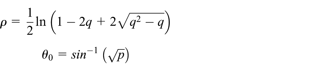
\begin{matrix} ρ = \frac{1}{2} \ln (1 - 2 q + 2 \sqrt{q^{2} - q}) \\ θ_{0} = \sin^{- 1} (\sqrt{p}) \end{matrix}

where

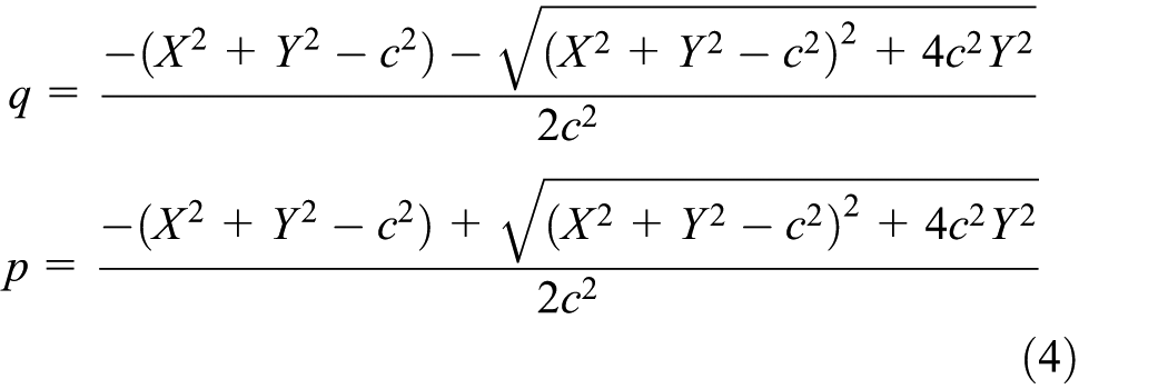
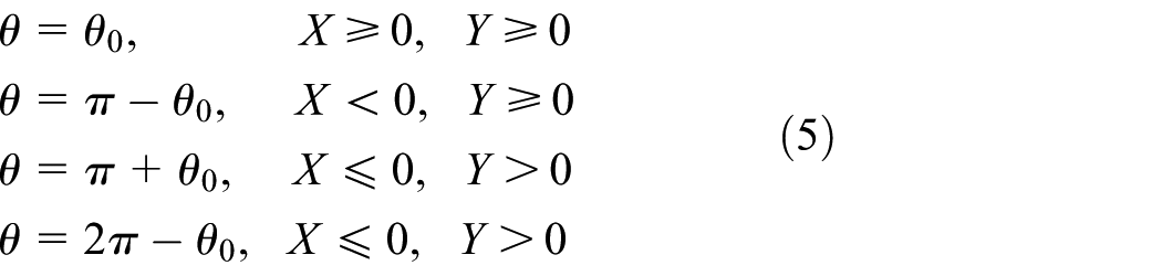
\begin{matrix} q = \frac{- (X^{2} + Y^{2} - c^{2}) - \sqrt{{(X^{2} + Y^{2} - c^{2})}^{2} + 4 c^{2} Y^{2}}}{2 c^{2}} \\ p = \frac{- (X^{2} + Y^{2} - c^{2}) + \sqrt{{(X^{2} + Y^{2} - c^{2})}^{2} + 4 c^{2} Y^{2}}}{2 c^{2}} \end{matrix}

(4)

There are four cases for the coordinate θ depending on the quadrant in which the Cartesian point (X, Y) is located:

\begin{matrix} θ = θ_{0}, X \geq 0, Y \geq 0 \\ θ = π - θ_{0}, X < 0, Y \geq 0 \\ θ = π + θ_{0}, X \leq 0, Y > 0 \\ θ = 2 π - θ_{0}, X \leq 0, Y > 0 \end{matrix}

(5)

3. FD mesh and transformation

The FD technique used herein maps the physical domain, which is meshed with an EHCS (ρ, θ), to a computational square domain using the Cartesian coordinate system (ξ, η), where $1 \leq ζ \leq 2$ and $1 \leq η \leq 2$ . The mesh size is constant in the computational domain but varies in the physical domain. Appropriate mapping can impose a dense mesh on the areas of stress concentration.

This technique has been used in Cartesian physical domains for solving crack problems, including contact and friction in homogeneous isotropic materials^10–12 and functionally graded materials.^13,14 It has also been used with polar curvilinear coordinates for Brazilian disks.¹¹ These studies fully describe the FD technique used in this study. For example, the two-dimensional (2D) displacement equilibrium equations in Cartesian coordinates and their transformed shape, in which the derivatives of the Cartesian coordinates are transformed to any curvilinear coordinate system, are detailed in the work by Dorogoy.¹³ The application of tractions and displacement boundary conditions is explained. The coefficients, which depend on the mixed derivatives of both coordinate systems at the point of application, are given explicitly in Appendix 1 of Dorogoy.¹³

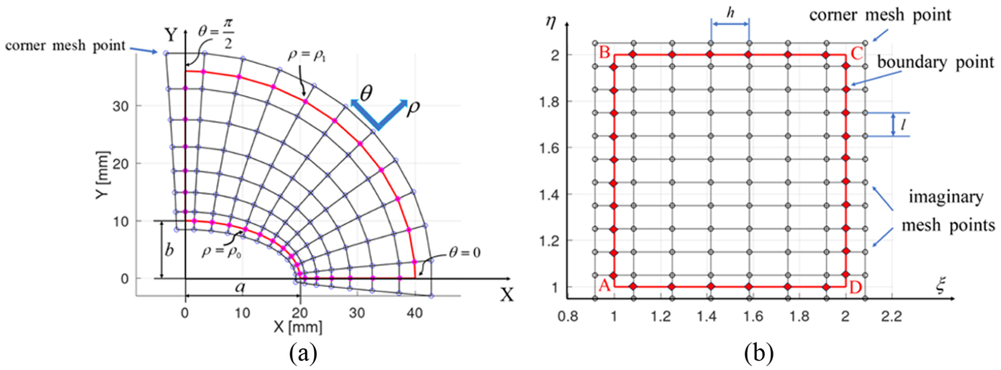
Figure 2(a) shows a typical elliptical-hyperbolic mesh in the physical domain. Here, $ρ_{0} \leq ρ \leq ρ_{1}$ and $0 \leq θ \leq \frac{π}{2}$ . Figure 2(b) shows the computational domain with the transformed (ξ, η) mesh. In this formation, the tip of the ellipse (or crack when b = 0) lies in the lower left corner, designated by the letter A in Figure 2(b).

Figure 2.

(a) Elliptical physical domain meshed with an elliptic-hyperbolic coordinate system where $ρ_{0} \leq ρ \leq ρ_{1}$ and $0 \leq θ \leq \frac{π}{2}$ . (b) Transformed mesh in the computational domain, where $1 \leq ζ \leq 2$ and $1 \leq η \leq 2$ .

A polynomial transformation is applied:

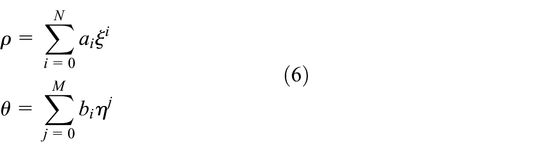
\begin{matrix} ρ = \sum_{i = 0}^{N} a_{i} ξ^{i} \\ θ = \sum_{j = 0}^{M} b_{i} η^{j} \end{matrix}

(6)

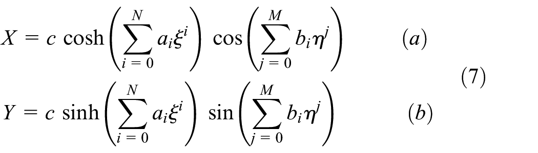
The transformation must be continuous and smoothly differentiable. A polynomial fulfills these conditions, but any other suitable function can be chosen. The transformation must be single-valued. For each value of $1 \leq ζ_{i} \leq 2,$ there should be only one value of $ρ_{0} \leq ρ_{i} \leq ρ_{1}$ . For each value of $1 \leq η_{j} \leq 2,$ there should be only one value of $θ_{0} \leq θ_{j} \leq θ_{1}$ . This condition requires the first derivatives to be positive: $\frac{d ρ}{d ζ} > 0$ in $ρ_{0} \leq ρ \leq ρ_{1}$ and $\frac{d θ}{d η} > 0$ in $θ_{0} \leq θ \leq θ_{1}$ .

Substituting Equation (6) into Equations 1(a) and (b) yields the transformation from the computational domain (ξ, η) to the physical domain (X, Y), that is,

\begin{matrix} X = c \cosh (\sum_{i = 0}^{N} a_{i} ξ^{i}) \cos (\sum_{j = 0}^{M} b_{i} η^{j}) (a) \\ Y = c \sinh (\sum_{i = 0}^{N} a_{i} ξ^{i}) \sin (\sum_{j = 0}^{M} b_{i} η^{j}) (b) \end{matrix}

(7)

4. Test cases

The new elliptic-hyperbolic transformation was verified numerically using four test cases with known analytical solutions.

Case I: An infinite elastic plate with an elliptical hole is subjected to remote uniform biaxial loading.

Case II: An infinite elastic plate with an elliptical hole is subjected to remote uniaxial loading normal to the major axis.

Case III: An infinite elastic plate with a central crack (2a) is subjected to remote uniaxial loading normal to the crack face.

Case IV: Infinite elastic plate with an edge crack (a) subjected to remote uniaxial loading normal to the crack face.

Two-dimensional plane strain analyses were conducted assuming a homogeneous isotropic material with a Young’s modulus E = 5000 N/mm² and a Poisson’s ratio of 0.3. Three freeware programs were used for the analyses.^15–17 The source code was written in Fortran 90. The Intel^® Fortran Compiler, part of the Intel^® oneAPI HPC Toolkit, was used to edit, compile, and execute the code. The large, sparse systems of linear algebraic equations resulting from the FD formulation were solved efficiently and accurately using the Y12M software package. •Y12M is written in Fortran and utilizes Gaussian elimination. These subroutines were treated as a “black box.” Finally, the results were post-processed and plotted using GNU Octave.

4.1. Meshing

The meshing for the four test cases comprised 220 mesh points in the ρ direction and 92 points in the θ direction. Because there are two unknown displacements (U and V) at each mesh point, the mesh has $2 \times 220 \times 92 = 40, 480$ degrees of freedom. The major axis of the inner ellipse/crack was 20 mm. To resemble an infinite plate, the load was applied at a distance 10a (at θ = 0). A mesh convergence study which justify the chosen mesh and the location of load application is given in Appendix 2. Because all the test cases were symmetric, only a quarter of the physical domain was analyzed. The range $ρ_{0} \leq ρ \leq ρ_{1}$ was determined using Equation (4); Table 1 presents the results. The θ range is $0 \leq θ \leq π / 2$ . The mapping of (ρ, θ) to (ξ, η) was done using a second-order polynomial:

\begin{matrix} ρ = a_{0} + a_{1} ξ + a_{2} ξ^{2} \\ θ = b_{0} + b_{1} η + b_{2} η^{2} \end{matrix}

(8)

Table 1 presents the coefficients for all the test cases. The coefficients b_i, i = 0–2 were identical for all four geometries ( $b / a$ ). The coefficients a_i, i = 0–2 were different, and the resulting meshes were similar.

Table 1.

Coefficients for mapping (ξ, η) to (ρ, θ) derived using Equation (8).

			$ρ$			$θ$
$b / a$	$ρ_{0}$	$ρ_{1}$	$a_{0}$	$a_{1}$	$a_{2}$	$b_{0}$	$b_{1}$	$b_{2}$
0	0.0	2.9932	−1.6108	0.9197	0.6912	−1.6406	1.6755	−0.0349
0.10	0.1003	2.9983	−1.0383	0.2591	0.8796	−1.6406	1.6755	−0.0349
0.25	0.2554	3.0256	−0.2736	−0.5916	1.1206	−1.6406	1.6755	−0.0349
0.50	0.5493	3.1377	0.8249	−1.7076	1.4320	−1.6406	1.6755	−0.0349
0.75	0.9730	3.4080	1.8483	−2.5305	1.6552	−1.6406	1.6755	−0.0349

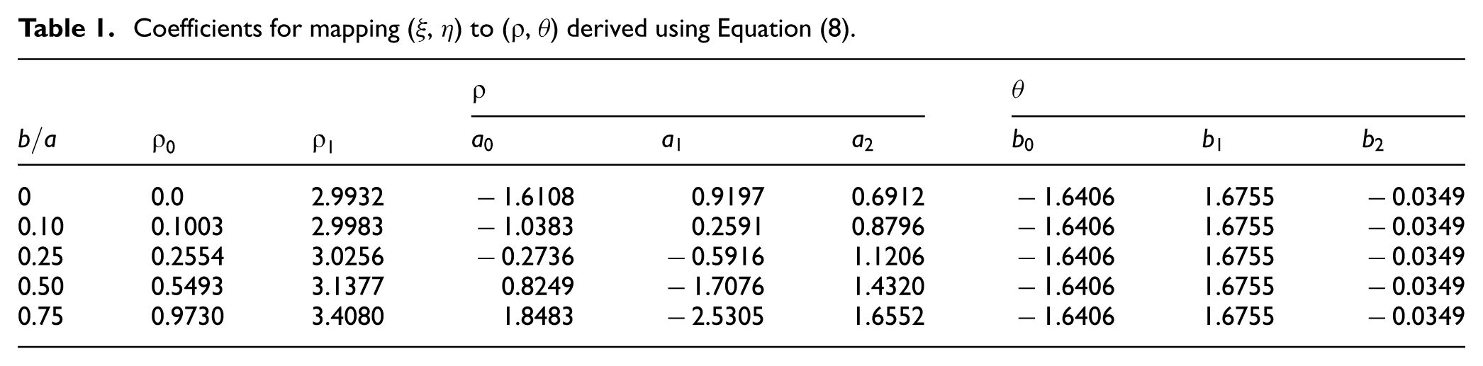
The coefficients $(a_{0}, a_{1}, a_{2})$ were calculated by solving a system of three algebraic equations.

ρ_{0} = a_{0} + a_{1} \cdot 1 + a_{2} \cdot 1^{2}

(9a)

ρ (ξ^{*}) = a_{0} + a_{1} ξ^{*} + a_{2} {(ξ^{*})}^{2}

(9b)

ρ_{1} = a_{0} + a_{1} \cdot 2 + a_{2} \cdot 2^{2}

(9c)

The parameters $ξ^{*}$ and $ρ (ξ^{*})$ are guessed through an iterative trial-and-error process until a suitable transformation is achieved. The parameters $ρ_{0}$ and $ρ_{1}$ are obtained with the usage of Equations (4) using 2 (x,y) points of the physical boundary: (b,0), (10b, 0).

A similar technique is used to obtain the coefficients $(b_{0}, b_{1}, b_{2})$ :

θ_{0} = b_{0} + b_{1} \cdot 1 + b_{2} \cdot 1^{2}

(10a)

θ (η^{*}) = b_{0} + b_{1} η^{*} + b_{2} {(η^{*})}^{2}

(10b)

θ_{1} = b_{0} + b_{1} \cdot 2 + b_{2} \cdot 2^{2}

(10c)

The parameters $θ_{0}$ and $θ_{1}$ in this study are 0 and $\frac{π}{2}$ , respectively. The parameters $η^{*}$ and $θ (η^{*})$ are guessed through an iterative trial-and-error process until a suitable transformation is achieved.

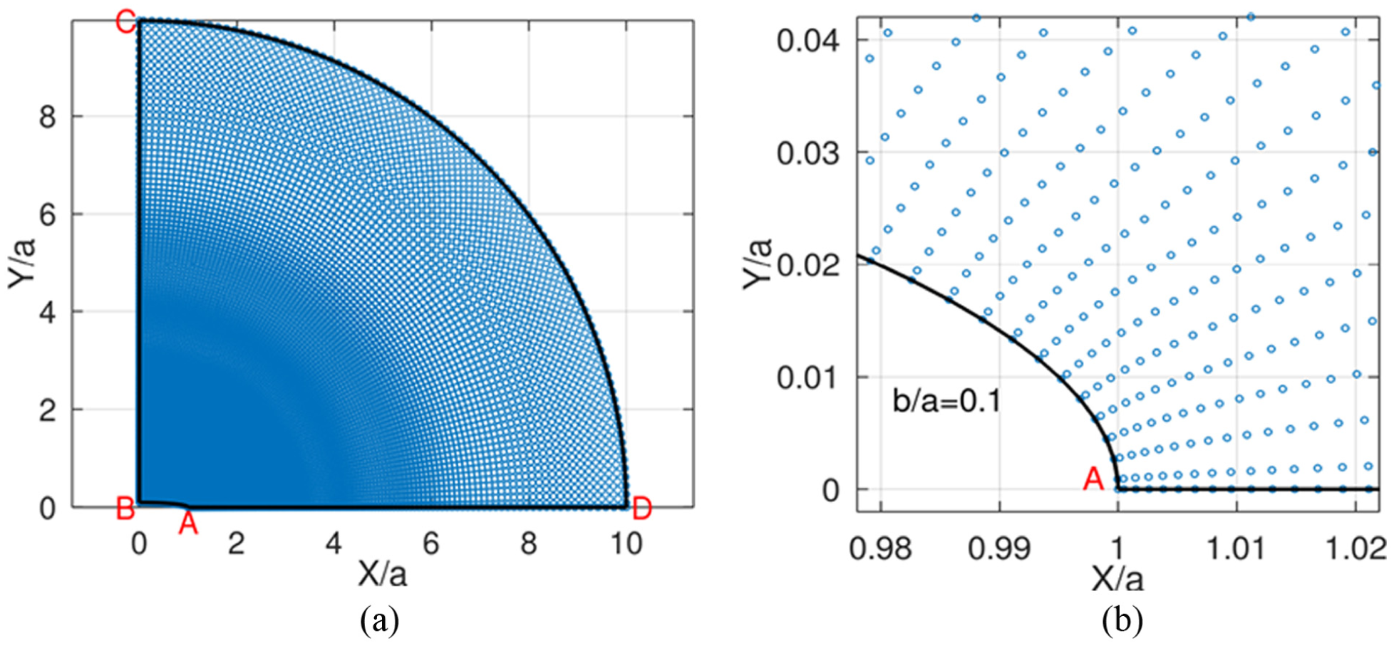
Figure 3(a) shows a mesh corresponding to the case of $b / a = 0.1$ . A zoomed-in view of the area near the ellipse/crack tip A is shown in Figure 3(b) (the ellipse becomes a crack when the minor axis b is zero). In Figure 3(b), the mesh in the physical domain is dense and unequal. It is denser near the elliptical hole and close to Tip A. The normalized distance between the mesh points at $θ = 0$ near Tip A (1 < X/a < 1.1) is between 0.1% and 0.5% of the major axis a. It reaches 17% at $ρ = ρ_{1}$ on the outer boundary $\hat{CD}$ .

Figure 3.

(a) Interior mesh for solving an infinite elastic plate with an elliptical hole under biaxial equal loading for $\frac{b}{a} = 0.1$ . (b) Zoomed-in view near Tip A, where the mesh is dense and of unequal size.

4.2. Boundary conditions

The meshed model has four faces, as shown in Figure 3(a), on which the boundary conditions are applied: the elliptical face at $ρ_{0}$ ( $\overset{⌣}{AB})$ , outer boundary during $ρ_{1}$ ( $\overset{⌣}{CD})$ , symmetry lines at $θ = 0$ ( $\bar{AD})$ , and $θ = π / 2$ ( $\bar{BC}$ ).

Figure 4 shows an elliptical hole under remote biaxial loading. The boundary conditions are applied in the (ξ, η) coordinate system of the computational domain. The (ξ, η) axes are aligned with the (ρ, θ) axes. At any point $(X_{p}, Y_{p})$ on the ellipse with constant ρ, far away from the hole, the shear stress is zero: $σ_{XY} = 0$ . The normal $\vec{n}$ is pointing in the ξ direction with an angle ϕ to the x-axis. The stresses in the (ξ, η) direction are given by:

\begin{matrix} σ_{ξ ξ} = σ_{XX} \cos^{2} ϕ + σ_{YY} \sin^{2} ϕ \\ σ_{ξ η} = (σ_{YY} - σ_{XX}) \sin ϕ \cos ϕ \end{matrix}

(11)

For the uniform biaxial load, $λ = 1$ and $σ_{YY} = σ_{XX} = S$ . The applied boundary conditions are as follows:

\begin{matrix} σ_{ξ ξ} = S \\ σ_{ξ η} = 0 \end{matrix}

(12)

For the uniaxial load, $λ = 0$ ; hence, $σ_{XX} = 0$ and $σ_{YY} = S$ . The applied boundary conditions are as follows:

\begin{matrix} σ_{ξ ξ} = S \sin^{2} ϕ \\ σ_{ξ η} = S \sin ϕ \cos ϕ \end{matrix}

(13)

The major and minor axes of the outer ellipse $ρ_{1}$ are given by:

\begin{matrix} a^{*} = c \cosh (ρ_{1}) \cos (0) = c \cosh (ρ_{1}) \\ b^{*} = c \sinh (ρ_{1}) \sin (\frac{π}{2}) = c \sinh (ρ_{1}) \end{matrix}

(14)

The slope of the normal at the point $(X_{p}, Y_{p})$ is given by:

m_{n} = {(\frac{a^{*}}{b^{*}})}^{2} \frac{Y_{p}}{X_{p}},

(15)

and $ϕ$ is given by:

ϕ = atan [{(\frac{a^{*}}{b^{*}})}^{2} \frac{Y_{p}}{X_{p}}] = atan [{(\frac{\cosh (ρ_{1})}{\sinh (ρ_{1})})}^{2} \frac{Y_{p}}{X_{p}}] .

(16)

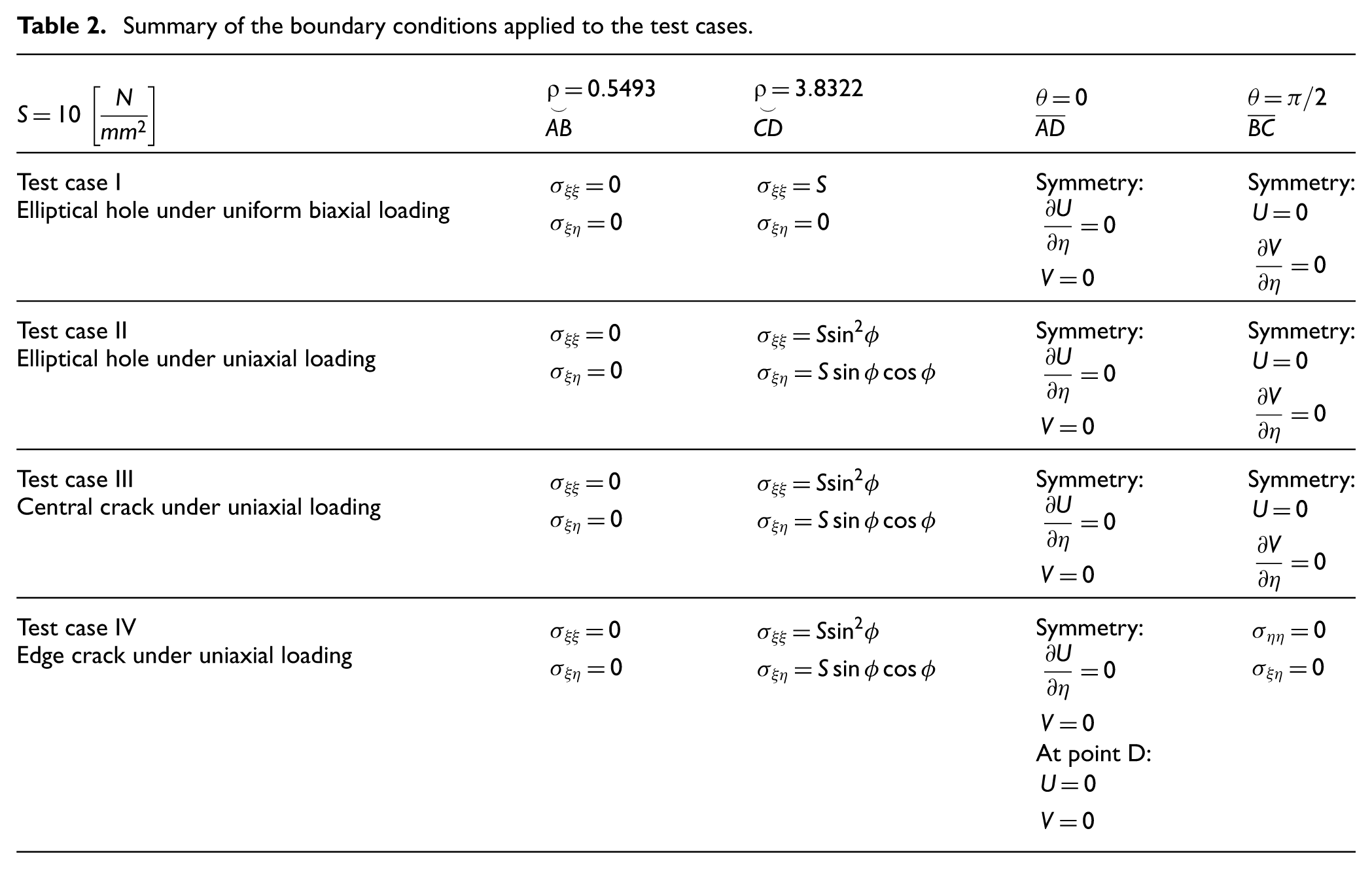
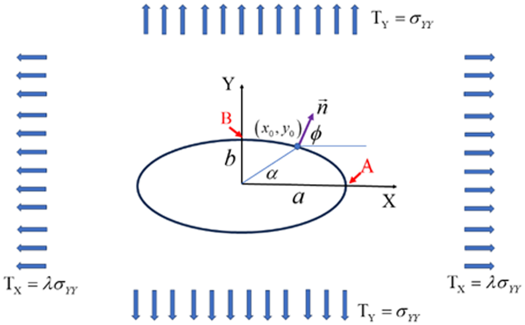
Table 2 presents the boundary conditions applied in the four test cases. In the previous usage of this FD technique,^10,11 the crack tip lay at a boundary point on which the boundary conditions were applied. In the EHCS, crack tip A is the corner point $(ξ, η) = (1, 1)$ , as shown in Figure 2(b). The two difference equations corresponding to the imaginary corner mesh point near tip A were modified to impose the boundary conditions $\frac{\partial U}{\partial η} = 0, V = 0$ on the tip. Further details are provided in Appendix 1.

Figure 4.

Elliptical hole under remote biaxial loading.

Table 2.

Summary of the boundary conditions applied to the test cases.

$S = 10 [\frac{N}{m m^{2}}]$	$ρ = 0.5493$ $\overset{⌣}{AB}$	$ρ = 3.8322$ $\overset{⌣}{CD}$	$θ = 0$ $\bar{AD}$	$θ = π / 2$ $\bar{BC}$
Test case I Elliptical hole under uniform biaxial loading	$\begin{matrix} σ_{ξ ξ} = 0 \\ σ_{ξ η} = 0 \end{matrix}$	$\begin{matrix} σ_{ξ ξ} = S \\ σ_{ξ η} = 0 \end{matrix}$	Symmetry: $\begin{matrix} \frac{\partial U}{\partial η} = 0 \\ V = 0 \end{matrix}$	Symmetry: $\begin{matrix} U = 0 \\ \frac{\partial V}{\partial η} = 0 \end{matrix}$
Test case II Elliptical hole under uniaxial loading	$\begin{matrix} σ_{ξ ξ} = 0 \\ σ_{ξ η} = 0 \end{matrix}$	$\begin{matrix} σ_{ξ ξ} = S \sin^{2} ϕ \\ σ_{ξ η} = S \sin ϕ \cos ϕ \end{matrix}$	Symmetry: $\begin{matrix} \frac{\partial U}{\partial η} = 0 \\ V = 0 \end{matrix}$	Symmetry: $\begin{matrix} U = 0 \\ \frac{\partial V}{\partial η} = 0 \end{matrix}$
Test case III Central crack under uniaxial loading	$\begin{matrix} σ_{ξ ξ} = 0 \\ σ_{ξ η} = 0 \end{matrix}$	$\begin{matrix} σ_{ξ ξ} = S \sin^{2} ϕ \\ σ_{ξ η} = S \sin ϕ \cos ϕ \end{matrix}$	Symmetry: $\begin{matrix} \frac{\partial U}{\partial η} = 0 \\ V = 0 \end{matrix}$	Symmetry: $\begin{matrix} U = 0 \\ \frac{\partial V}{\partial η} = 0 \end{matrix}$
Test case IV Edge crack under uniaxial loading	$\begin{matrix} σ_{ξ ξ} = 0 \\ σ_{ξ η} = 0 \end{matrix}$	$\begin{matrix} σ_{ξ ξ} = S \sin^{2} ϕ \\ σ_{ξ η} = S \sin ϕ \cos ϕ \end{matrix}$	Symmetry: $\begin{matrix} \frac{\partial U}{\partial η} = 0 \\ V = 0 \end{matrix}$ At point D: $\begin{matrix} U = 0 \\ V = 0 \end{matrix}$	$\begin{matrix} σ_{η η} = 0 \\ σ_{ξ η} = 0 \end{matrix}$

4.3. Results

The obtained numerical results were compared with known analytical results.

4.3.1. Case I: Infinite elastic plate with an elliptical hole subjected to remote uniform biaxial loading

Four geometries were solved: $b / a = 0.1, 0.25, 0.50, 0.75$ . Here, a = 20 mm. The numerical results for the circumferential stress along the elliptical face $\overset{⌣}{AB}$ in Figures 3(a) and 2(b) are compared with the analytical results obtained by Gao:⁵

σ_{η η} (ρ_{0}, θ) = \frac{4 S \frac{b}{a}}{(1 + \frac{b^{2}}{a^{2}}) - (1 - \frac{b^{2}}{a^{2}}) \cos (2 θ)}

(17)

At the ellipse tip (A), $θ = 0$ . Hence, Equation (15) can be reduced to:

σ_{η η} (ρ_{0}, 0) = 2 S \frac{a}{b}

(18)

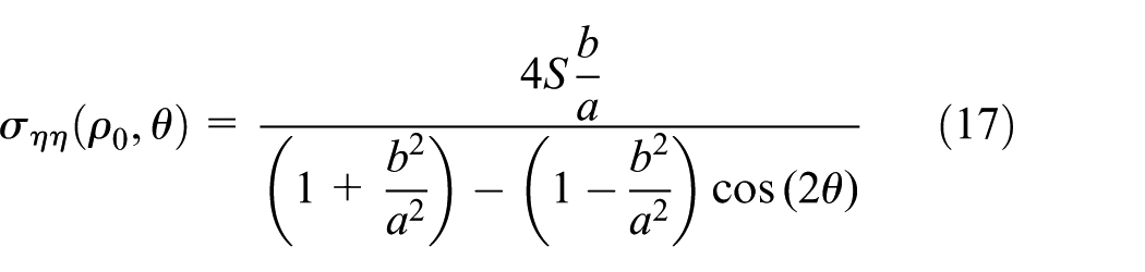
The numerical results, which is the symmetry line in Figures 2(b) and 3(a), are compared with previous analytical results⁵ in which hyperbolic function expansions, mathematical manipulations, and simplifications are applied to obtain them in a simple Cartesian coordinate form:¹⁸ $\bar{AD}$

σ_{η η} (ρ, 0) = σ_{Y Y} (X) = S \frac{X (X^{2} - a^{2} + 2 b^{2})}{{(X^{2} - a^{2} + b^{2})}^{\frac{3}{2}}} .

(19)

For X = a (at Tip A), Equation (19) is identical to Equation (18).

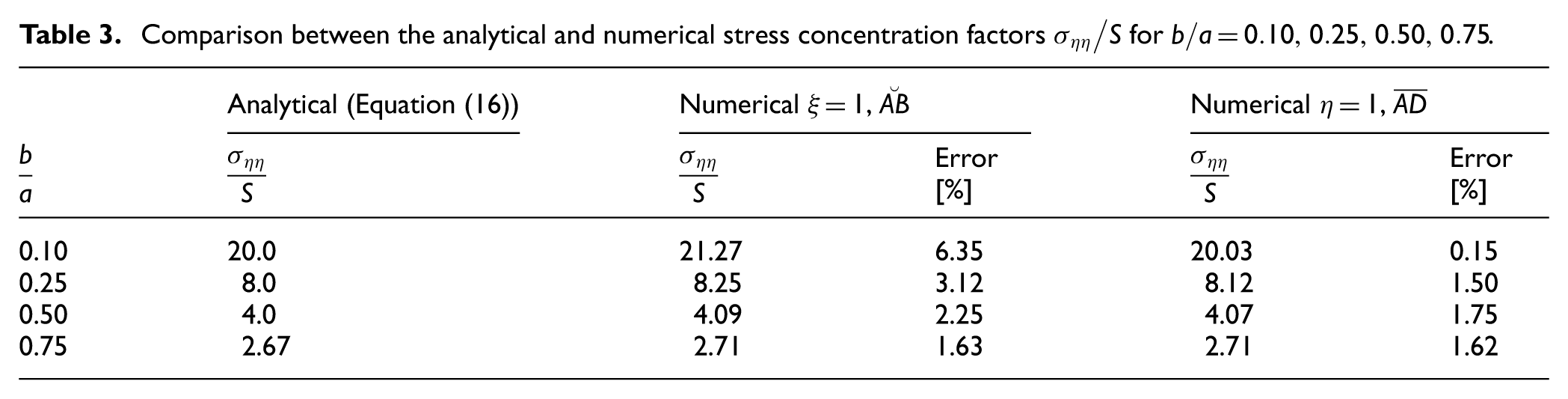
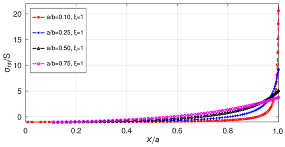
Figure 5(a) shows a comparison between the numerical and analytical results for $b / a = 0.1, 0.25, 0.50, 0.75$ along the ellipse face $\overset{⌣}{AB}$ and the symmetry line at $θ = 0$ $\bar{AD}$ . The stress $σ_{η η}$ was compared for $0 \leq X / a \leq 10$ , where $0 \leq X / a \leq 1$ corresponds to the ellipse face $\overset{⌣}{AB}$ and $1 \leq X / a \leq 10$ corresponds to the symmetry line $\bar{AD}$ . In Figure 5(a), only the region $0.8 \leq X / a \leq 1.2$ is shown, because in this region, the gradients are steep, and the four examples can be distinguished. The numerical results are plotted with lines and markers. Each marker represents the value on a boundary point. The analytical results are plotted with lines (cyan line: no markers). A very good agreement can be observed visually. The highest errors should occur for $b / a = 0.1$ , since the gradients for this case are the steepest. Figure 5(b) shows a plot of the analytical and numerical results for the region $0.98 \leq X / a \leq 1.02$ near Tip A. The analytical and numerical results show a good agreement in this region as well. Clearly, the value at the crack tip when extrapolated from the crack face $\overset{⌣}{AB}$ is slightly higher than that extrapolated from the symmetry line $\bar{AD}$ . The reason for this discrepancy is the location of Tip A. It lies at the corner (Figure 2(b)) where the boundary conditions are not uniquely defined. Tip A is at a distance of $h / 2$ from the nearest mesh point on $\bar{AD}$ and at a distance $l / 2$ from the nearest point on $\overset{⌣}{AB}$ . Two separate extrapolations are conducted using the four nearest mesh points, as shown in Figure 5(b). Table 3 presents the results. The error was calculated using the expression $(σ_{η η}^{N} - σ_{η η}^{A}) / σ_{η η}^{A} \times 100 [%]$ , where $σ_{η η}^{N}$ and $σ_{η η}^{A}$ are the numerically extrapolated and analytical exact results, respectively. Evidently, extracting the stress concentration factor from the stresses on the symmetry line leads to higher accuracy results, having a relative error lower than 1.75%. The region in which the accuracy was low was less and was confined to a normalized distance 0.3% of X/a from the tip toward the crack face ( $θ = π / 2$ ).

Figure 5.

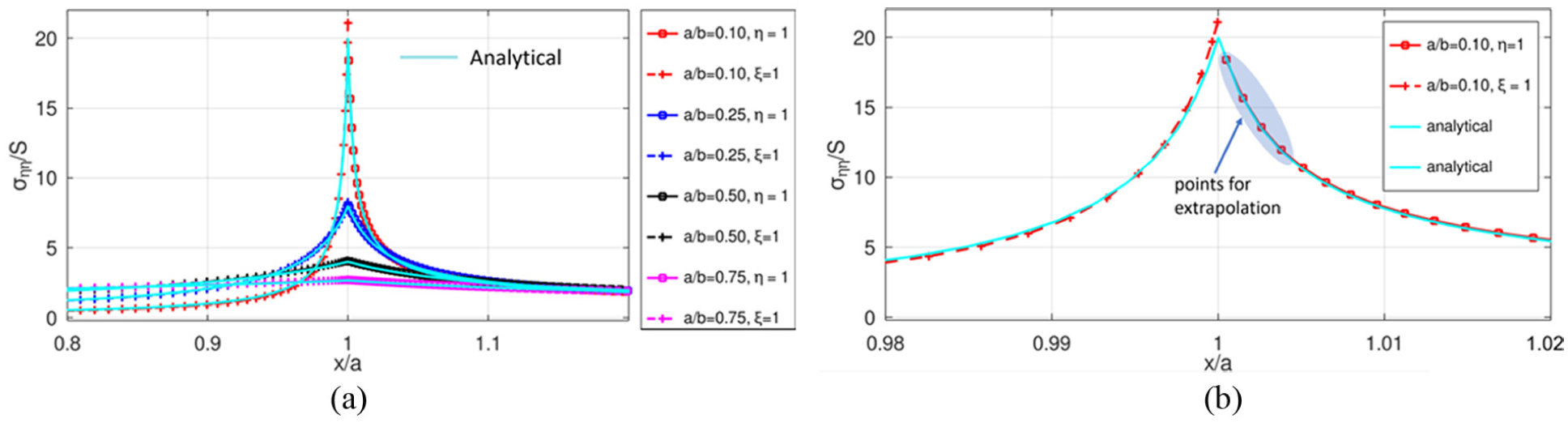
(a) Comparison between the numerical and analytical results for b/a = 0.10, 0.25, 0.50, 0.75 along the ellipse face $\overset{⌣}{AB}$ . (b) Comparison of $σ_{η η}$ with the analytical results (Equation (15)). Each marker represents a numerical result at a boundary point.

Table 3.

Comparison between the analytical and numerical stress concentration factors $σ_{η η} / S$ for $b / a = 0.10, 0.25, 0.50, 0.75$ .

	Analytical (Equation (16))	Numerical $ξ = 1$ , $\overset{⌣}{AB}$		Numerical $η = 1$ , $\bar{AD}$
$\frac{b}{a}$	$\frac{σ_{η η}}{S}$	$\frac{σ_{η η}}{S}$	Error[%]	$\frac{σ_{η η}}{S}$	Error[%]
0.10	20.0	21.27	6.35	20.03	0.15
0.25	8.0	8.25	3.12	8.12	1.50
0.50	4.0	4.09	2.25	4.07	1.75
0.75	2.67	2.71	1.63	2.71	1.62

4.3.2. Case II: Infinite elastic plate with an elliptical hole subjected to remote uniaxial loading

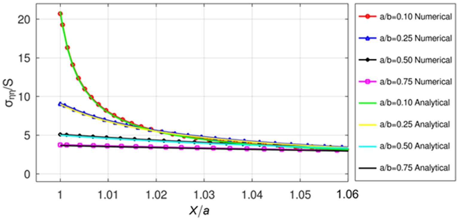
Figure 6 shows the numerical $σ_{η η} / S$ on the ellipse face at $ρ = ρ_{0}$ versus the normalized length $X / a$ for $b / a = 0.10, 0.25, 0.50, 0.75$ . With a decreasing ratio $b / a$ , the gradients near Tip A increase. The stress concentration at Tip A has been given by Inglis (1913b):

σ_{YY} = S (\frac{2 a}{b} + 1) .

(20)

The analytical solution for the stress along X > a at Y = 0 has been provided by Gao.⁵ The expression can be simplified as follows:¹⁸

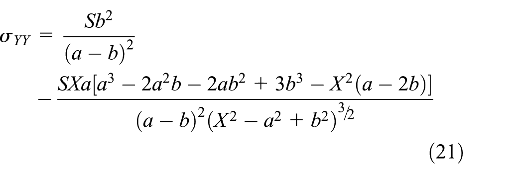
σ_{Y Y} = \frac{S b^{2}}{{(a - b)}^{2}} - \frac{S X a [a^{3} - 2 a^{2} b - 2 a b^{2} + 3 b^{3} - X^{2} (a - 2 b)]}{{(a - b)}^{2} {(X^{2} - a^{2} + b^{2})}^{\frac{3}{2}}}

(21)

The numerical results for $b / a = 0.10, 0.25, 0.50, 0.75$ are compared with the analytical results obtained using Equation (21) and shown in Figure 7(a) for the normalized region $1 \leq X / a \leq 1.06$ , where the gradients are steep. The markers represent numerical values, whereas the lines represent the analytical results obtained using Equation (19). A very good agreement was observed. The stress concentrations at Tip A (X = a) are calculated using the same extrapolation described in Section 4.3.1; Table 4 presents a summary. The accuracy was very good, and the relative error was less than 2.55% (for $η = 1$ , $\bar{AD})$ . To further verify the accuracy, the relative errors at each boundary point (not just at Tip A) were calculated. The relative error was averaged as follows:

\frac{1}{9} \int_{X / a = 1}^{X / a = 10} | error | d (X / a) .

(22)

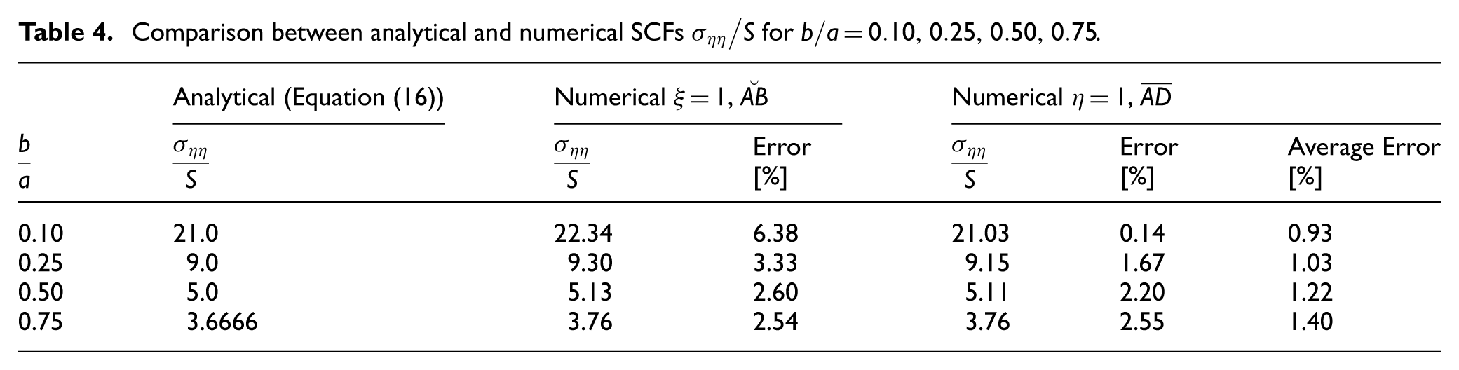
Table 4 presents the calculated values (final column). The maximum relative error at Tip A was 2.55% for $b / a = 0.75$ . The averaged maximum relative error was 1.40% for $b / a = 0.75$ .

Figure 6.

Numerical $σ_{η η} / S$ on the ellipse face at $ρ = ρ_{0}$ versus the normalized length $X / a$ for $b / a = 0.10, 0.25, 0.50, 0.75$ .

Figure 7.

Comparison of $σ_{η η} / S$ between the numerical and analytical (Equation (17)) results for Y = 0 and X > a for $b / a = 0.10, 0.25, 0.50, 0.75$ . Each marker represents a numerical result at a boundary point.

Table 4.

Comparison between analytical and numerical SCFs $σ_{η η} / S$ for $b / a = 0.10, 0.25, 0.50, 0.75$ .

	Analytical (Equation (16))	Numerical $ξ = 1$ , $\overset{⌣}{AB}$		Numerical $η = 1$ , $\bar{AD}$
$\frac{b}{a}$	$\frac{σ_{η η}}{S}$	$\frac{σ_{η η}}{S}$	Error[%]	$\frac{σ_{η η}}{S}$	Error[%]	Average Error[%]
0.10	21.0	22.34	6.38	21.03	0.14	0.93
0.25	9.0	9.30	3.33	9.15	1.67	1.03
0.50	5.0	5.13	2.60	5.11	2.20	1.22
0.75	3.6666	3.76	2.54	3.76	2.55	1.40

4.3.3. Case III: Infinite elastic plate with a central crack (2a) under remote uniaxial loading normal to the crack face

The well-known analytical solution for this problem¹⁹ can be expressed as follows:

K_{I}^{*} = S \sqrt{π a} .

(23)

The SIF was calculated from the normal stress ahead of the crack tip.

One and three terms of the asymptotic expansion were used to correlate the stress. When one term was used, the SIF was calculated according to:¹⁹

K_{I} (r_{i}) = σ_{η η} (r_{i}) \sqrt{2 π r_{i}} .

(24)

When three terms were used, the stress at r_i was approximated by:

σ_{η η} (r_{i}) = \frac{s_{0}}{\sqrt{r_{i}}} + s_{1} + s_{2} \sqrt{r_{i}} .

(25)

Here, r = X–a. Using the three values $σ_{η η} (r_{i})$ , $σ_{η η} (r_{i + 1})$ , and $σ_{η η} (r_{i + 2})$ at the three adjacent points, the coefficients $[s_{0}, s_{1}, s_{2}]$ were calculated at $r^{*} = (r_{i} + r_{i + 2}) / 2$ . The SIF was calculated as follows:

K_{I} (r^{*}) = s_{0} \sqrt{2 π} .

(26)

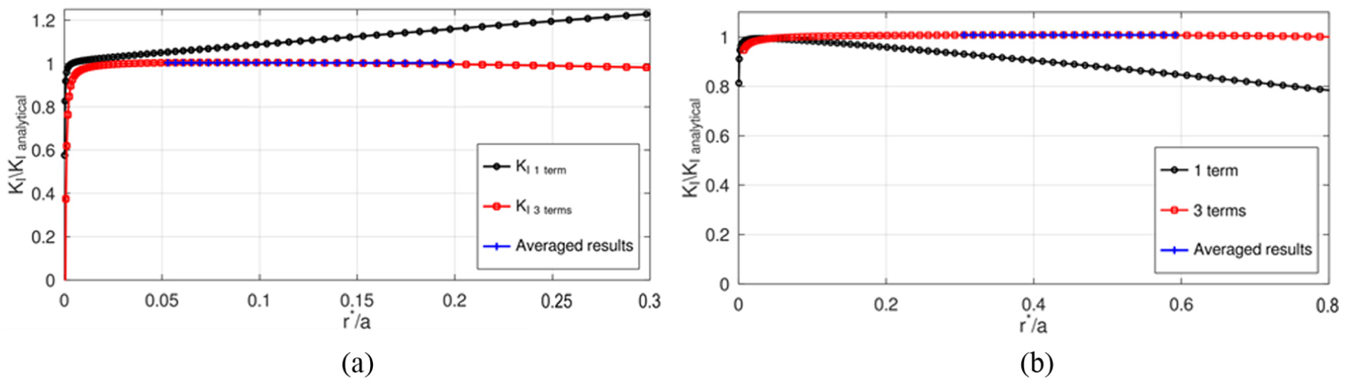
Figure 8(a) shows the results. When using only 1 term, there is no region in which the SIF is constant. The results obtained from points near the crack tip, $0 < r^{*} / a < 0.04$ , were inaccurate. The results when using three terms of the asymptotic expansion were largely identical for the region $0.05 < r^{*} / a < 0.25$ . The results for the region $0.05 < r^{*} / a < 0.20$ (blue line) were averaged to yield the value $K_{I}^{stress} / K_{I}^{*} = 1.0034$ , which represented a slight error of 0.34%.

Figure 8.

Normalized SIF calculated along $r^{*} / a$ using one and three terms of the asymptotic expansion. (a) From the normal stress ahead of the crack tip. (b) From the normal gaps behind the crack tip. The values in blue are averaged to extract the SIF.

The SIF was calculated from the normal gaps behind the crack tip using higher-order terms of the asymptotic expansion. Successful calculation of the mixed-mode SIFs using higher-order terms of the asymptotic expansion of the normal gaps and the tangential shifts behind the crack tip was performed in a previous research on interface cracks.¹¹ Owing to symmetry, only half of the normal gap was used. When one term was used in the asymptotic expansion, the SIF was calculated as:

K (r_{i}) = \frac{V (r_{i})}{\sqrt{\frac{r_{i}}{2 π}} \frac{1 + κ}{2 G}} .

(27)

Here, the shear modulus is $G = E / [2 (1 + ν)]$ , and $κ = 3 - 4 ν$ for plane strain.

The three terms of the asymptotic expansion are as follows:

V (r_{i}) = d_{0} \sqrt{r_{i}} + d_{1} {r_{i}}^{\frac{3}{2}} + d_{2} {r_{i}}^{\frac{3}{2}} .

(28)

Here, r = a − X. Using the three values $V (r_{i})$ , $V (r_{i + 1})$ , and $V (r_{i + 2})$ at three adjacent points, the coefficients $[d_{0}, d_{1}, d_{2}]$ were calculated at $r^{*} = (r_{i} + r_{i + 2}) / 2$ . The SIF can be extracted using the following expression:

K_{I} (r^{*}) = d_{0} \frac{2 G \sqrt{2 π}}{1 + κ} .

(29)

Figure 8(b) shows the results. Using only one term of the asymptotic expansion resulted in the absence of a region in which the SIF was constant. The SIF obtained using three terms from points near the crack tip, $0 < r^{*} / a < 0.05$ , was inaccurate. The results were largely identical in the region $0.05 < r^{*} / a < 0.80$ . The results in the region $0.25 < r^{*} / a < 0.60$ (blue line) were averaged to yield the value $K_{I}^{d i s p l a c e m e n t} / K_{I}^{*} = 1.0079$ , which represented an error of 0.79%. Both the results from the stresses ahead of the crack tip and from the normal gaps behind the crack tip had an error of less than 1%. This fact confirms the reliability of the FD technique presented herein.

4.3.4. Infinite elastic plate with an edge crack (a) under remote uniaxial loading normal to the crack face

The SIF results were obtained using the same methods described in Section 4.3.3, that is, higher-order terms of the asymptotic expansion for correlating the normal stress ahead of the crack tip (Figure 9(a)) and normal gaps behind the crack tip (Figure 9(b)). The normalized values obtained were 1.1876 and 1.1862 for the normal stress and normal gaps, respectively. These values were compared with the values obtained recently²⁰ using the strain energy approach and those obtained from the handbook,²¹ where w is the width of the plate.

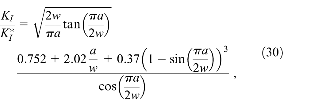
\begin{matrix} \frac{K_{I}}{K_{I}^{*}} = \sqrt{\frac{2 w}{π a} \tan (\frac{π a}{2 w})} \\ \frac{0.752 + 2.02 \frac{a}{w} + 0.37 {(1 - \sin (\frac{π a}{2 w}))}^{3}}{\cos (\frac{π a}{2 w})}, \end{matrix}

(30)

and

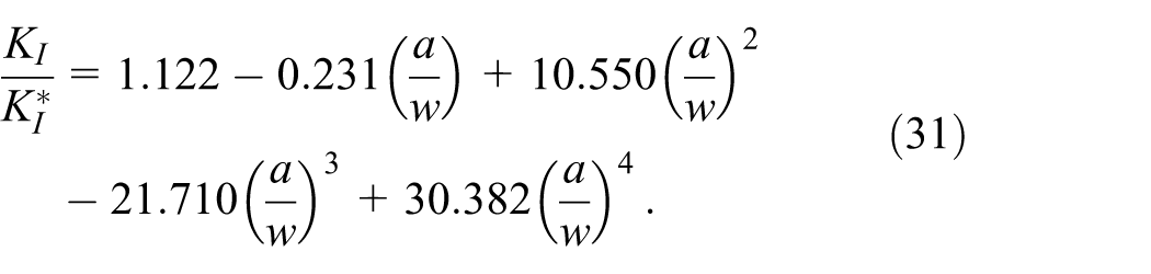
\begin{matrix} \frac{K_{I}}{K_{I}^{*}} = 1.122 - 0.231 (\frac{a}{w}) + 10.550 {(\frac{a}{w})}^{2} \\ - 21.710 {(\frac{a}{w})}^{3} + 30.382 {(\frac{a}{w})}^{4} . \end{matrix}

(31)

Table 5 presents the results.

Figure 9.

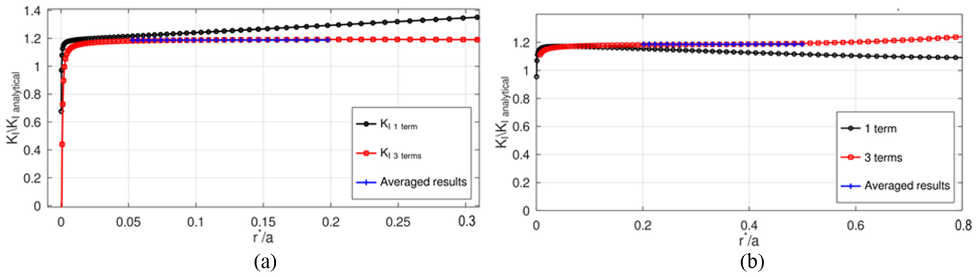
Normalized SIF along $r^{*} / a$ calculated using one and three terms of the asymptotic expansion. (a) From the normal stress ahead of the crack tip. (b) From the normal gaps behind the crack tip. The values in blue are averaged to extract the SIF.

Table 5.

Normalized K_I for edge crack.

	$\frac{K_{I}}{S \sqrt{π a}}$
$a / W$	Present workNormal stressEquations (23)–(24)	Present workNormal gapsEquations (26)–(27)	Shi and Oyadiji²⁰	Equation (30) ²¹	Equation (31) ²¹
0.1	1.188	1.186	1.191	1.196	1.186

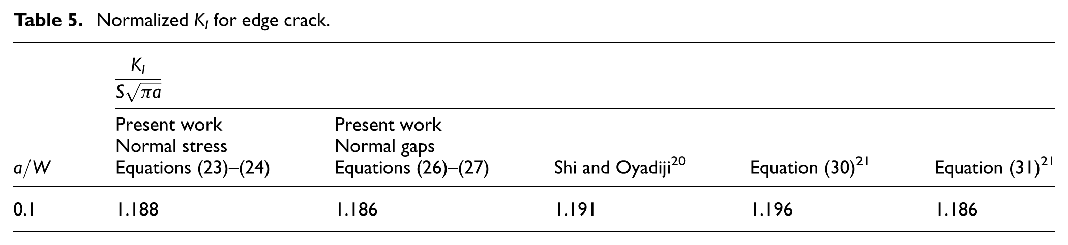
The results obtained in this study are in good agreement with previous results listed in Table 5, with a discrepancy of less than 1%. The results obtained using both methods differed by 0.17%. This confirms the reliability of the FD technique used in this study.

5. Summary and conclusions

An EHCS $(ρ, θ)$ (Equation (1)) was applied to mesh geometries with a traction-free elliptical hole subjected to uniform biaxial and uniaxial loading far from the hole. New mapping and transformation formulae (Equation (7)) were derived and applied to map the physical domain to a computational domain in which the mesh is uniform, and the axes $(ξ, η)$ align with the elliptic-hyperbolic axes. This alignment permits easy and accurate application of boundary conditions. Two-dimensional analyses were performed using an FD code, which was used earlier in several studies for Cartesian and polar transformations. This study aimed to check the capability of this technique in predicting SCFs and SIFs due to the presence of an elliptical hole. Four elliptical geometries were analyzed ( $b / a = 0.10, 0.25, 0.50, 0.75$ ) and subjected to uniform biaxial loading and unidirectional loading.

The results were compared with the analytical results, yielding a very good agreement. The maximum relative error at the tip of the ellipse in the case of uniform biaxial loading was less than 1.6%. In the case of unixial loading, it was less than 2.55%, and the average error was estimated to be less than 1.4%. For b = 0, the ellipse degenerated into a crack. Two crack problems were analyzed: a central crack and an edge crack. Both cracks were subjected to unidirectional tension. The SIFs were calculated from the normal stresses ahead of the crack tip and from the normal opening of the crack face behind the crack tip. One and three terms of the asymptotic expansion were used to correlate the stress and displacement. The relative error of the two methods was less than 1%.

The implementation of the elliptic-hyperbolic mesh, in conjunction with the proposed mapping technique, significantly enhances the capability of the FD method to accurately resolve problems involving elliptical holes and cracks. Furthermore, this approach can be extended to analyze cracks emanating from elliptical apertures, accounting for complex phenomena such as crack face contact and friction in both homogeneous and functionally graded materials (FGMs). In addition, the framework is well-suited to address interface crack problems, hydraulic fracturing, stamping, and inclusion-related studies.

Footnotes

Appendix 1

Two difference equations were applied for the corner mesh point adjacent to tip A. The two equations adopt the symmetry conditions at Tip A:

(32)

\frac{\partial U}{\partial η} = 0,

(33)

V = 0 .

The derivatives on the boundary $η = 1$ are as follows:

(34)

{\frac{\partial U}{\partial η} |}_{1} (ξ = - \frac{h}{2}) = \frac{U (1, 2) - U (1, 1)}{l},

(35)

{\frac{\partial U}{\partial η} |}_{2} (ξ = \frac{h}{2}) = \frac{U (2, 2) - U (2, 1)}{l},

(36)

{\frac{\partial U}{\partial η} |}_{3} (ξ = \frac{3 h}{2}) = \frac{U (3, 2) - U (3, 1)}{l},

(37)

{\frac{\partial U}{\partial η} |}_{4} (ξ = \frac{5 h}{2}) = \frac{U (4, 2) - U (4, 1)}{l} .

Using a third-order polynomial for $\frac{\partial U}{\partial η} (ξ)$ :

(38)

\begin{matrix} {\frac{\partial U}{\partial η} |}_{tip A} (ξ = 1) = \frac{5}{16} {\frac{\partial U}{\partial η} |}_{1} + \frac{15}{16} {\frac{\partial U}{\partial η} |}_{2} - \frac{5}{16} {\frac{\partial U}{\partial η} |}_{3} \\ + \frac{1}{16} {\frac{\partial U}{\partial η} |}_{4} = 0 \end{matrix}

Substituting Equations 34 to 37 into Equation 38 yields the following equation:

(39)

\begin{matrix} U (1, 2) - 3 U (2, 1) + 3 U (2, 2) + U (3, 1) - U (3, 2) \\ - \frac{1}{5} U (4, 1) + \frac{1}{5} U (4, 2) - U (1, 1) = 0 \end{matrix}

The condition Equation A2 is simply:

(40)

V (1, 2) + V (2, 2) + V (2, 1) + V (1, 1) = 0 .

Equations 39 and 40 were used to obtain values $[U (1, 1), V (1, 1)]$ for the corner mesh point.

Appendix 2

The solution of an infinite elastic plate with an elliptical hole which is subjected to remote uniform biaxial loading was conducted using 3 different meshes. For this case, b = 10 mm and a = 20 mm (Figure 2). The applied load was located at a distance of ∼10a. The meshes were as follows: $110 \times 46$ , $165 \times 69$ , and $220 \times 92$ . The first number corresponds to the number of mesh point in the $ρ$ direction and the second to the number of points in the $θ$ direction (Equations 1(a) and (b)). All other parameters are detailed in Sections 4 and 4.3.1.

The coefficients to be used with Equation (6) are given in Table 6.

The three meshes are shown in Figure 11.

The resulting stress $σ_{yy}$ due to the three meshes for $1 \leq \frac{X}{a} < 10$ along y = 0 is shown in Figure 12. It can be observed that all the three lines which correspond to the three different meshes coincide. This fact means that the results converge. The analytical solution for this case is $\frac{σ_{yy}}{S} = 5$ . It can also be observed that already for $\frac{X}{a} = 6$ the stress $\frac{σ_{yy}}{S}$ drops to 1 which is the applied force at infinity. In this study, the mesh of $220 \times 92$ was used to minimize the discretization error and the load was applied at $\frac{X}{a} = 10$ which is far enough from the ellipse.

Acknowledgements

The author would like to thank all those people who made the following software available on the Internet free of charge: Intel^® Fortran Compiler OneAPI 2025, the FORTRAN library Y12m on Netlib, and GNU Octave version 10.2.0, and also thank Editage () for English language editing.

ORCID iD

Avraham Dorogoy

Funding

The author received no financial support for the research, authorship, and/or publication of this article.

Declaration of conflicting interests

The author declared no potential conflicts of interest with respect to the research, authorship, and/or publication of this article.

Author biography

Avraham Dorogoy holds a BSc and MSc in Mechanical Engineering from the Technion—Israel Institute of Technology, and a PhD from Tel Aviv University, Israel. He previously served as a senior research engineer in the Dynamic Fracture Laboratory at the Technion, where he conducted numerical simulations for materials under dynamic loading, large deformations, and plasticity, while also teaching fracture mechanics as an adjunct lecturer. Currently, he is a Senior Research Engineer at Tel Aviv University and a scientific consultant for Plasan Sasa Ltd., Israel.

References

Patel

. Effect of various discontinuities present in a plate on stress concentration: a review. Eng Res Express 2022; 4: 032001. https://doi.org/10.1088/2631-8695/ac8c1b

Inglis

. Stresses in a plate due to the presence of cracks and sharp corners. Trans Inst Naval Archit 1913; 55: 219–241.

Muskhelishvili

. Some basic problems of mathematical theory of elasticity. Noordhoff, 1953.

Timoshenko

Goodier

. Theory of elasticity. 3rd ed. McGraw-Hill, 1969.

Gao

. A general solution of an infinite elastic plate with an elliptic hole under biaxial loading. Int J Press Vessels Piping 1996; 67: 95–104. https://doi.org/10.1016/0308-0161(94)00173-1

Kanezaki

Nagata

Murakami

. New closed-form solution by Cartesian coordinate for stress distribution around elliptic hole and its applications. J Math Mech Mater Phys 2007; 1: 232–243. https://doi.org/10.1299/jmmp.1.232

Yosibash

Szabó

. Convergence of stress maxima in finite element computations. Commun Numer Methods Eng 1994; 10: 683–697. https://doi.org/10.1002/cnm.1640100903

Wang

Qin

. A new special element for stress concentration analysis of a plate with elliptical holes. Acta Mech 2012; 223: 1323–1340. https://doi.org/10.1007/s00707-012-0650-z

Sun

. Explicit equations to transform from Cartesian to elliptic coordinates. Math Med Appl 2017; 2: 43. https://doi.org/10.11648/j.mma.20170204.12

10.

Dorogoy

Banks-Sills

. Shear loaded interface crack under the influence of friction: a finite difference solution. Int J Numer Methods Eng 2004; 59: 1749–1780. https://doi.org/10.1002/nme.936

11.

Dorogoy

Banks-Sills

. Effect of crack face contact and friction on Brazilian disk specimens—a finite difference solution. Eng Fract Mech 2005; 72: 2758–2773. https://doi.org/10.1016/j.engfracmech.2005.05.005

12.

Dorogoy

Banks-Sills

. A rigid punch on an elastic half-space under the effect of friction: a finite difference solution. In: Seiniger

Winner

Gail

(eds) Automotive systems; bioengineering and biomedical technology; computational mechanics; controls; dynamical systems, Vol 2. ASMEDC, 2008, pp.259–271. https://doi.org/10.1115/ESDA2008-59159

13.

Dorogoy

. Finite difference method for solving crack problems in a functionally graded material. Simulation 2019; 95: 941–953. https://doi.org/10.1177/0037549718802894

14.

Dorogoy

. Shear–compression loaded interface crack between a rigid substrate and an FGM layer—frictional crack closure effects. Int J Fract 2019; 216: 149–159. https://doi.org/10.1007/s10704-019-00348-y

15.

Zlatev

Wasniewski

Schaumburg

. Y12M, solution of large and sparse systems of linear algebraic equations: documentation of subroutines. Springer-Verlag, 1981. https://doi.org/10.1007/3-540-10874-2

16.

Eaton

Bateman

Hauberg

, et al. GNU octave version 10.2.0 manual: a high-level interactive language for numerical computations, https://docs.octave.org/latest/ (2025, accessed 25 June 2026).

17.

Intel Corporation. Intel® Fortran Compiler, Intel® oneAPI HPC Toolkit. Version 2025. Santa Clara (CA): Intel Corporation, https://www.intel.com/content/www/us/en/developer/tools/oneapi/fortran-compiler-download.html (2025, accessed 25 June 2026).

18.

Oore

. Explicit solutions in Cartesian coordinates for an elliptic hole in an infinite elastic plate. Math Mech Solids 2025; 30: 765–791. https://doi.org/10.1177/10812865241249751

19.

Anderson

. Fracture mechanics: fundamentals and applications. 4th ed. Taylor & Francis Group, 2017. https://doi.org/10.1201/9781315370293

20.

Shi

Oyadiji

. Mixed mode stress intensity factors of single edge cracked/notched plates under different boundary conditions using strain energy approach. Fatigue Fract Eng Mater Struct 2023; 46: 2229–2243. https://doi.org/10.1111/ffe.13994

21.

Tada

Paris

Irwin

. The stress analysis of cracks handbook. 3rd ed. ASME Press, 2000. https://doi.org/10.1115/1.801535