Social Class Origin and Assortative Mating in Britain,1949

Abstract

This article examines trends in assortative mating in Britain over the last 60 years. Assortative mating is the tendency for like to form a conjugal partnership with like. Our focus is on the association between the social class origins of the partners. The propensity towards assortative mating is taken as an index of the openness of society which we regard as a macro level aspect of social inequality. There is some evidence that the propensity for partners to come from similar class backgrounds declined during the 1960s. Thereafter, there was a period of 40 years of remarkable stability during which the propensity towards assortative mating fluctuated trendlessly within quite narrow limits. This picture of stability over time in social openness parallels the well-established facts about intergenerational social class mobility in Britain.

Keywords

assortative mating homogamy inequality marriage social stratification

Introduction

In this article our aim is to describe the pattern of assortative mating (AM) – the tendency for like to marry or cohabit with like – as it has evolved over six decades in Great Britain. The tendency for birds of a feather to flock together is well known. Our particular focus is on the social class origins of conjugal partners. Social class origins as a concept can be interpreted in a number of ways but in this study, primarily for reasons of data availability, we concentrate on the social class of the fathers of married and cohabiting couples.

Those that study marriage patterns make a distinction between AM and homogamy. A homogamous marriage pattern is one where there is a tendency for people with a particular characteristic to marry individuals with the same characteristic. Thus, to use the example of religious confession, Catholics are more likely to marry other Catholics than adherents of another confession. However, Catholics that do not marry Catholics tend to marry within the broad Christian Trinitarian tradition rather than choose a partner who is a Muslim or Jewish. When partner choice is non-random with respect to an attribute we speak of assortative mating, thus homogamy is a special case of AM. Turning to social class background, there is a well-known tendency for people to marry partners with the same class background as their own and, if they do not, to choose partners from classes that are in close social and economic proximity to their own. Both types of choice contribute to the commonly observed association between the social class backgrounds of conjugal partners.

It is possible to examine AM from a number of perspectives and for a number of reasons. Our interest is in AM as an indicator of the openness of the structure of social stratification. The degree of AM in a society is the outcome of a complex mixture of social processes reflecting both choice and constraint. Partners are chosen from among the set of potential mates known to the chooser. Some factors operate to constrain the content of this ‘risk set’ – for example, geography and factors correlated with it, like the degree of socio-economic segregation, will have a powerful effect. Other factors influence the choice made among the set of possible partners. Some of these will reflect the choosers’ notions of social similarity and social acceptability. Both types of factors are relevant to the genesis of the degree of openness of a society’s social stratification regime. In a caste like society homogamy would be the rule and people would only marry partners with a similar class background. In a completely open society the social class background of partners would be statistically independent. Any actually existing society will lie between these two extremes and this position may change in a systematic way over time.

Examining trends in who marries whom complements studies of intergenerational social class mobility. One of the motivations for studying intergenerational social mobility is the belief that it reveals something about the openness of a society. If social class origins are strongly related to social class destination then rates of social mobility will be low and we may speak of a relatively closed social stratification regime. If social class origins are only weakly related to social class destinations then rates of social mobility will be high and we have a relatively open social stratification regime.

Low levels of social mobility are usually interpreted as indicating inequalities in life-chances. Another way of putting this is to say that low social mobility societies are less integrated. Low levels of intermarriage between the social classes can be interpreted in a similar way (patterns of intermarriage between ethnic groups are often regarded as indicators of ethnic integration). Of course the mechanisms that produce a given rate of social class mobility will not be exactly the same as those that produce a given rate of class based AM. However, there are likely to be many common factors and it is of obvious interest to establish whether both sources of evidence point to similar or divergent conclusions about progress towards a more open, more integrated society.

The complementarity of evidence about intergenerational and marital mobility has not gone unnoticed. Towards the end of a review of Goldthorpe (1980), Runciman (1980: 159) remarks that:

The implications of the […] findings [about social mobility] for the questions about class formation and social structure cannot be elucidated without relating them to the very topics that this volume does not attempt to deal with, such as patterns of marriage.

And goes on to say: ‘[b]ut mobility ratios […] are only one of the sources on which a diagnosis of the changing class structure of twentieth century Britain must rest’. We take his comments to be well founded and in this article we make a modest effort to fill the ellipsis.

Context and Question

The study of who marries whom is closely related to the study of social mobility and indeed was a part of the first major British empirical investigation of the latter (Glass, 1954). Since then, at least in Britain, interest has predominantly focused on intergenerational social class mobility to the neglect of marriage. Insofar as attention has been paid to the association between the characteristics of marital partners, this has mostly focused, in Britain and elsewhere, on the similarity between their education (Blossfeld and Timm, 2003; Halpin and Chan, 2003; Kalmijn, 1991b, 1994; Katrňák et al., 2006; Mare, 1991; Smits, 2003; Ultee and Luijkx, 1990), religious confession (Kalmijn, 1991a), ethnicity (Muttarak and Heath, 2010), geographical distance (Coleman, 1984) and parental wealth (Charles et al., 2013).

Undoubtedly the reason that there have been more studies of assortative mating by educational level than by any other characteristic is the availability of data. However, there is one seldom mentioned drawback to focusing on education – its endogeneity. The process of finding a marriage partner and obtaining an education can have reciprocal effects on each other. In the past a woman might curtail her education once she found a suitable partner. Given typical differences between the sexes in age at marriage we would then observe a certain amount of hypergamy – a tendency for women to ‘marry up’ in educational terms – that is actually somewhat spurious. The apparent hypergamy might mask the fact that people of similar latent educational ability, or indeed similar social origins, marry each other despite the fact that their achieved educational qualifications differ. As average age at marriage increases and various forms of consensual union that are not perceived to be incompatible with remaining in education become more common, the proportion of couples with the same level of education may appear to increase, while in a sense what has changed are social mores about gender roles and educational participation, not the intrinsic degree of marital selectivity.

We do not dismiss the study of AM in terms of the educational characteristics of the partners – it is certainly of interest in its own right – but for our purpose, which is the study of long term trends, choosing a criterion of similarity which is exogenous with regard to the process being studied is advantageous. The indicator being measured is not the outcome of choices made by the subjects under investigation. They have a degree of choice about the type and length of their education but they can’t choose their parents.

Turning to British studies that directly deal with AM specifically in terms of class origins, the earliest modern contribution is Berent’s chapter in Glass (1954) which concludes, on the basis of the simple statistical techniques available at the time, that AM by social class background declined during the first half of the 20th century. But though there are some notable contributions on other countries (Girard, 1964; Kalmijn, 1991b; Mäenpää, 2015; Mäenpää and Jalovaara, 2015; Uunk et al., 1996) few have built on Berent’s foundations and examined whether in Britain the tendency for people to choose marriage partners from similar class backgrounds as themselves has increased, decreased or remained essentially unaltered. Both Miles (1999) and Penn (1984) use English and Welsh marriage register data to examine change in patterns of marital choices, but while both of these studies are of interest they are of limited use for our purposes. Miles’ study is based on a small collection of parishes and in any case is mostly concerned with the late 19th century, while Penn’s is concerned with marriages taking place within one urban area in the north-west of England. Neither provides a secure basis for extending Berent’s pioneering work into the early 21st century.

If intermarriage between social groups, such as social classes, is a function of the economic and social distance between them then the level of AM can also be thought of as an indicator of the openness of the class structure. Viewed in this way – as providing a macro level index of openness at a particular point in time – patterns of AM, even as revealed by data on the stock of marriages and partnerships, which is the only sort of data we have in abundance – can be revealing.

Imagine that we have data on the social class origins of married couples. We define a set of mutually exclusive class categories and form a square contingency table that cross-classifies husbands and wives by their social class origins. A set of such tables for different time points will be the main focus of our interest. The probability that someone from a given social class background will marry someone with a similar background can be thought of as a function of two things: the proportion of potential partners with that background (i.e. the marginal distribution of social class) and the propensity to choose similar rather than different partners (the association between class backgrounds) given the distribution of potential partners. It is this propensity that is principally of interest to us and which we interpret as an index of societal openness.

Naturally our interest is in long term changes or trends, but what should these look like? We are not interested in mere differences, we would not expect the degree of openness in contiguous years to be exactly the same. Of more interest is evidence of persistent and enduring trends that either tend to increase or reduce openness. Of course, there is no reason to expect a constant trend in one direction over the entire period we consider – that would be too restrictive – but we will be reluctant to talk of anything but trendless fluctuation unless we see clear evidence of a persistence of trend direction over several independent contiguous data-points.

What should we expect to find? This is far from clear. An influential hypothesis advanced by Smits et al. (1998) in a cross-national study of the educational similarity of spouses is that the strength of educational homogamy follows an inverted U shape trajectory. Homogamy first decreases and then increases driven by various social and economic processes subsumed under the labels of modernization, industrialization and economic development. This hypothesis is of doubtful relevance to a study of post-war Britain: modernization and industrialization having long been achieved and it has been empirically rejected by Halpin and Chan (2003). They find that since the 1970s educational homogamy has actually declined which they interpret as a consequence of the lengthening of the gap between the termination of full-time education and first marriage. Whether we should expect to find a similar sort of pattern with respect to AM by social class origin is a moot point.

Another source of expectations is the social mobility literature, but here we face the embarrassment of conflicting evidence. Scholars investigating trends in social mobility from a social class perspective unanimously agree that in the past 40 years British relative mobility rates have not trended in any particular direction and therefore that the degree of openness of the social stratification regime is best characterized as trendless fluctuation (Goldthorpe and Mills, 2008). On the other hand, economists studying social mobility from the point of view of income mobility conclude that the relative mobility rates of a cohort born in 1970 are significantly lower than those of a cohort born in 1958 (Blanden et al., 2004). This has been widely interpreted in the popular press, think-tanks and government circles as signifying that Britain has a ‘mobility problem’ and has become a less open society.

It is clear to us that there are no strong grounds either theoretical or empirical for forming a clear set of expectations about what we might observe and that therefore the best course of action is to simply see what the empirical evidence reveals.

Data

We use social survey data from Great Britain on the contemporaneous stock of ‘marital’ unions in which both partners are 25–59 years of age.¹ Where possible we distinguish between England and Wales (E&W) and Scotland. The data sources are listed in Appendix Table A1.² Data of sufficient comparability and quality for this age-range are available for 13 different years between 1949 and 2009/2010. No distinction is made between marital and consensual unions as the latter are not distinguished in the oldest data-sets. We have examined the importance of the distinction in the later data and found no detectable difference in AM between marital and non-marital unions with respect to social class origin.

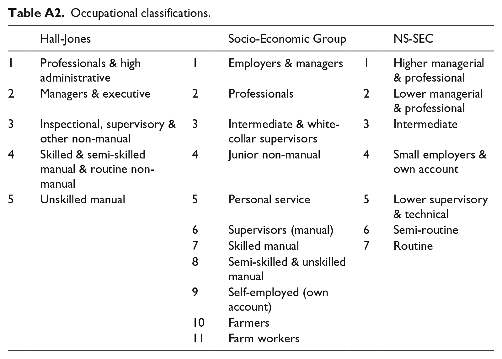
The basic unit of analysis is a husband’s father’s occupation (HFO) by wife’s father’s occupation (WFO) cross-classification. We have 25 such tables. We are not able to categorize occupations in the same way in all periods. In 1949, 1959/1960 and 1972 the data are coded into five Hall Jones (HJ) categories (Hall and Jones, 1950; Moser and Hall, 1954). From 1972 through to 1993 we use 11 aggregated Socio-Economic Groups (SEG) and from 1991 to 2009/2010 seven National Statistics Socioeconomic Classification (NS-SEC) categories. Category labels are given in Appendix Table A2.³ Our primary aim is to work with as disaggregated a set of categories as the data will sustain.

Because we use different categorizations we cannot directly compare the level of AM across the three periods. However, we are able to splice the three series together by double coding the occupational information in the 1972 Oxford Social Mobility (OSM) survey data (HJ/SEG) and in the 1991 British Household Panel Survey (SEG/NS-SEC). This means that there is an overlap between the end point of the first period – 1972 – and the start of the second period and likewise between the end of the second period and the start of the third. We can make inferences about trends within periods and, more tentatively, between periods if within period trends move in the same direction.

Statistical Models

If parental occupations were represented by a continuous socio-economic status scale an obvious way to proceed would be to calculate correlation coefficients and examine how they change over time. This, however, is ruled out by the nature of the occupational coding adopted in many of the data-sets. In the majority all we have is a limited number of categories, most commonly an abbreviated version of Office for National Statistics’ (ONS) Socio-Economic Group. Though some sort of ordering could be imposed on the categories, it is not clear in practice how best to go about it. Faute de mieux our strategy is to treat the occupational categories as categorical and make no assumptions about their ordering. This leads us naturally to use log-linear and closely related models (Bishop et al., 1975) to make smoothed representations of the main features of the pattern of association in HFO by WFO contingency tables and of how this changes over time.

An important point of reference is the model of common association:

L o g (F_{i j k}) = λ + λ_{i k} + λ_{j k} + λ_{i j}

(1)

where Log(F_ijk) is the natural logarithm of the estimated expected frequency in row i (HFO), column j (WFO), layer k (survey), for i = 1 to I and j = 1 to J occupational groups and k = 1 to K surveys. The λ_ik, λ_jk and λ_ij terms are sets of association parameters to be estimated and the un-subscripted λ is a constant. The model is hierarchical and to avoid clutter we adopt the convention of writing it in terms of association and interaction parameters leaving out lower level parameters. Our main interest is in the λ_ij estimates for these tell us about the pattern and intensity of AM.

An implication of model 1 is that the log-odds ratios that describe the HFO by WFO association are identical in each layer and thus correspond to the hypothesis of common association across surveys.

Equation 2 represents a simple way of quantifying differences in the HFO by WFO association over survey years that is commonly termed the log-multiplicative layer effect model (Erikson and Goldthorpe, 1992; Xie, 1992):

L o g (F_{i j k}) = λ + λ_{i k} + λ_{j k} + ϕ_{k} ψ_{i j}

(2)

In this model we allow a common pattern of HFO by WFO association (ψ_ij) to vary across survey years with the difference across survey years estimated by K-1 log-multiplicative parameters (φ_k). The model is identified by restricting φ₁ = 1, thus values of less than 1 imply a weakening of association in the layer concerned compared to the level in the baseline category (all log-odds ratios shrink towards zero by a constant proportion).

The φ_k parameters from equation 2 tell us much of what we want to know about change over time. However, we also want to form an idea of what it is that is changing. The common association model estimates (I-1)(J-1) association parameters. Clearly as the size of the tables examined grows the problem of comprehending the association structure becomes acute. The smallest tables we examine are 5 by 5, the largest 11 by 11. Even the small tables give us 16 unique odds ratios from which all the others can be derived. It greatly aids comprehension if we can visualize the implied structure of association.

An attractive way to do this is to use the RC(M) association model (Clogg and Shihadeh, 1994). This structures the HFO by WFO association in terms of estimated scores for the I rows (u_i) and J columns (v_j) and a set of M association parameters φ_m. If M = 1, φ₁ directly estimates the log-odds ratio for rows i and i" and columns j and j" when the score difference in both rows and columns is equal to 1. The model is flexible in the sense that u_i and v_j are not constrained to follow the order of the rows and columns in the I by J table. Thus we can discover empirically the ordering of the categories and the distances between them. A generalization of the model is to allow M to be greater than 1. This partitions the row by column association into the sum of multiplicative components. In the case of a three-way IJK table:

L o g (F_{i j k}) = λ + λ_{i k} + λ_{j k} + \sum_{m = 1}^{M} ϕ_{m} u_{i m} v_{j m}

(3)

A number of simplifications and extensions of the RC(M) association model are useful. In all our models, we restrict the scores for father’s social class to be the same whether they refer to the husband’s father’s or the wife’s father’s class; that is, I = J and u_{1m =} v_1m, u_2m = v_2m…, u_Im = v_Jm for m = 1 to M. This facilitates the construction of easy to interpret bi-plots.

Equation 3 specifies a model that assumes the HFO by WHO association is constant across the K surveys. Simple extensions of the RC(M) model involve allowing the intrinsic association parameters to vary by survey (replacing φ_m with φ_mk) giving us a partially heterogeneous model. Allowing both the φ_m as well as the u_im and v_jm scores to vary by survey gives us a fully heterogeneous model.

All the models reported in this article were estimated using either Lem (Vermunt, 1997) or the R package gnm (Turner and Firth, 2007).

Results

We present our results separately for three time periods 1949–1972, 1972–1993 and 1991–2009/2010.

1949–1972

For this period we have three tables giving us time points 10 and 12 years apart. Table 1 reports the fit statistics for a number of models. The model of common association (M1) clearly does not fit the data.

Table 1.

Fit statistics for various models of 5 x 5 x 3 cross-classifications of husband’s father’s occupation by wife’s father’s occupation by survey, 1949, 1959/1960, 1972. N = 9021.

Model	Description	L²	d.f.	p	Δ	BIC
M1	Common association	111.9	32	.00	3.0	−179.5
M2	M1 + log-multiplicative layer effect	44.0	30	.05	1.7	−229.3
M3	RC(1)	169.5	44	.00	3.7	−231.2
M4	RC(1) partially heterogeneous	104.8	42	.00	3.4	−277.7
M5	RC(1) fully heterogeneous	95.6	36	.00	3.0	−236.3
M6	RC(2)	129.7	41	.00	3.2	−244.2
M7	RC(2) partially heterogeneous	54.2	36	.03	2.1	−273.6
M8	RC(2) fully heterogeneous	36.6	27	.10	1.6	−209.3
M9	M7 with homogeneous ϕ for m=2	63.2	38	.01	2.2	−282.9

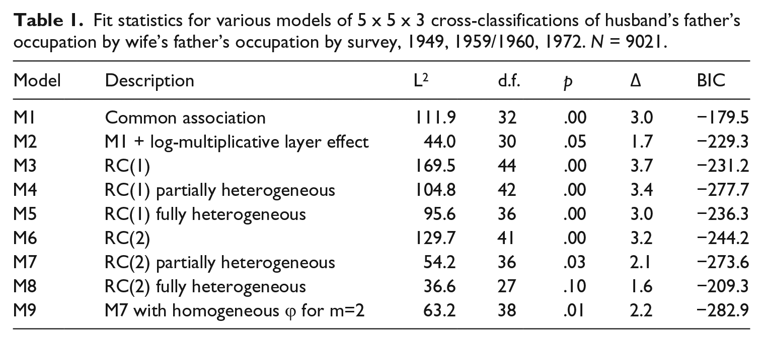
M2 estimates log-multiplicative parameters that index the relative strength of a uniform proportional change in all the log-odds ratios. It fits the data (just) by the standard convention. The φ_k are 1, 1.07, 0.61. In other words the propensity towards AM appears to have weakened between 1959/1960 and 1972.

But what is the structure of association that has weakened? A simple way to answer this question is to find a RC(M) model that gives an adequate representation of the data and then make a plot of the row and column scores with the axes defined by the M dimensions. Models M3 through M9 give a record of the search.

An adequate representation of the data requires two dimensions (M = 2), the first of which is by far the most important. To represent the structure of change over time we need only allow the intrinsic association parameter for the first dimension (φ_1k) to vary over the K (survey year) tables.⁴ Model M9 provides the estimated scores which for the 1949 survey are plotted in Figure 1 in the adjusted form x_i= u_1i √ φ_1k and y_i= u_2i √ φ_2k.

Figure 1.

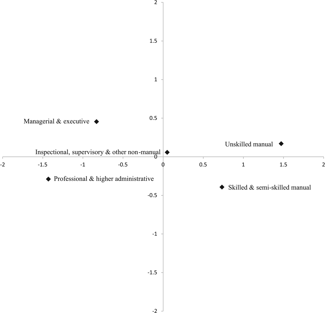
Bi-plot of adjusted category scores from RC(2) model M9 (Table 1). Only the scores for 1949 are plotted.

Pairs of points that are close together represent pairs of occupations that are closer to independence than pairs that are further apart. How should we understand this? One way is to say that they exchange sons and daughters roughly in proportion to their sizes. Another is to say that such occupations are similar in their propensity (net of the absolute size of the categories concerned) to exchange sons and daughters with occupations that are more distant. The complete configuration of points can be interpreted as representing the social and economic distances between occupations and these distances give a visual representation of the pattern and strength of social openness. The effect of the differing intrinsic association parameters for the first dimension is, in the case of 1959/1960, to move all the coordinates slightly away from the origin in the direction of the x axis and for 1972 to shrink all points towards the origin.⁵ When all points shrink towards the origin a decrease in overall association is implied, that is, an increase in openness.

What then of the apparent change that took place during the decade of the 1960s? One possibility is that the decline in association between 1959/1960 and 1972 is the result of measurement error. To make the three surveys in the 1949–1972 period comparable, the cross-classification of the Office of Population Census and Survey (OPCS) 1970 occupational unit groups (OUGs) and employment statuses has been coded into the categories of the Hall-Jones scale.⁶ It is well known that there is no standardized way to do this and in fact some commentators have been sceptical about the possibility of reproducing the Hall-Jones scale at all (Hope, 1981, 1984; Macdonald, 1974, Townsend, 1979). What is clear is that we cannot know for sure whether we have coded the 1972 data appropriately. Purely random coding errors would have the effect of attenuating the HFO by WFO association and thus could account for what we observe.

But there is another possibility. Perhaps at least part of the change is real. After all the period in question is the 1960s. Would it be so peculiar if people became less constrained in their choice of marriage partners at a time when so many other social constraints were being rejected by those of marriageable age? This suggests that we should look more closely at the data taking into account year of marriage and the average age of the couple in the year they were surveyed. Thus in 1972 we distinguish between those who married in 1961–1972 and those married before that and between those who in 1972 were aged 25–37 and those aged 37.5–59. We make the same kind of distinctions for the 1949 and 1959/1960 surveys – marriage year in the former divided at 1939 and in the latter at 1950. Thus in each survey we have four groups: (1) the relatively old with long marriage durations; (2) the relatively young (who married young) with long marriage durations; (3) the relatively old with short marriage durations (presumably late marriages and remarriages); (4) the relatively young who married relatively recently. It is the behaviour of this last group that we are most interested in.

There are insufficient observations in group 3 in the 1959/1960 data so these are dropped giving us a total of K = 11 tables. We estimated log-multiplicative layer effect models for the 11 sub-tables and tested a number of restrictions to the multiplier coefficients. The best model requires only three φ_k parameters: one that applies to all the 1949 and 1959/1960 sub-tables, one that applies to groups 1 to 3 in 1972 and one for group 4 in 1972. The third parameter is smaller than the other two suggesting a weaker pattern of AM among young and recently married people in 1972. In other words the generally weaker association (greater openness) in 1972 was partly driven by the recent marriages of the young, which is what an explanation in terms of the generalized effects of cultural change in the 1960s would predict.

Though far from definitive the evidence is strong enough to at least raise the possibility that what we observe is not simply an artefact of a particular set of occupational coding decisions. Perhaps, at least for a brief period during which cultural if not economic change was particularly rapid, the propensity for like to marry like in Britain was indeed somewhat reduced.

1972–1993

For this period we have 19 tables, clustered within two sub-periods, 1972–1976 and 1989–1993. In addition we distinguish between England and Wales (11 tables) and Scotland (eight tables). We start with our conclusion: we can find no convincing evidence of any sustained trend towards greater or lesser openness. Admittedly, we must qualify this by saying that we have no observations for the 12 years from 1977 to 1988, but whatever happened during that time, the propensity of like to marry like was at roughly the same level at the beginning of the 1990s as it had been at the beginning of the 1970s.

Considering all 19 tables simultaneously (Table 2) we should remember that the large sample size (N = 50,795) allows us to detect trivial differences between tables and will make it almost impossible to find any simple model that fits the data at conventional significance levels. The common association model M1 does not fit the data though it only misclassifies 5 per cent of the cases.

Table 2.

Fit statistics for various models of 11 x 11 x 19 cross-classifications of husband’s father’s occupation by wife’s father’s occupation by survey, 1972–1993. N = 50,795.

Model	Description	L²	d.f.	p	Δ	BIC
M1	Common association	1,938.2	1,800	.01	5.2	−17,565.8
M2	M1 + log-multiplicative layer effect	1,840.4	1,782	.02	5.2	−17,402.5
M3	RC(1) + diag	2,495.6	1,879	.00	5.7	−17,864.5
M4	RC(1) + diag partially heterogeneous	2,458.1	1,861	.00	5.6	−17,706.8
M5	RC(2) + diag	2,017.7	1,870	.01	5.4	−18,244.8
M6	M5 with homogenous ϕ for m=2	1,980.8	1,851	.02	5.3	−18,075.8

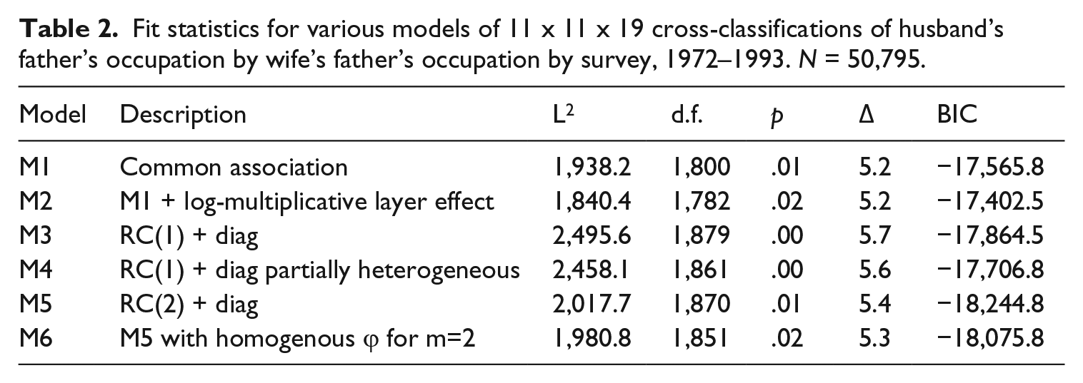
Adding log-multiplicative terms (M2) improves model fit and inspection of the standardized residuals reveals no obvious pattern that is informative either about structure or change.

Figure 2 shows a plot of the log-multiplicative parameters and their quasi-confidence intervals (Firth, 2003) for M2. The figure reveals several interesting patterns. First, the HFO by WFO association appears generally higher in Scotland than it is in E&W. The amount of overlap of the confidence intervals should, however, caution against exaggerating the national difference. Second, there is little evidence of change in AM propensities when we compare the 1970s with the late 1980s and early 1990s. Point estimates wobble up and down and confidence intervals overlap considerably.

Figure 2.

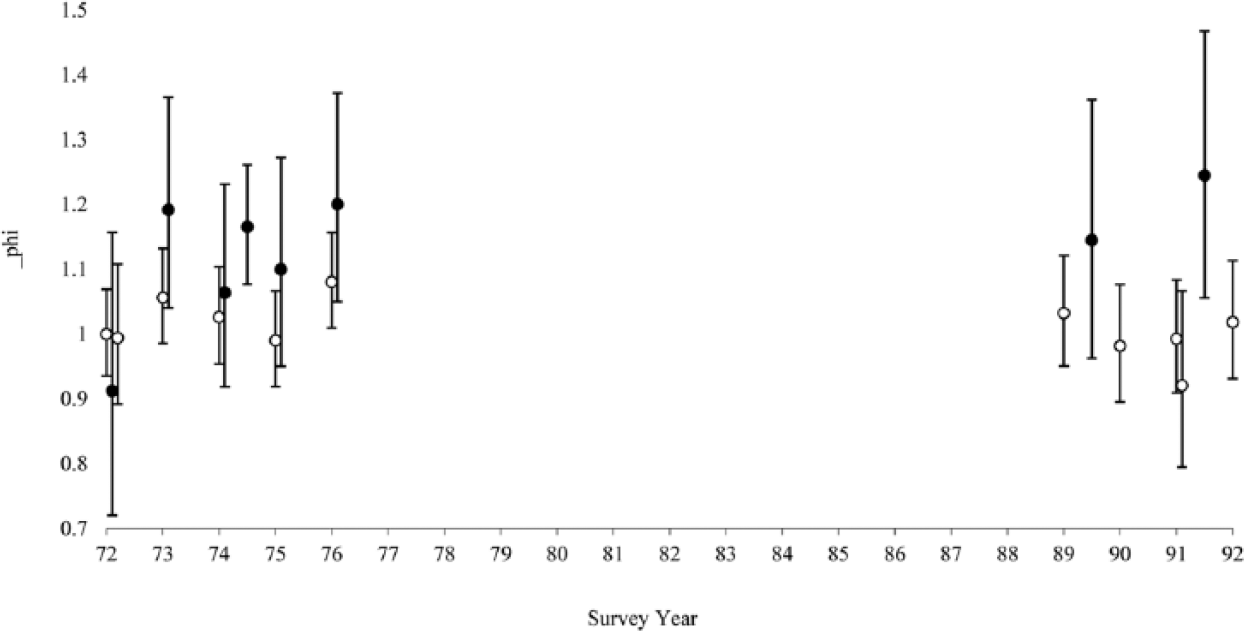
Log-multiplicative parameter estimates and 95 per cent quasi confidence intervals plotted by survey year, 1972–1993. Model M2 (Table 2). E&W (clear) Scotland (solid), couples aged 25–59.

To represent the pattern of association we return to the RC(M) model. It turns out that in this case it is necessary to partition HFO by WFO association in a slightly different way. As well as estimating row and column scores we also need to estimate parameters for the main diagonal of the HFO by WFO margin. In other words we cannot capture association involving cells on the main diagonal in terms of the u_mi = v_mj scale scores alone and in fact all log-odds ratios for these cells are a function of the intrinsic association parameters, the scale scores and the relevant parameters for the main diagonal.

The fit statistics for Models M3–M6 in Table 2 are a record of our search for a parsimonious RC(M) model. Model 6 which assumes two dimensions of association and heterogeneous intrinsic association with respect to the first dimension seems to give a smoothing of the data that is adequate for our purposes. The 19 intrinsic association parameters for the first dimension reproduce closely the pattern revealed by the log-multiplicative parameters plotted in Figure 2 – slightly greater association in Scotland than in E&W and little overall difference in level of association between the earlier and later clusters.

Figure 3 is produced from pooled data. Data are pooled separately for Scotland and E&W and then a distinction is made between two periods: 1972–1976 and 1989–1993. Model M6 is then estimated for the four tables. The figure plots the coordinates for E&W 1989–1993, but we would obtain an indistinguishable pattern if we had chosen any one of the other three possibilities. Figure 3 is rather easy to interpret. If we were to rotate the axes 45° anti-clockwise towards the north-west we would find one axis that appears to represent a socio-economic status dimension with the sons and daughters of the professionals at one end and the children of manual and personal service workers at the other. The second dimension distinguishes the agricultural occupations from the rest, indicating a geographical, as much as an economic and social constraint on the choice of a marriage partner.

Figure 3.

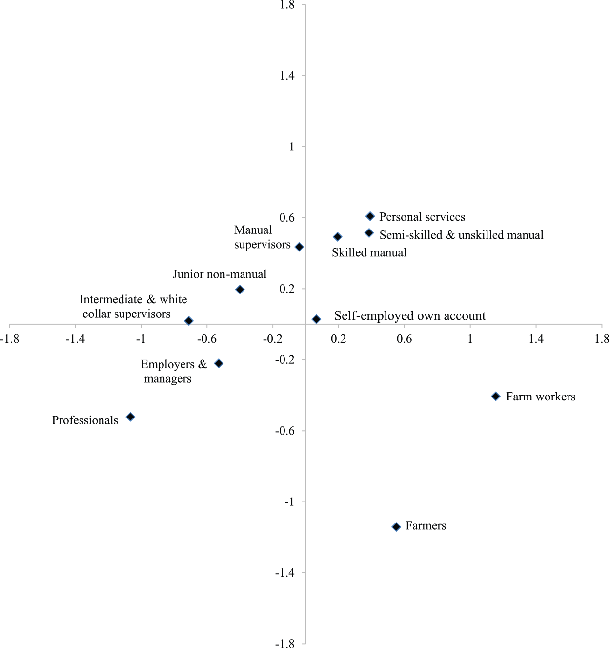
Bi-plot of adjusted category scores from RC(2) model for pooled England and Wales 1989–1993. Model 6 (Table 2).

1991–2009/2010

For this period we have three surveys but a gap of 14 years between the first and the second. Table 3 reports the fit statistics for a large number of models between which there is little to choose. The common association model (M1) does not fit at conventional levels, though it misclassifies less than 4 per cent of cases. Allowing the HFO by WFO association to vary over the three surveys (M2) does not improve the fit to the data.

Table 3.

Fit statistics for various models of 7 x 7 x 3 cross-classifications of husband’s father’s occupation by wife’s father’s occupation by survey, 1991–2009/2010. N = 10,375.

Model	Description	L²	d.f.	p	Δ	BIC
M1	Common association	104.8	72	.01	3.5	−561.0
M2	M1 + Log-multiplicative layer effect	104.2	70	.01	3.5	−543.1
M3	RC(1) + diag	123.2	95	.03	3.9	−755.3
M4	M6 partially heterogeneous	123.1	93	.02	3.9	−736.9
M5	M6 fully heterogeneous	112.4	83	.02	3.7	−655.1
M6	RC(2) + diag	119.9	90	.02	3.9	−712.3
M7	M6 with homogenous ϕ for m=2	116.2	87	.02	3.7	−688.3
M8	M6 partially heterogeneous	109.4	85	.04	3.7	−676.6
M9	M6 fully heterogeneous (m=1) Partially heterogeneous (m=2)	94.2	75	.06	3.2	−598.9
M10	M6 fully heterogeneous (m=2) Partially heterogeneous (m=1)	92.2	75	.09	3.2	−601.4
M11	M6 fully heterogeneous	88.0	68	.05	3.1	−540.7

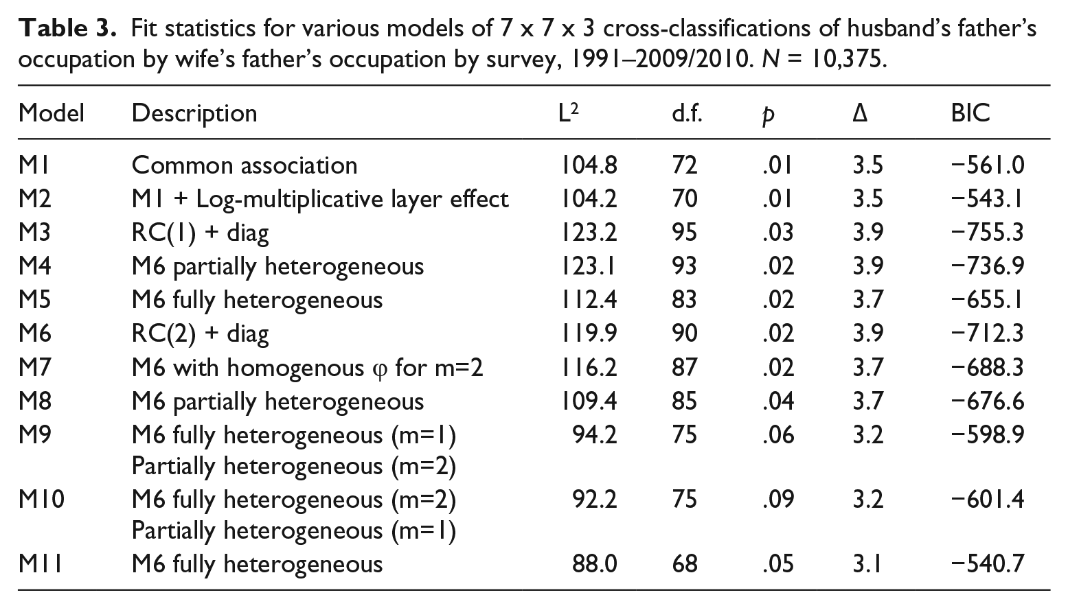
A cautious observer would insist that a model of no change that does not fit by conventional criteria and a log-multiplicative model that does not significantly improve matters cannot demonstrate the absence of substantively important change. It is entirely possible that change might not be captured by assuming that all log-odds ratios are multiplied by a constant.

To focus on this possibility let us consider model M10 which does fit the data by conventional standards. This is an RC(2) model that assumes a set of main diagonal parameters that are constant over all three tables, row/column scale scores and intrinsic association parameters relating to the second dimension that vary over tables and first dimension intrinsic association parameters (but not scale parameters) that vary over tables. This representation clearly allows over time differences that are not constrained to be proportional.

Figure 4 is a bi-plot of the estimated occupational scale scores from model M10 for the three survey years. Most striking is the impression of trendless fluctuation. At the top and the bottom of the first (horizontal) dimension each occupation’s points are rather tightly packed together and show no particular tendency over time to move either towards the origin (which would indicate a weakening of association) or away from it.

Figure 4.

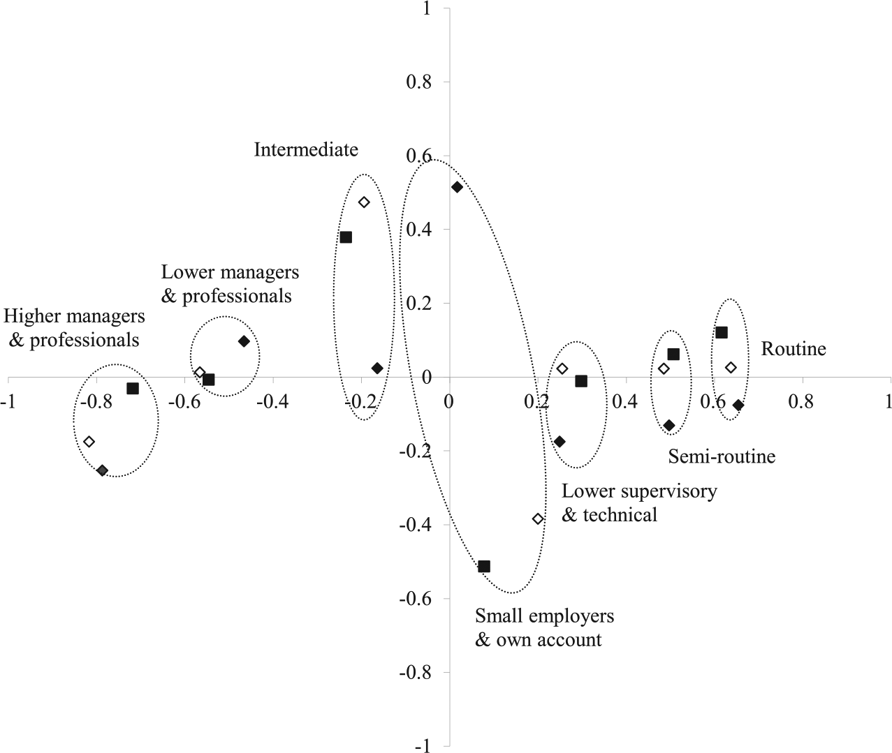
Bi-plot of adjusted category scores from RC(2) model M10 (Table 3) for Great Britain 1991, 2005, 2009/2010. 1991 clear diamond, 2005 solid diamond, 2009/2010 solid square.

But what of change along the second (vertical) dimension? Our interpretation of this is informed by the observation that these data are almost as well represented in one dimension as in two. Note that model 3, which assumes one dimension with constant occupational scale scores and constant intrinsic association, fits reasonably well and actually has the lowest Bayesian information criterion (BIC) score. Further evidence of the fragility of the second dimension comes from an inspection of the relevant occupational clusters in Figure 4. It would appear that the differences captured by this dimension largely relate to a difference between 2005 and the other two survey years with respect to the intermediate occupations and the small employers/own account workers. It is implausible to believe that such differences between data collected in 2005 and 2009/2010 can be anything other than measurement error, perhaps exaggerated by the fact that both occupational categories are rather small.⁷ Whatever the reason for these apparent differences, they have little bearing on the main fact that emerges from the plot: there is little evidence to support the idea of a generalized systematic change in the propensity towards AM.

Discussion

We began this article with a simple descriptive aim. In the body of the article we set out the somewhat involved chain of inferences we make from a large body of data. The evidence impels us towards the conclusion that between 1949 and 1959/1960 the propensity towards AM by parental class origin was stable. Between 1959/1960 and 1972 there may have been a decline in this propensity. The evidence is not conclusive but we cannot exclude the possibility that during the 1960s conjugal partner choices became less constrained by social class origins which implies that this aspect of the British stratification system became more open and consequently society more socially integrated. However, during the rest of our six decade observational window the predominant pattern is one of stability or trendless fluctuation. In particular there is no convincing evidence of systematic change between 1972 and 2010 towards greater openness.

Before commenting on the wider significance of these findings we answer an obvious objection to these conclusions. It could be claimed that by analysing the stock of marriages at a sequence of time points we have adopted a strategy that is particularly likely to favour finding continuity rather than change. In any two consecutive survey years most of the population, though aged by one year, is drawn from the same birth cohorts. In two consecutive years the magnitude of the change in AM that would be required to detect a difference would be enormous.

However, consider the period for which we have the largest quantity of evidence – 1972–1993. In 1993 more than 60 per cent of the birth cohorts present in 1972 are no longer observed, yet the pattern and level of AM in 1993 is similar to that observed in 1972. If our mode of analysis is blinding us to change then the pace of change must be so glacial that we have little hope of detecting it with social survey evidence.

One of the points of this article is to demonstrate the utility of reinstating the study of social class based AM as part of the study of social stratification. What is most striking about our results is that they parallel rather closely what we know about trends in openness in Britain from the study of intergenerational social class mobility. In that field the standard finding is that there are no trends (Bukodi et al., 2015; Goldthorpe and Mills, 2008). Class based inequalities, as indexed by relative mobility rates, fluctuate without obvious direction. Our findings on AM reinforce this picture of a social stratification regime that is remarkably stable. It also leads us to the view that the currently fashionable and widely accepted belief that Britain has an acute ‘social mobility problem’ (Social Mobility Commission, 2016) is tenable only under a highly partial and selective account of the evidence. It is of course possible to maintain that British society is not as open and socially integrated as it should be but our evidence cannot be taken to indicate that over the post-war period things have got worse.

In some ways our results are actually surprising. The social demography of British society has changed quite markedly in the last 60 years. Average age at first marriage first fell and then rose; marriage dissolution rates increased as did rates of premarital and post-divorce cohabitation; marriage markets expanded as larger proportions of a birth cohort entered the melting pot of higher education; the gender composition of higher education changed markedly; female rates of full-time labour market participation expanded; the earnings gap between men and women decreased. All of these could conceivably have had an effect on the degree of AM observed in the stock of conjugal households. But as far as we can tell, in the main, they did not or they had effects in various directions which cancelled each other out. More change is on the horizon, most significantly the rise of online dating which has the potential both to reduce the level of AM – the risk set of potential partners is massively expanded – but also to increase it – it is easier to find matches on multiple criteria of similarity.

The remaining puzzle raised by our findings, if we accept that change did occur for marriages taking place in the 1960s, is why, for a brief period, the bonds of constraint were loosened? It is tempting to point to the general relaxing of cultural norms that defined the era driven precisely by members of the birth cohorts who, while challenging the prevailing assumptions of a stuffy establishment, were also choosing their life-partners. By comparison becoming intergenerationally class mobile, even in times of cultural change, is likely to be hard because it is not just a matter of will: someone has to offer you a job. Marrying someone from a different class background (conditional on meeting them and gaining their agreement) is just a matter of breaking a social convention. Of course breaking conventions is never entirely easy, but it is made easier if it becomes common knowledge that others are also doing it.

Finally we would be negligent if we did not qualify our findings in one important way. Our results apply to very broad social class groupings. Undoubtedly there is heterogeneity within class groups at all levels of the occupational hierarchy. As Weber (1968: 932) observed: ‘in the so-called pure modern democracy, that is one devoid of any expressly ordered status privileges for individuals, it may be that only the families coming under the same tax class dance with one another.’ Though their parents may be found in the same categories of our class schemas it is probably true that the sons and daughters of High Court judges, minor aristocrats and investment bankers did not move in the same social circles – and hence marriage markets – as the progeny of provincial local government officers, secondary school teachers and clergymen. These are distinctions that our data cannot speak to. However, our results do portray the bigger picture of opportunity and constraint within which such finer grained choices were made and that is a start.

Footnotes

Appendix

Table A2.

Occupational classifications.

	Hall-Jones		Socio-Economic Group		NS-SEC
1	Professionals & high administrative	1	Employers & managers	1	Higher managerial & professional
2	Managers & executive	2	Professionals	2	Lower managerial & professional
3	Inspectional, supervisory & other non-manual	3	Intermediate & white-collar supervisors	3	Intermediate
4	Skilled & semi-skilled manual & routine non-manual	4	Junior non-manual	4	Small employers & own account
5	Unskilled manual	5	Personal service	5	Lower supervisory & technical
		6	Supervisors (manual)	6	Semi-routine
		7	Skilled manual	7	Routine
		8	Semi-skilled & unskilled manual
		9	Self-employed (own account)
		10	Farmers
		11	Farm workers

Acknowledgements

We wish to acknowledge the helpful comments of three anonymous referees. Richard Breen, John Goldthorpe, Hans-Peter Blossfeld have also helped us improve successive drafts as have seminar participants at the universities of Bamberg, Essex, Oxford and Sussex.

Funding

This research received no specific grant from any funding agency in the public, commercial or not-for-profit sectors.

Notes

Ursula Henz is an associate professor in the Department of Sociology, London School of Economics.

Colin Mills is an associate professor in the Department of Sociology, University of Oxford and a Professorial Fellow of Nuffield College.

References

Berent

(1954) Social mobility and marriage. In: Glass

(ed.) Social Mobility in Britain. London: Routledge.

Bishop

YMM

Fienberg

Holland

(1975) Discrete Multivariate Analysis: Theory and Practice. Cambridge: MIT Press.

Blanden

Goodman

Gregg

et al (2004) Changes in intergenerational mobility in Britain. In: Corak

(ed.) Generational Income Inequality. Cambridge: Cambridge University Press.

Blossfeld

H-P

Timm

(2003) Who Marries Whom? Educational Systems as Marriage Markets in Modern Societies. Dordrecht: Kluwer.

Bukodi

Goldthorpe

Waller

et al (2015) The mobility problem in Britain: New findings from the analysis of birth cohort data. British Journal of Sociology 66(1): 93–117.

Charles

Hurst

Killewald

(2013) Marital sorting and parental wealth. Demography 50: 51–70.

Clogg

Shihadeh

(1994) Statistical Analysis for Ordinal Variables. Los Angeles, CA: SAGE.

Coleman

(1984) Marital choice and geographical mobility. In: Boyce

(ed.) Migration and Mobility: Biosocial Aspects of Human Movement. London: Taylor & Francis.

Erikson

Goldthorpe

(1992) The Constant Flux. Oxford: Clarendon.

10.

Firth

(2003) Overcoming the reference category problem in the presentation of statistical models. Sociological Methodology 33(1): 1–18.

11.

Girard

(1964) Le Choix du Conjoint. Paris: PUF.

12.

Glass

(ed.) (1954) Social Mobility in Britain. London: Routledge.

13.

Goldthorpe

(1980) Social Mobility and Class Structure in Modern Britain. Oxford: Clarendon.

14.

Goldthorpe

Mills

(2008) Trends in international class mobility in modern Britain: Evidence from national surveys. National Institute Economic Review 205: 83–100.

15.

Hall

Jones

(1950) Social grading of occupations. British Journal of Sociology 1: 31–55.

16.

Halpin

Chan

(2003) Educational homogamy in Ireland and Britain: Trends and patterns. British Journal of Sociology 54(4): 473–495.

17.

Hope

(1981) Trends in the openness of British society in the present century. Research in Social Stratification and Mobility 1: 127–169.

18.

Hope

(1984) Intergenerational and career mobility in Britain: An integrated analysis. Social Science Research 13(1): 20–37.

19.

Kalmijn

(1991a) Trends in religious and educational homogamy. American Sociological Review 56: 786–800.

20.

Kalmijn

(1991b) Status homogamy in the United States. American Journal of Sociology 97: 496–523.

21.

Kalmijn

(1994) Assortative mating by cultural and economic occupational status. American Journal of Sociology 100: 422–452.

22.

Katrňák

Kreidl

Fónadová

(2006) Trends in educational assortative mating in Central Europe: The Czech Republic, Slovakia, Poland, and Hungary, 1988–2000. European Sociological Review 22(3): 309–322.

23.

Macdonald

(1974) The Hall-Jones Scale. In: Ridge

(ed.) Mobility in Britain Reconsidered. Oxford: Oxford University Press.

24.

Mare

(1991) Five decades of educational assortative mating. American Sociological Review 56: 15–32.

25.

Mäenpää

(2015) Homogamy in educational level and parental social class in Finland: A log-linear analysis. European Sociological Review 31(3): 253–267.

26.

Mäenpää

Jalovaara

(2015) Achievement replacing ascription? Changes in homogamy in education and social class origin. Advances in Life Course Research 26: 76–88.

27.

Miles

(1999) Social Mobility in Nineteenth and Early Twentieth-Century England. Basingstoke: Macmillan.

28.

Moser

Hall

(1954) The social grading of occupations. In: Glass

(ed.) Social Mobility in Britain. London: Routledge.

29.

Muttarak

Heath

(2010) Who intermarries in Britain? Explaining ethnic diversity in intermarriage patterns. British Journal of Sociology 61(2): 275–305.

30.

Payne

(1987) Employment and Opportunity. London: Macmillan.

31.

Penn

(1984) Skilled Workers in the Class Structure. Cambridge: Cambridge University Press.

32.

Rowntree

Pierce

(1961) Birth control in Britain. Population Studies 15(1): 3–31.

33.

Runciman

(1980) A measure of equality. Times Literary Supplement, 15 February (4012), 159.

34.

Smits

(2003) Social closure among the higher educated: Trends in educational homogamy in 55 countries. Social Science Research 32: 251–277.

35.

Smits

Ultee

Lammers

(1998) Educational homogamy in 65 countries: An explanation of differences in openness using country-level explanatory variables. American Sociological Review 63: 264–285.

36.

Social Mobility Commission (2016) State of the Nation 2016: Social Mobility in Great Britain. London: HMSO.

37.

Townsend

(1979) Poverty in the United Kingdom: A Survey of Household Resources and Standards of Living. Harmondsworth: Penguin.

38.

Turner

Firth

(2007) Generalized nonlinear models. R Statistical Computing and Graphics Newsletter 18(1): 11–16.

39.

Ultee

Luijkx

(1990) Educational heterogamy and father-to-son occupational mobility in 23 industrial nations: General societal openness or compensatory strategies of reproduction. European Sociological Review 6(2): 125–149.

40.

Uunk

WJG

Ganzeboom

Róbert

(1996) Bivariate and multivariate scaled association models: An application to homogamy of social origin and education in Hungary between 1930 and 1979. Quality and Quantity 30: 323–343.

41.

Vermunt

(1997) LEM 1.0: A general program for the analysis of categorical data. Tilburg: Tilburg University.

42.

Weber

(1968) Economy and Society (vol. 2). Berkeley, CA: University of California Press.

43.

Xie

(1992) The log-multiplicative layer effect model for comparing mobility tables. American Sociological Review 57: 380–395.

Social Class Origin and Assortative Mating in Britain,1949–2010

Abstract

Keywords

Introduction

Context and Question

Data

Statistical Models

Results

1949–1972

1972–1993

1991–2009/2010

Discussion

Footnotes

Appendix

Acknowledgements

Funding

Notes

References