
Abstract
Do schools reduce or perpetuate inequality by race and family income? Most studies conclude that schools play only a small role in explaining socioeconomic and racial disparities in educational outcomes, but they usually draw this conclusion based solely on test scores. We reconsider this finding using longitudinal data on test scores and four-year college attendance among high school students in Massachusetts and Texas. We show that unexplained differences between high schools are larger for college attendance than for test scores. These differences are arguably caused by differences between the schools themselves. Furthermore, while these apparent differences in high school effectiveness increase income disparities in college attendance, they reduce racial disparities. Social scientists concerned with schools’ role in transmitting inequality across generations should reconsider the assumption that schools either increase or reduce all disparities and should direct attention to explaining why high schools’ effects on specific outcomes and groups of students appear to vary so much.
Since the 1960s, sociologists have tried to identify schools’ effects on student outcomes (Coleman et al. 1966; Jencks et al. 1972; Raudenbush and Willms 1995). Early school effects studies were motivated by “the question of how well schools reduce the inequity of birth” (Coleman et al. 1966:36). These studies almost always estimate schools’ effects on test scores and largely conclude that variation in school quality explains a fairly small fraction of the variation in students’ test performance.
Although early studies of school effects suggest that differences in school quality do not play a large role in the transmission of disadvantage from one generation to the next, these studies may have looked for such effects in the wrong places. Improving students’ reading and math skills is a central goal of schooling, and scores on reading and math tests have nontrivial effects on adults’ economic success (Bowles, Gintis, and Osborne 2001; Johnson and Neal 1998; Olneck 1979). Nonetheless, raising test scores is not the only goal of schooling, and test scores are not the only outcome of schooling that predicts subsequent economic success.
We revisit the conventional wisdom about school effects for two main reasons. First, while few sociologists have ever believed that test scores are the only outcomes of schooling that influence children’s life chances, few have investigated how variation in school quality affects outcomes other than test scores. We cannot—or at least we should not—draw general conclusions about whether differences between public schools exacerbate or attenuate the effects of family background on children’s life chances without considering a broader range of outcomes. Recently available administrative data allow us to take significant steps in this direction, because we can now measure many longer-term outcomes for all students who attended a given school, rather than just the comparatively small samples from each school included in the most widely used National Center for Education Statistics surveys.
Second, U.S. society has changed in profound ways since the data analyzed in many studies of school effects were collected. In particular, the relative significance of race and class for children’s life chances appears to have changed substantially (Reardon 2011). Despite these changes, we still know little about the extent to which low-income children attend schools that are systematically worse at promoting some outcomes than others or whether school outcomes other than test performance are now more strongly related to parental income than to race.
In this paper, we measure schools’ effects on student outcomes using a unique longitudinal data set that includes approximately 550,000 students in Massachusetts and Texas who entered the 9th grade of a public high school in 2003 and 2004, making it one of the largest studies in the past 40 years of how differences among public high schools appear to affect students. 1 We estimate each high school’s impact on students’ 10th-grade math and reading scores and students’ probability of enrolling in a four-year college, net of 8th-grade achievement scores and other student characteristics at the end of 7th and 8th grade. We use these estimates to measure the extent to which high schools perpetuate or interrupt the intergenerational transmission of inequality.
We are not the first to use college enrollment as a measure of high school effectiveness, but we are among the first to argue that studying a broader range of school outcomes may change the conclusions we draw about the relationship between schools and inequality. This seems likely because although test scores and college enrollment are positively correlated, test scores are largely stable whereas college enrollment is relatively malleable. Acquiring reading and math skills almost always takes a long period of time. Students who cannot read or do basic arithmetic at the end of 8th grade hardly ever perform well on 10th-grade reading or math tests, no matter what they do in the interval. Attending a four-year college, in contrast, depends to a great extent on conscious choices that can be made during high school. Students who say they want to go to college at the end of 8th grade can change their minds and not go; and students who said they did not want to go to college can also change their minds and find a college that will accept them.
As a result, 8th-grade test scores are a very strong predictor of 10th-grade test scores. No 8th-grade measure, including test scores, predicts what students will do after they finish high school as well as their 7th and 8th-grade test scores predict their 12th-grade scores. This is not just a technical problem. It is inherent in the nature of the two outcomes. Students can change their college plans in the blink of an eye. Family background certainly influences these choices, but as we shall see, standard socioeconomic status (SES) measures do not greatly improve our ability to predict college attendance once we account for 8th-grade test scores and whether students were eligible for federally subsidized lunches. Other important non–test score outcomes that we do not consider here—such as high school graduation, arrests, and earnings—mostly fall between these extremes of stability and malleability.
Likewise, we are not the first to draw attention to how schools’ effects on racial and socioeconomic inequality vary across these outcomes and across schools. This article takes one empirical step in that direction by augmenting reading and math scores with four-year college attendance data. In the long run, however, studies of school effects should include a much broader array of outcomes that affect the adult well-being of individual students and society as a whole. These outcomes include such things as whether students complete high school, get arrested, get steady jobs, vote, have children they are too young to support, and eventually earn enough to support themselves and their children.
The Intergenerational Transmission Of Inequality
Schools play a central role in sociological accounts of how inequality is transmitted from parents to children. Two main views dominate this literature. Social and cultural reproduction theorists argue that schools perpetuate or exacerbate disparities in family background, because children from more privileged families attend better schools and have better experiences within any given school than do less privileged children (Bourdieu and Passeron 1977; Bowles and Gintis 1976; Lareau 2003). A second set of scholars argues that schools serve a compensatory function, acting as a “great equalizer” that reduces initial inequalities between social classes (Alexander, Entwisle, and Olsen 2001; Downey, von Hippel, and Broh 2004). The different views of the “reproductionists” and the “equalizers” derive, in part, from relying on different counterfactuals (in addition to different methodological approaches). The reproductionists compare the status quo to what they think would happen if all children attended identical schools and had identical experiences in them. The equalizers compare the status quo to what they think would happen if there were no schools. Recent work on elementary grades blends these two traditions, arguing that elementary schools reduce class differences but increase black-white differences in test scores (Condron 2009; Downey et al. 2004).
Despite their differences, reproductionist and equalizing perspectives tend to treat school quality as one-dimensional, assuming that enrolling disadvantaged children in good (effective) schools will attenuate inequalities based on both social class and race, whereas bad (ineffective) schools will reproduce or widen such inequalities. However, the validity of these assumptions may depend on the outcome.
A large literature documents the impact of traits not captured by test scores on educational attainment and labor market success (Farkas 2003; Heckman and Rubenstein 2001; Olneck 1979). These traits are often called noncognitive skills, although this label is somewhat misleading: All these skills involve cognition, and some are character traits, habits, dispositions, and aspirations rather than skills. They include such things as cognitive and emotional self-regulation, self-discipline, task persistence, and executive function (Duckworth and Seligman 2005; Duncan et al. 2007). Schools that successfully cultivate such attributes may or may not be equally good at raising test scores, but they may nonetheless help students stay out of serious trouble, complete high school, complete college, and earn a living.
A few studies also examine high schools’ effects on outcomes other than test scores. Jencks and Brown (1975) found that high schools’ effects on test scores, educational attainment, and occupational status are weakly correlated with one another. Using the National Educational Longitudinal Study (NELS) of 1988, Rumberger and Palardy (2005) found that high schools effective at improving test scores are not necessarily effective at reducing transfer or dropout rates. More recently, Altonji and Mansfield (2011) estimate that attending a high school at the 10th versus the 90th percentile of the school quality distribution increases the predicted probability of high school graduation and four-year college enrollment by about 10 and 20 percentage points, respectively.
Some of the most persuasive evidence on this relationship takes advantage of random assignment by studying oversubscribed high schools that use lotteries to select some of their applicants. Deming (2011) and Deming and colleagues (2012) found that disadvantaged students in the Charlotte-Mecklenburg school district who won a lottery to attend their first-choice high school were less likely to be arrested and more likely to attend a four-year college, but they found no evidence that lottery winners’ test scores rose more than the scores of students who lost the same lottery. Booker and colleagues’ (2009) study of charter schools in Florida and Chicago and Cullen, Jacob, and Levitt’s (2006) study of Chicago high schools also found that gains on outcomes other than test scores were not always accompanied by test score gains. Although these results draw largely on urban districts, where variation in school quality may be greatest, they still suggest that a theory of school effectiveness based solely on test scores will likely miss other potentially important dimensions of school quality that influence the transmission of social and economic advantages from parents to children.
Schools can have different effects on different outcomes for at least three reasons. First, some outcomes may be easier to influence than others. An hour spent on the Pythagorean theorem may have less impact than an hour spent explaining how federal financial aid works. It may also be easier to persuade 11th graders that they should apply to a four-year college than to improve their reading or math skills. Second, improving particular outcomes may require resources that are unequally distributed across schools. If a high school’s success in getting students to attend college depends to a significant extent on whether it has a guidance counselor who gets students to fill out college applications or who uploads their high school transcripts, high schools with such a counselor will outperform otherwise similar high schools in sending graduates to college, even if the high school is no better than average at teaching reading and math. Third, schools may prioritize different goals because of an explicit school policy, pressure from parents or the state, or other idiosyncratic reasons. Even when schools have the same goals, external pressures may force them to prioritize different outcomes. For example, schools facing sanctions for low test scores may prioritize raising scores even if doing so reduces the percentage of students who come to school on any given day. To the extent that students of different racial or socioeconomic backgrounds attend schools that prioritize different outcomes, schools’ effects on racial and socioeconomic inequality may vary by outcome.
Do High School Effects Vary by Student Group?
A second implicit assumption embedded in much of the early work on school effects is that school quality has the same impact on all students attending a school. The Coleman Report’s (Coleman et al. 1966) finding that most variation in test performance is within schools led subsequent generations of scholars to propose two sets of hypotheses to explain within-school heterogeneity.
The first hypothesis, explored primarily in the tracking literature, involves differential exposure of advantaged and disadvantaged students in the same school to knowledge, high-quality teaching, and academically ambitious classmates (Barr and Dreeben 1983; Gamoran and Mare 1989; Lucas 2001; Oakes 1985). Extensive tracking is more common in schools with racially or economically diverse populations (Figlio and Page 2002; Kelly 2009; Lucas and Berends 2002). Recent studies also suggest that higher-achieving students gain and lower-achieving students lose as a result of tracking (Betts and Shkolnik 2000; Gamoran and Mare 1989; Van Houtte 2004). Tracking is thus likely to increase inequality between high and low achievers in the same school. 2
The second hypothesis, most prominent in the school composition literature, involves differential returns to school resources across student types. Differences in method, context, and level of schooling make it difficult to adjudicate between the conflicting findings of the studies that look for heterogeneous effects of student composition. For example, Bryk and Driscoll (1988) conclude that attending higher-SES high schools boosts achievement test scores more among higher-SES than among lower-SES students, and Legewie and DiPrete (2012) find that the effects of attending a higher-SES school vary by gender. On the other hand, Lauen and Gaddis (2013) conclude that the apparently negative effects of low-income classmates in elementary school are largely illusory.
The literature on peer effects cites two competing mechanisms that might make a school’s economic, ethnic, or racial composition affect different students in different ways and perhaps why these factors could have different effects on different outcomes. Scholars arguing that higher-SES peers have a positive impact on lower-performing students suggest that higher-SES peers create a learning-oriented peer culture that disproportionately benefits lower-achieving students (Legewie and DiPrete 2012). The “frog pond model,” in contrast, holds that students evaluate their abilities by comparing themselves to their peers. To the degree that this model is correct, students are better off in schools where they are at the top of the academic or social hierarchy (a big frog in a small pond) rather than at the bottom (Alwin and Otto 1977; Davis 1966). This hypothesis predicts that lower-SES high school students’ self-concept and aspirations will be depressed in higher-SES schools (Crosnoe 2009). The focus on class rank in college admissions amplifies the frog pond mechanism, benefiting students who perform better than their local peers, even if they perform worse than students with a lower class rank in a more competitive high school (Attewell 2001). If, as seems likely, both of these theories are correct some of the time, we would need to know which contexts strengthen which mechanism to say when a given socioeconomic or racial group would benefit from a given context.
To summarize, if schools have systematically different effects on different types of students, whether because students are differentially exposed to resources or because they experience differential returns to key resources, it may be misleading to assume that attending a “good” or “bad” school will have consistently positive or negative effects on racial or socioeconomic disparities in different domains. However, existing studies in this tradition rely on surveys that sample relatively few students per school, making it almost impossible to test the “common impact” hypothesis as rigorously as we should. In contrast, we use administrative data that cover almost all students enrolled in each school, making it considerably easier to address the question of how much school effects vary across different types of students in the same school. Such data also allow us to investigate whether such within-school differences vary systematically from one outcome to another.
Data and Methods
We analyze student-level data obtained from the Massachusetts Department of Elementary and Secondary Education and the Texas Education Agency. Both data sets include three major components: student demographic and enrollment data, test scores, and college enrollment data. We restrict our analyses to students who completed eighth grade and entered ninth grade in 2003 or 2004 to maximize the comparability of the dependent and independent variables across the two states. If these two cohorts of students progressed on schedule, they graduated from high school and entered college in 2007 or 2008.
Demographic and Enrollment Data
We assign every student to the first high school they attended and treat all subsequent moves as potentially influenced by the policies of the first school. This is analogous to an “intent-to-treat” analysis of an experimental intervention. We do this because multiple studies demonstrate that when a state holds schools accountable for students’ level of performance without adjusting for baseline scores, some schools discharge low-performing students (Jennings 2010; Rumberger and Palardy 2005). Many schools also push out students with behavior problems, and such students tend to have below-average test scores.
Our data also include each student’s grade level, gender, and race/ethnicity as well as whether a student qualified for free or reduced-price lunch (FRPL), was born outside the United States, did not speak English at home, or was categorized as having limited English proficiency in eighth grade. We use eligibility for FRPL as our proxy for family income. To qualify for FRPL, parents must show that their income is below 185 percent of the poverty line, making the 2010 eligibility cutoff about $32,000 for a family of three. We refer to families below this cutoff as “low income” and families above the cutoff (or who did not apply for the FRPL program for some other reason) as “higher income.” Because the poverty line is determined at the federal level, the cutoff for a family of any given size is the same in Massachusetts and Texas.
Test Scores
Our dependent variable in models predicting test scores is the average of a student’s percentile rank on the math and English language arts (ELA) exams. 3 In Massachusetts, these tests are produced by the Massachusetts Comprehensive Assessment System (MCAS) and administered at the end of 10th grade. 4 The exams include multiple-choice and constructed-response questions. Poor performance can prevent students from receiving a high school diploma, so students have a strong incentive to do as well as they can. Students can take the 10th-grade test more than once if they fail initially, but to maintain comparability across schools, we use only their first scores. Texas students take the Texas Assessment of Knowledge and Skills exams, which contain ELA and math components similar to the MCAS and are also a requirement for graduation.
All of our specifications control for ELA and math performance during middle school. Massachusetts students who entered ninth grade in the fall of 2003 or 2004 and had attended a Massachusetts public school in seventh and eighth grade were required to take the MCAS math test near the end of eighth grade and the MCAS ELA test near the end of seventh grade. In Texas, students took both tests at the end of both seventh and eighth grades, but we use only the seventh-grade ELA and eighth-grade math scores to minimize the difference between our Texas and Massachusetts analyses. Our results are not sensitive to this choice.
Our value-added models include 7th- and 8th-grade scores, so we restrict our sample to students who attended 7th and 8th grade in a Massachusetts or Texas public school and took both tests. Because we use 10th-grade scores to estimate high schools’ impact on ELA and math scores, we also have to exclude students who either dropped out of high school, transferred to a private school, or moved to another state without taking the 10th-grade exams. This restriction eliminates about 10 percent of all entering 9th graders in Texas and 9 percent of students in Massachusetts.
College Enrollment Data
The National Student Clearinghouse (NSC) tracks college enrollment for 92 percent of college students nationwide. Because Massachusetts acquires these data from the NSC, we can determine whether Massachusetts ninth graders enrolled in college anywhere in the United States, what kind of college they enrolled in, and the total number of semesters they attended. At the inception of our study, Massachusetts was the only state that had an NSC match covering the entire state for multiple cohorts of entering ninth graders, including those who did not receive a high school diploma in Massachusetts. The Texas Education Agency also tracks enrollment at public and private colleges but only at colleges in Texas for these two cohorts. Although this is a limitation of our data, NSC data for more recent cohorts show that 91 percent of college students from Texas attend college within the state. 5 Most other state data sets that link K–12 records to postsecondary outcomes include only public colleges in the same state. The Massachusetts and Texas data therefore represent a substantial improvement over data available from most other states.
Analytic Strategy
For both theoretical and practical reasons, this article focuses on two kinds of outcomes: test scores and enrollment in a four-year college. We estimate high school effects on these outcomes using value-added models (VAMs). 6 Our VAMs are designed to estimate a high school’s contribution to student outcomes conditional on a student’s initial test scores and other exogenous characteristics, like race, gender, place of birth, and poverty status prior to high school. Empirically, VAMs calculate the school-level variation in outcomes that is not explained by the characteristics of entering students.
It is useful to think about each student i as possessing a potential outcome (Yi
) in each school j. Conceptually, value added represents the contribution of school j to student i’s outcome relative to the student’s expected outcome averaged across all public schools in the state (
The simplest way to assess schools’ performance is to rank schools by comparing the observed mean of student outcomes to the predicted mean for the same students if they had attended an average public school in their state:
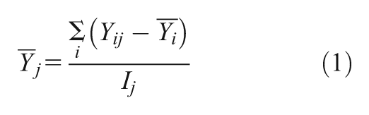
where Yij
is the observed outcome for student i in school j, and Ij
is the number of students in school j. Such unadjusted comparisons are the basis for most educational accountability systems, including those mandated by the No Child Left Behind Act (NCLB). Schools are grouped into categories and assigned ratings such as “school of excellence” or “low-performing school” based on transformations of Equation 1, such as the percentage of students who exceed some threshold score and pass the exam. If all students were randomly assigned to schools and compelled to stay enrolled in them,
Consider a general causal model for the impact of school attendance on student outcomes:

Following Raudenbush and Willms (1995), Equation 2 partitions the impact of school j on outcome Yij into school practices (Fj ) and school context (Cj ). Practices include factors under a school’s control, such as curriculum, administrative leadership, utilization of resources, and perhaps teacher quality. Context includes factors such as the demographic composition of the school and surrounding neighborhood that, according to Raudenbush and Willms (1995), are exogenous to the practices of schools’ administrators and teachers. Sij is a set of student-level characteristics, such as race, ethnicity, family income, and student ability, that have an independent influence on outcomes; uj and eij are school- and student-level error terms.
This model highlights a number of challenges for unbiased estimation of school value added. First, failure to account for all differences across schools in student-level characteristics would lead us to overestimate the effectiveness of schools that attract and retain “good” students and to underestimate the effectiveness of schools that attract and retain “bad” students. High-quality measures of student characteristics are thus critical for obtaining unbiased estimates of school value added. At the same time, treating within-school coefficients of student characteristics as fixed parameters may lead us to ignore the consequences of school-to-school differences in these coefficients, as we will explain in more detail.
Second, Raudenbush and Willms (1995) distinguish between Type A school effects, which estimate a school’s total contribution to student outcomes relative to an average school, and Type B school effects, which separate the impact of school practice from context. As Raudenbush and Willms note, perfect measures of Sij do allow us to estimate Type A school effects, because we do not need to decompose the contribution of practice and context to school value added. We can estimate Type A school effects using VAMs of the following form:

where Yijt is an outcome for student i in school j in year t; Sijt is a vector of student covariates, including prior years’ test scores and demographics; and vijt is an error term equal to σ j + θ t + ϵ ijt , where σ j is a school effect constant over time; θ t is a year effect constant across schools that incorporates year-specific shocks, such as changes in the test or in economic conditions; and ϵ ijt is an idiosyncratic student error term. For our purposes, the parameter of interest is the school effect σ j , which is the standard deviation of schools’ average effects on a given outcome after accounting for differences in students’ initial characteristics and statewide year effects.
We can estimate Raudenbush and Willms’s (1995) Type B models using the following equation:

where
We believe that the longitudinal data available in Massachusetts and Texas allow a better estimate of Type A effects than is usually available. Analyzing data from Charlotte-Mecklenburg, Deming (2014) demonstrates that nonexperimental estimates of school value added for four-year college attendance (i.e., Type A effects) match lottery-based estimates reasonably well. 8 Specifications that control for a student’s test score history and demographics do the best job of approximating experimental estimates, and this is the strategy we pursue here. Specifically, our VAMs control for sex, race/ethnicity, FRPL status, interactions between race/ethnicity and FRPL status, English language learner status (pre–high school), immigrant status, special education status (pre–high school), pre–high school seventh- and eighth-grade test scores and their squared and cubed terms, pre–high school attendance, interactions between race/ethnicity and FRPL status, and mean demographic and achievement composition of a student’s middle school. Nonetheless, our estimates are not based on random assignment, and they should not be interpreted as unbiased causal estimates. In further analyses, we bring in another data set to attempt to assess the impact of unobserved variables on our estimates of school effects.
For the reasons outlined earlier, estimating credible Type B school effects is more challenging. Nonetheless, a rigorous analysis of how school composition affects different outcomes is critically important, because it may yield insight into the mechanisms underlying our results. We thus make one further adjustment to the conventional VAM approach in Equation 3. When we estimate our school VAMs, we predict individual students’ performance from the individual-level coefficients in Equation 1 with high school fixed effects included. As a result, the coefficients in our prediction equation represent the weighted average of the within-school coefficients of student characteristics. Because we are interested in how much difference it makes for students to attend different high schools, the counterfactual is what would happen if students all attended identical high schools that were all like the average high school in their state.
At present, for example, black students are more likely to attend schools with above-average percentages of black students, and these schools tend to have below-average gains between 8th and 10th grade. Other disadvantaged groups face the same pattern. Suppose these schools have below-average gains because they have trouble attracting or retaining above-average teachers. If we regress 10th-grade scores on both race and 8th-grade scores, we are quite likely to find that being black has a significant negative effect on students’ gains during 9th and 10th grades, because attending a school with an unusually high fraction of black students tends to reduce all students’ gains. In this scenario, the between-school effect of being black could be negative even if the within-school effect of being black were zero. If we estimate VAMs by regressing 10th-grade scores on 8th-grade scores and race, the coefficient (effect) of being black will be the weighted average of the between- and within-school effects. This is not the best estimate for understanding how important it is to attend one high school rather than another, because in this hypothetical world, being black has no effect on a student’s gains in an average school; here, being black influences gains only because black students are more likely to attend schools with relatively ineffective teachers.
The most important implication of this scenario is that because our counterfactual is that all high schools in the same state have identical effects, the effect of an individual characteristic like 8th-grade test scores or race on 10th-grade test scores is, by definition, the average within-school effect of the characteristic. Of course, within-school effects of race may also reflect the influence of school practices, like tracking. We will return to this possibility.
Our analysis proceeds as follows. We first estimate high school effects on achievement and four-year college attendance using a variance decomposition that allows for a direct comparison of our results with previous work on school effects. Our estimates control for students’ pre–high school test performance, demographic information, and high school fixed effects, so we can also estimate the models described earlier. We estimate those models separately by state but pool data across cohorts within the same state. These models parallel the school effects literature, which generally controls only eighth-grade scores and demographic covariates (e.g., in studies based on the NELS).
We then compare the size of high school effects on test scores and educational attainment. While it is well-known that poor and minority students often attend schools with lower test score levels, we investigate whether these disadvantaged groups disproportionately attend high schools with lower average value added. This approach still makes the common-impact assumption—that schools have the same average impact on all types of students—which has not been adequately tested in the school-effects literature. To address this issue, we next investigate whether attending a high value-added school has equally beneficial effects on historically advantaged and disadvantaged students. To do this, we reestimate our VAMs using high school subgroups as the unit of analysis. Specifically, we classify students into one of four groups based on economic status (low income or higher income) and race/ethnicity (white versus black or Hispanic, which we refer to as “white or nonwhite”). 9 Figure 1 shows a simple matrix of student subgroups. We allow each high school to have as many separate value-added measures as it has subgroups that included 20 or more students in the two cohorts we study. A high school with 20 or more students in each of the four quadrants of Figure 1 can thus have four separate value-added measures.
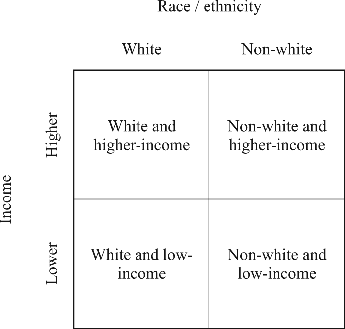
Matrix of student subgroups.
We then conduct a series of statistical tests that account for error dependence across students attending the same high school to determine (1) whether high school effects differ across groups within the same school and, (2) if they do differ, whether within-school differences are greater for college attendance or for test scores. We explicitly test for heterogeneity of effects by holding race constant and varying income status (down the columns of Figure 1) and by holding income status constant and varying race (across the columns of Figure 1).
Finally, we use these estimates to consider the combined implications of between- and within-school inequality for whether lower-income and nonwhite students attend high schools that are systematically more or less effective than the average school at promoting test score growth and college attendance among students like themselves.
Sensitivity Analysis
Because students are not randomly assigned to schools, a school’s value-added measures may be biased in the absence of robust controls for family background. Administrative data do not include detailed measures of family SES, so one central concern is that our conclusions might be different if we had access to a wider range of control variables. Online Appendix A shows results of a sensitivity analysis that addresses this question. Specifically, we calculate school value-added estimates using the NELS and compare estimates controlling only for eighth-grade test scores plus FRPL status to estimates that include more detailed indicators of SES. Including a more detailed set of SES measures does not, of course, rule out the possibility that our estimates of school effects are biased by the omission of other unobserved student and family characteristics. Nonetheless, in the absence of lottery data, we view this as the best currently available test for bias in value-added measures derived from administrative data.
We estimated multiple other specifications of our VAMs to determine how sensitive our results are to using within- versus between-school coefficients on individual demographic characteristics in our prediction equations, whether including high school SES and race compositional characteristics substantially alter our estimates (essentially, these are the Type B estimates discussed earlier), and whether including district fixed effects in our models substantially changes the inferences we would make about the magnitude of school effects or the relationship between school effectiveness and inequality. Our conclusions remained the same in each of these cases.
Results
Descriptive Statistics
Tables 1 and 2 describe the characteristics of the 118,276 Massachusetts students and 428,962 Texas students who entered ninth grade in a public school for the first time in 2003 or 2004. Students attending public schools in these two states are quite different from one another. Massachusetts ninth graders are substantially more likely than Texas ninth graders to be white (78 versus 45 percent). Massachusetts has roughly equal proportions of black and Hispanic students (7 and 10 percent, respectively). In Texas, 14 percent of students are black and 38 percent are Hispanic. Using eligibility for free or reduced-price school meals as an income proxy, we found that Massachusetts students are also somewhat more affluent. Only 32 percent of public high school students qualified for FRPL in Massachusetts, compared to 41 percent in Texas. (These poverty rates probably overstate the actual difference in living standards between the two states, because housing costs are much higher in Massachusetts than in Texas.)
Descriptive Statistics by Race.
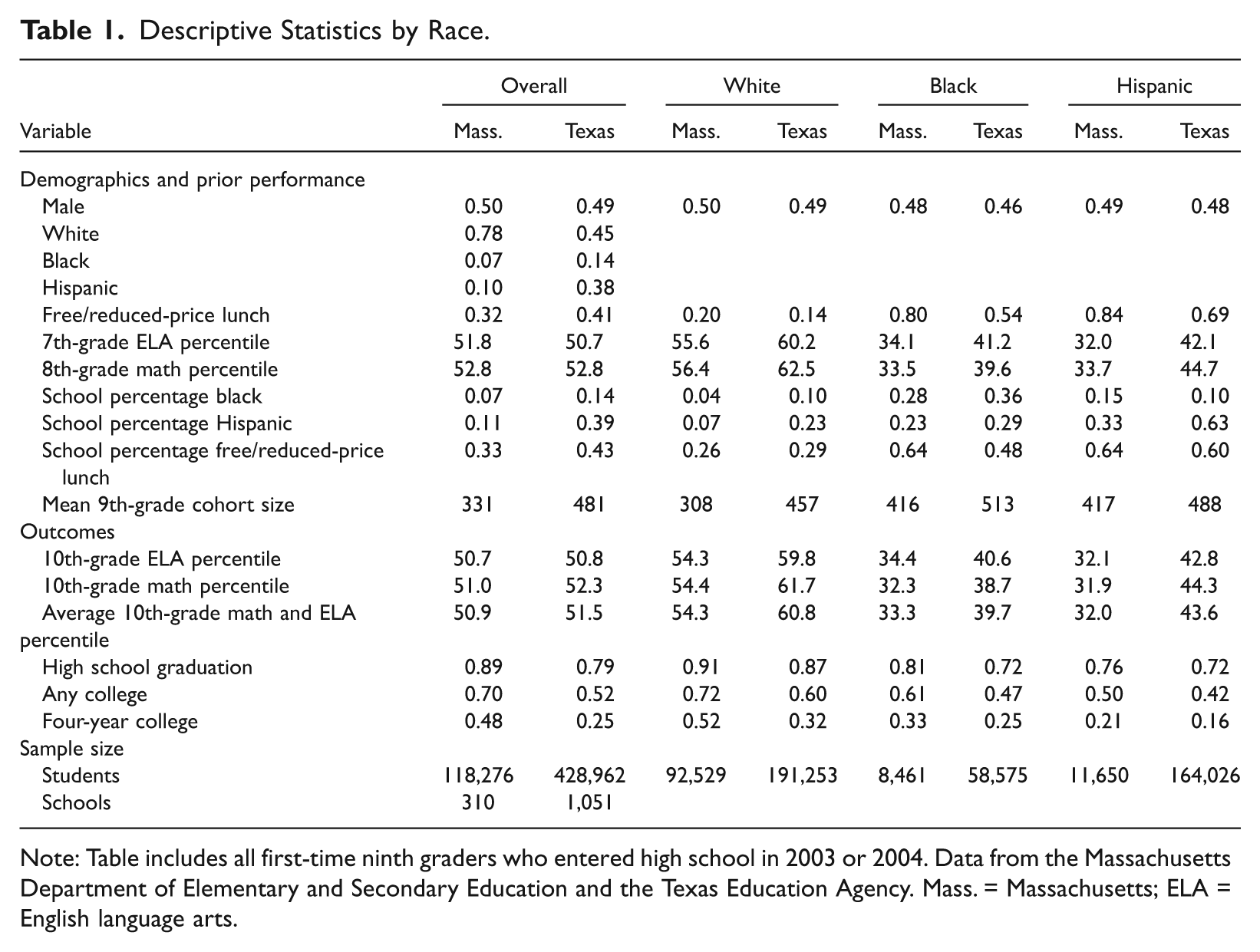
Note: Table includes all first-time ninth graders who entered high school in 2003 or 2004. Data from the Massachusetts Department of Elementary and Secondary Education and the Texas Education Agency. Mass. = Massachusetts; ELA = English language arts.
Descriptive Statistics by Income.
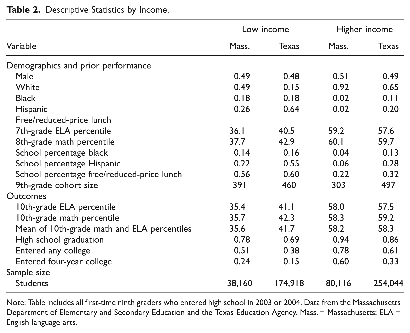
Note: Table includes all first-time ninth graders who entered high school in 2003 or 2004. Data from the Massachusetts Department of Elementary and Secondary Education and the Texas Education Agency. Mass. = Massachusetts; ELA = English language arts.
In Massachusetts and Texas, students’ academic performance varies substantially by race and income. Tables 1 and 2 show student test scores in percentiles. 10 The average black student enters high school with math scores 23 percentiles below the average white student in both Texas and Massachusetts. But the initial gap between Hispanics and whites is only 18 percentiles in Texas, compared to 23 percentiles in Massachusetts. When we combine the ELA and math results, the average test score gap between low-income and higher-income students is also smaller in Texas (17 percentiles) than in Massachusetts (23 percentiles).
In Massachusetts, 89 percent of our sample graduated from a Massachusetts high school in four years, compared to 79 percent in Texas; and 48 percent of students who reached 10th grade in Massachusetts attended a four-year college, compared to 25 percent in Texas.
Racial and income gaps in educational attainment are large in both states, but income gaps in educational attainment are larger than racial gaps. In Massachusetts, white students are 19 percentage points more likely than black students, and 31 percentage points more likely than Hispanic students, to attend a four-year college; the gap between low- and higher-income students is 36 percentage points. In Texas, the black-white gap in four-year college entry is 7 percentage points, the Hispanic-white gap is 16 percentage points, and the gap between low- and higher-income students is 18 percentage points.
How Large Are Differences Between High Schools?
Tables 3 and 4 show the share of the total variation in test scores explained by schools for the 2003 and 2004 cohorts combined. Table 3 displays the standard deviations of high schools’ estimated effects, both unconditionally (levels) and conditional on pre–high school characteristics (value-added). Table 4 uses data in Table 3 to calculate the fraction of the total variance between and within schools for levels and value added.
Standard Deviations of Levels and Value-added Distributions for High Schools.
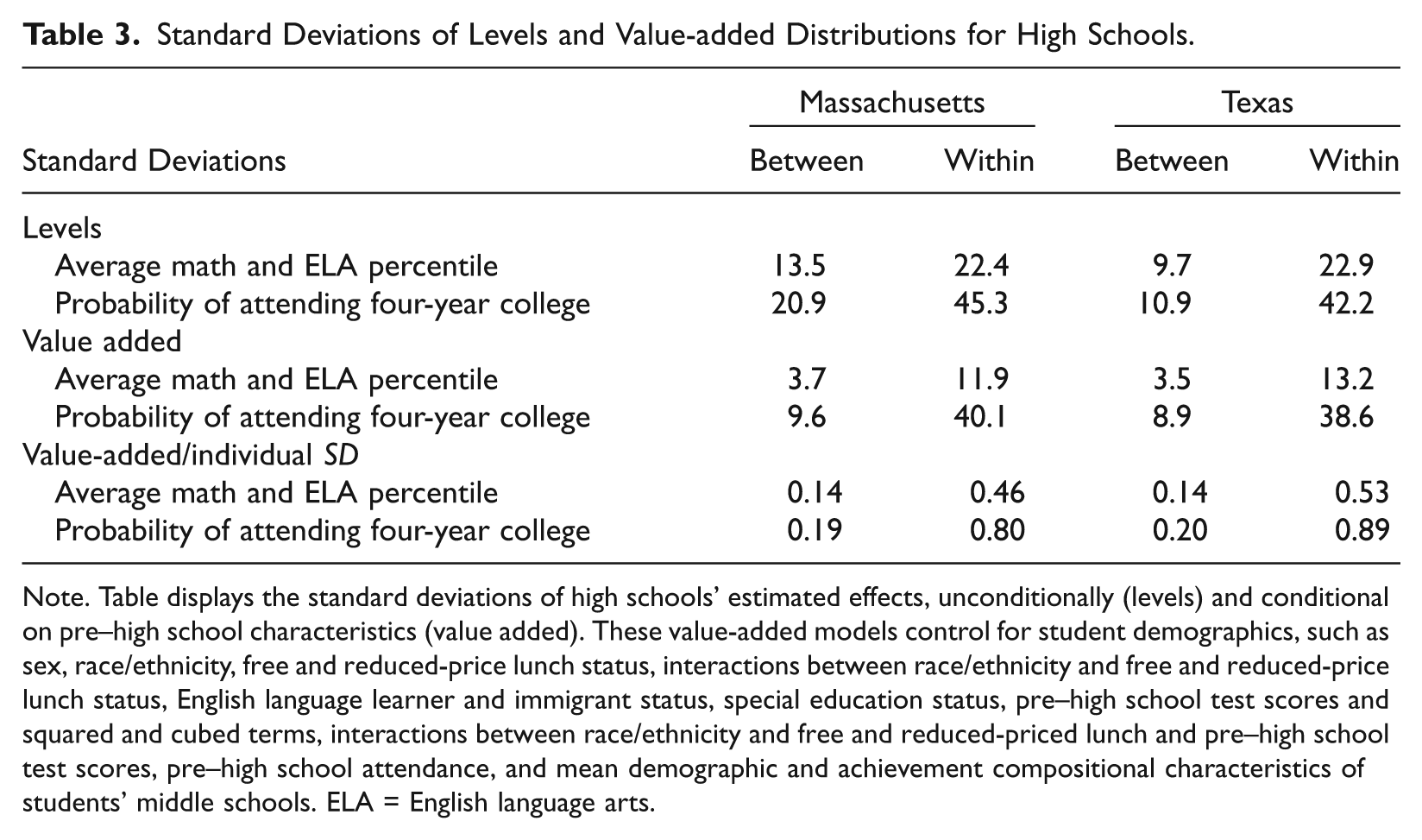
Note. Table displays the standard deviations of high schools’ estimated effects, unconditionally (levels) and conditional on pre–high school characteristics (value added). These value-added models control for student demographics, such as sex, race/ethnicity, free and reduced-price lunch status, interactions between race/ethnicity and free and reduced-price lunch status, English language learner and immigrant status, special education status, pre–high school test scores and squared and cubed terms, interactions between race/ethnicity and free and reduced-priced lunch and pre–high school test scores, pre–high school attendance, and mean demographic and achievement compositional characteristics of students’ middle schools. ELA = English language arts.
Variance Decompositions of Levels and Value-added Distributions for High Schools (in percentages).
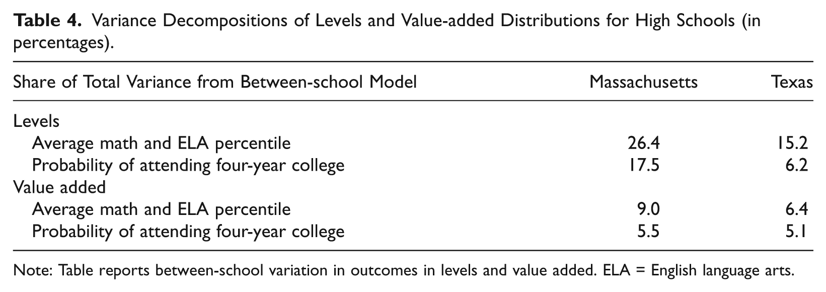
Note: Table reports between-school variation in outcomes in levels and value added. ELA = English language arts.
Using variation in schools’ mean level of achievement to measure inequality, Massachusetts high schools look considerably more unequal than Texas high schools. Differences in high schools’ mean 10th-grade achievement account for 26 percent of the total variance in Massachusetts, compared to only 15 percent in Texas. Table 3 shows that the standard deviation of high schools’ mean 10th-grade achievement is 13.5 percentiles in Massachusetts versus 9.7 percentiles in Texas—a difference of 39 percent. However, when we use value added to measure high school quality, the dispersions in Massachusetts and Texas are almost identical (SD = 3.7 percentiles in Massachusetts versus 3.5 percentiles in Texas). This contrast tells us that Massachusetts high schools are more unequal than Texas high schools because the 9th graders who enter different Massachusetts public high schools have more unequal scores than do those who enter different Texas high schools, not because Massachusetts high schools have more unequal effects on 9th and 10th graders. This demonstrates why our preferred specification is the VAM, which gives schools credit or blame for how well their students perform relative to students with similar characteristics who attend the average Massachusetts or Texas school.
Just as with test scores, high schools’ unadjusted college entrance rates are more unequal in Massachusetts (SD = 20.9 percentage points) than in Texas (SD = 10.9 percentage points). But once again, this is because ninth graders entering different Massachusetts high schools are more unequal than those entering different Texas high schools. Once we look at value added, the standard deviations of schools’ estimated effects are quite similar (9.6 percentage points in Massachusetts versus 8.9 points in Texas).
We turn now to the more difficult question of whether differences in high school quality have more influence on a student’s chances of attending a four-year college or a student’s 10th-grade test scores. Answering this question requires a common metric. One strategy is to standardize both measures by dividing them by the overall standard deviation for individuals in each state. Table 3 shows results of this calculation. A one–standard deviation improvement in high school value added raises students’ 10th-grade achievement by 0.14 standard deviations in both Massachusetts and Texas. For college attendance, a one–standard deviation increase in high school value added raises students’ chances of attending a four-year college by 0.19 standard deviations in Massachusetts and .20 standard deviations in Texas. Using this metric, disparities in high school value added are almost identical in Texas and Massachusetts and are larger for college entrance rates than for academic achievement gains in both states.
Another way to think about the relative impact of high school value added on test scores and college attendance is to compare the estimated effect of attending a high school one standard deviation above the state average to the effect of coming from a family that is above rather than below the cutoff for FRPL. For test scores, the effect of attending the better high school is 16 percent of the gap between low- and higher-income students in Massachusetts and 21 percent of the gap in Texas. When we look at the effect of attending a high school one standard deviation above the mean on sending students to four-year colleges, the effect is 28 percent of the gap between low- and higher-income students in Massachusetts and 49 percent of the gap in Texas. These comparisons also suggest that attending an unusually effective high school has more impact on the fraction of students entering a four-year college than on test score gains during 9th and 10th grades.
One potential concern with these value-added estimates is that although we are able to control for prior test scores, these scores predict 10th-grade scores better than they predict college attendance. One might expect our VAMs for college attendance to make more accurate predictions if we had a good measure of entering 9th graders’ college plans and aspirations and their parents’ commitment to supporting these plans. Massachusetts asks 8th graders how much schooling they expect to get, but responses to this question do not improve our ability to predict college attendance five years later, because 94 percent of all Massachusetts 8th graders say they expect to attend college.
In an effort to determine how much our results might change if we had more precise measures of students’ family income and their parents’ educational attainment, family size, and marital status, we turned to the 1988 NELS. Online Appendix A summarizes our findings. Including a more precise measure of parental income, plus measures of fathers’ and mothers’ educational attainment, family size, and whether the family head was a single parent reduced the estimated standard deviation of school effects by 1.8 percent for 10th-grade reading, 2.4 percent for 10th-grade math, and 0.7 percent for attending a four-year college. 11 Some of the apparent variability of high schools’ impact on college attendance is indeed due to unmeasured socioeconomic differences among high schools’ entering 9th graders, but correcting the problem strengthens the claim that high schools’ effects on college attendance are typically larger than their effects on reading or math scores.
One hypothesis to explain this, which we cannot test here, is that high school students can change their college plans more easily than they can change their math or reading skills. Alexander and Eckland’s (1975) study, for example, found a correlation of only 0.40 between students’ college plans in 10th and 12th grades. The correlation between achievement scores over time is substantially higher. As a result, we infer that peers, teachers, and counselors have more influence over whether high school students attend college than over their reading or math test scores.
Do High Schools Increase or Reduce Racial and Socioeconomic Differences?
What do these estimates imply about whether high schools reduce the impact of family background, increase it, or leave it unchanged? Table 5 uses estimates from Table 3 to calculate the value added by the high school attended by the median student in various groups along with the difference in quality between high schools attended by traditionally advantaged and disadvantaged groups. Positive numbers represent advantages for white or higher-income students.
Between-group Differences in Value Added at the School Attended by the Median Student, Using Common Impact Assumption.
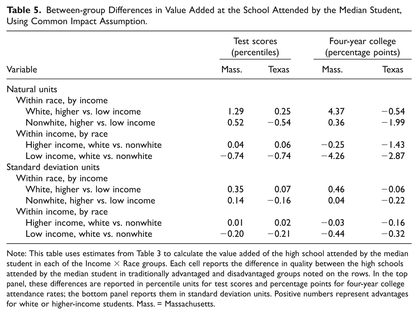
Note: This table uses estimates from Table 3 to calculate the value added of the high school attended by the median student in each of the Income × Race groups. Each cell reports the difference in quality between the high schools attended by the median student in traditionally advantaged and disadvantaged groups noted on the rows. In the top panel, these differences are reported in percentile units for test scores and percentage points for four-year college attendance rates; the bottom panel reports them in standard deviation units. Positive numbers represent advantages for white or higher-income students. Mass. = Massachusetts.
Table 5 paints a mixed picture about schools’ effects on race and income-based inequality. We do not observe a clear pattern of historically advantaged groups (white or higher-income students) attending higher-quality high schools. The historically advantaged group has a school quality advantage in only 9 of the 16 cells, and these differences are often very small. Our analyses suggest that high school effects are larger for college attendance than for test scores, but no group appears to be systematically advantaged.
How Large Are Differences within High Schools?
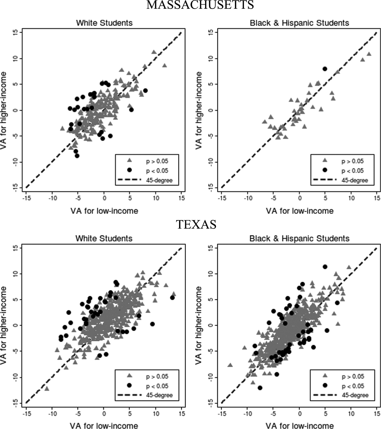
Estimates in Tables 3, 4, and 5 implicitly assume that all student groups benefit equally from attending a high-value-added school. The treatment effect could, however, vary systematically within high schools, with historically disadvantaged students benefiting less than their more advantaged classmates from higher-value-added schools. To test for this possibility, we reestimate our VAMs using school subgroups as the unit of analysis and allowing for as many separate value-added measures as there are race-by-income combinations. We first statistically test whether high school effects differ consistently for student subgroups within the same schools. Then we test whether there is more within-school divergence between subgroups for college attendance than for test scores. Figures 2 and 3 present results of these statistical tests for differences between subgroups and for variation across subgroups in how much high schools affect different outcomes. Figure 2 compares results for test scores in both states; Figure 3 shows results for college attendance. Table 6 shows regression results that quantify these within-school differences. Because of racial and income segregation, many high schools do not have enough students in all four subgroups to make reliable estimates for every subgroup. For example, only 71 percent of high schools in Massachusetts and 44 percent of high schools in Texas are included in the figure comparing value added for low- and higher-income white students. Table 6 shows the number of high schools included in each analysis.
Do the effects of high schools on test scores vary by student group? Within-race comparisons of school test score value added, estimated separately for higher- and low-income students.
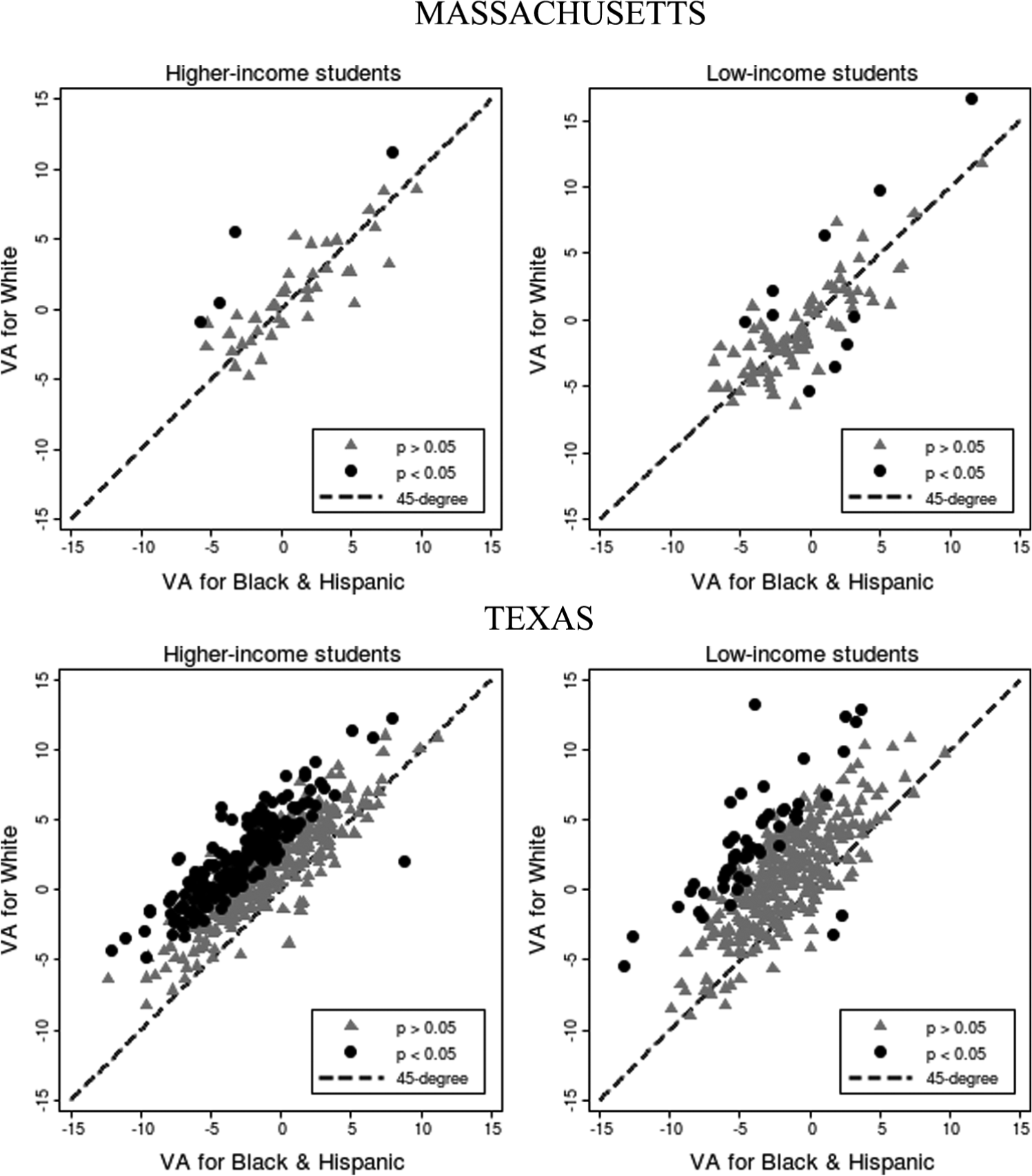
Do the effects of high schools on test scores vary by student group? Within-income comparisons of school test score value added, estimated separately for white and black/Hispanic students.
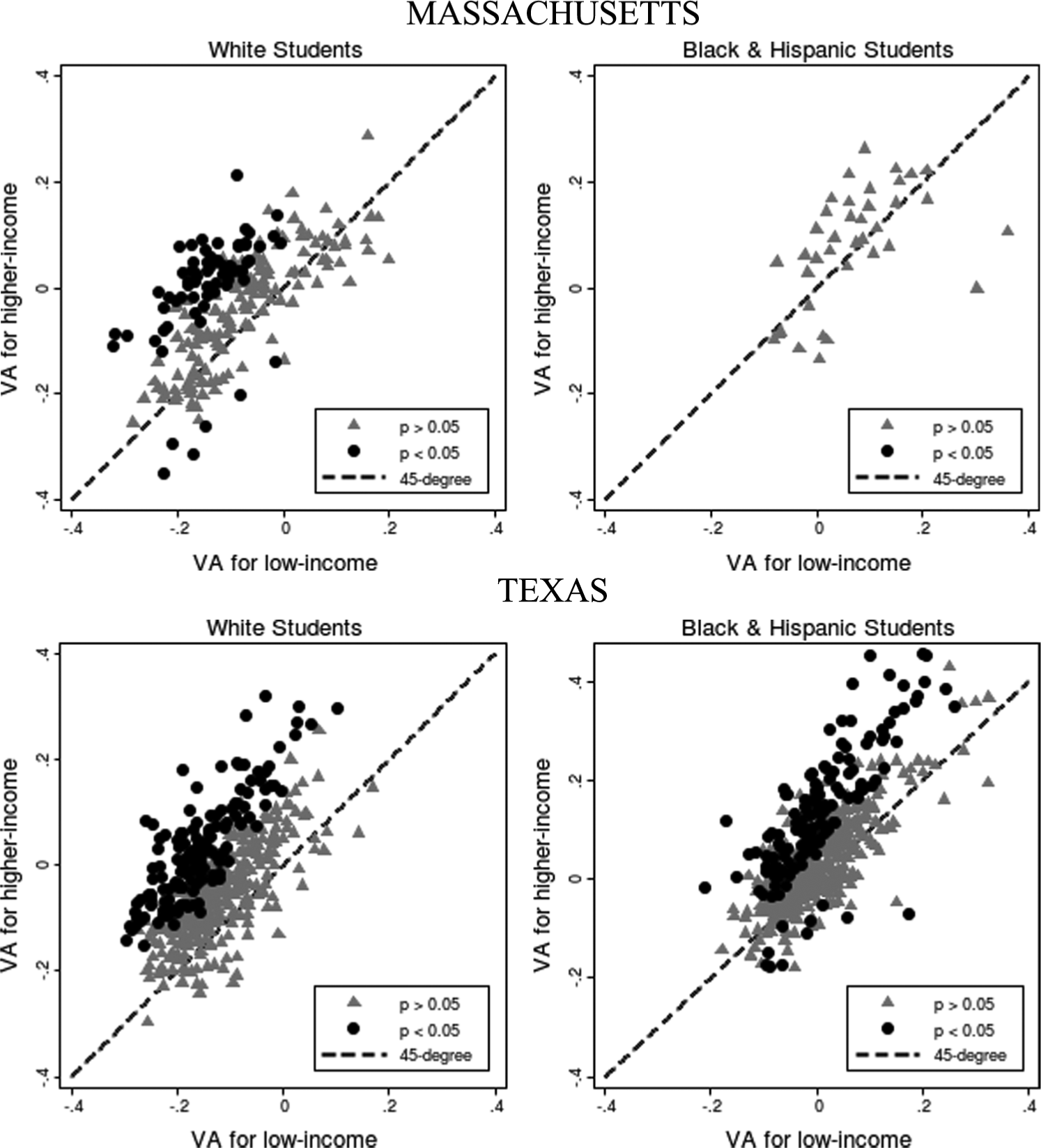
Do the effects of high schools on college attendance vary by student group? Within-race comparisons of school value added to four-year college attendance, estimated separately for higher- and low-income students.
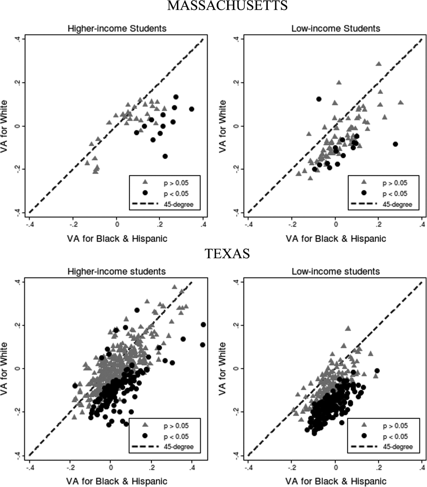
Do the effects of high schools on college attendance vary by student group? Within-income comparisons of school value-added to four-year college attendance, estimated separately for white and black/Hispanic students.
Regressions Estimating Within-school Heterogeneity of School Effects.
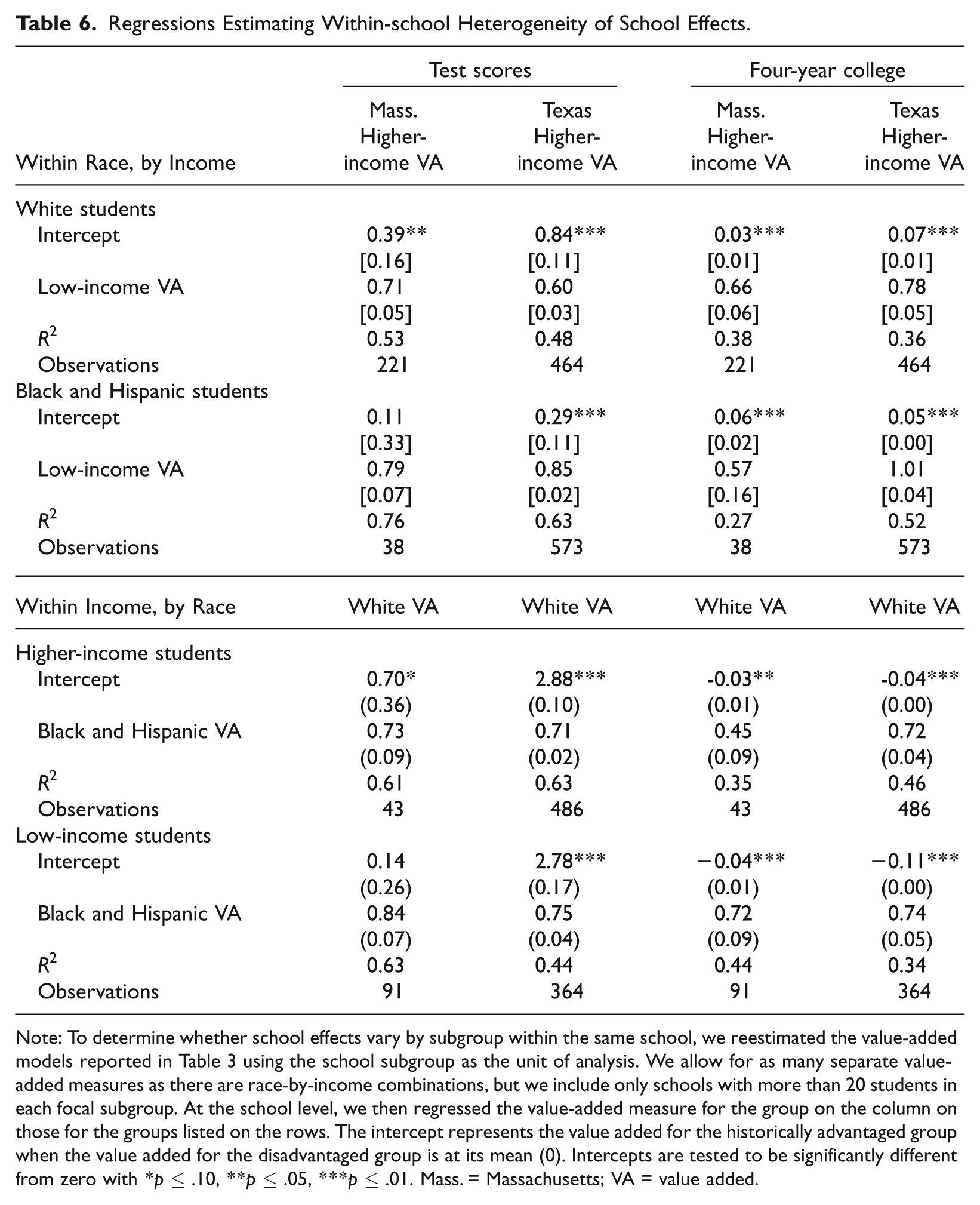
Note: To determine whether school effects vary by subgroup within the same school, we reestimated the value-added models reported in Table 3 using the school subgroup as the unit of analysis. We allow for as many separate value-added measures as there are race-by-income combinations, but we include only schools with more than 20 students in each focal subgroup. At the school level, we then regressed the value-added measure for the group on the column on those for the groups listed on the rows. The intercept represents the value added for the historically advantaged group when the value added for the disadvantaged group is at its mean (0). Intercepts are tested to be significantly different from zero with *p ≤ .10, **p ≤ .05, ***p ≤ .01. Mass. = Massachusetts; VA = value added.
Figure 2a plots high schools’ estimated value added for test scores for higher- versus low-income students of the same race in each state; Figure 2b compares white and nonwhite students in the same income group in each state. Figures 3a and 3b follow the same structure but change the outcome of interest to four-year college attendance. Each point on the scatterplot represents one high school. The dashed line is the 45-degree line. If both groups within a high school have equal value added, the point for the school will fall on the 45-degree line. Schools where advantaged students have higher gains than disadvantaged students fall above the 45-degree line. Schools in which advantaged students have lower gains than disadvantaged students fall below the 45-degree line. Bold points represent schools where the probability that the true difference between the two groups has the same sign as the observed difference exceeds .95. Larger vertical distances between the observations and the 45-degree line indicate larger differences in a school’s effect on the two groups. The notes for each figure give the probability (based on an F test) that all deviations from the 45-degree line are due to chance.
Three major findings emerge from Figures 2 and 3. First, even when students from different economic or racial backgrounds attend the same high school, there are often systematic differences in how much they benefit from the school. Second, these differences are much more pronounced for college attendance than for test scores. For test scores, the differences in value added between traditionally advantaged and disadvantaged students in the same high school are seldom significant. The exception is that white students in Texas gain substantially more than nonwhites in the same school and income group. However, when we turn from test scores to college attendance, we can strongly reject the hypothesis that high schools have the same impact on low-income and higher-income students, and this is true among white and nonwhite students. The magnitude of these differences is usually large and indicates substantial school-to-school differences in how schools affect different groups’ chances of attending a four-year college.
Table 6 quantifies these differences. The intercept represents the within-school difference in a school with average value added for the group on the x-axis. In high schools where low-income whites have average college attendance value added, higher-income whites are about 3 percentage points more likely to attend college in Massachusetts and 7 percentage points more likely to do so in Texas. Among nonwhite students, higher-income students have an advantage of 6 percentage points in Massachusetts and 5 percentage points in Texas. The within-school gaps for college value added dwarf those for test score value added. The point estimates for racial differences in test score value added are less than 1 percentile.
The third major finding in Figures 2 and 3 is that while low-income students are less likely to attend college than higher-income students of the same race who had the same eighth-grade test scores and attended the same high school, this pattern does not hold when we compare nonwhite to white students. Nonwhite students are more likely to attend a four-year college than white students in the same high school who entered ninth grade with the same test scores and came from the same income group. The intercepts in Table 6 show that among higher-income students attending the same school in Massachusetts, nonwhites are 3 percentage points more likely than initially similar whites to attend a four-year college. In Texas, nonwhites are 4 percentage points more likely than economically and academically similar whites to attend a four-year college. Among low-income students, nonwhites have a 4–percentage point advantage in Massachusetts and an 11–percentage point advantage in Texas.
How Do Differences between and within Schools Together Affect Racial and Socioeconomic Inequality?
Figure 2, Figure 3, and Table 6 summarize outcomes for students who attend the same high school but include only schools that have sufficient numbers of students in each subgroup. However, they do not account for inequalities that arise because students from different social backgrounds are likely to attend different schools. To address this issue, we reestimated VAMs for all schools, allowing for up to four separate value-added estimates per school. These estimates effectively combine within- and between-school differences to estimate the total difference between subgroups in average value added to test performance between 8th and 10th grades. Table 7 quantifies these differences by showing racial and income-based differences in overall school value added for the median student in each subgroup.
Between-group Differences in Value Added at the School Attended by the Median Student, Using Heterogeneous Treatment Effects Assumption.
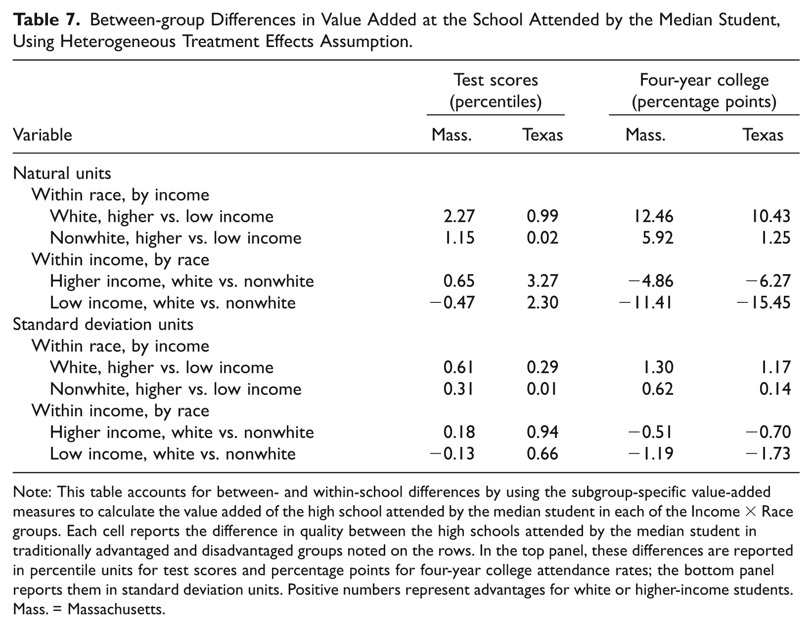
Note: This table accounts for between- and within-school differences by using the subgroup-specific value-added measures to calculate the value added of the high school attended by the median student in each of the Income × Race groups. Each cell reports the difference in quality between the high schools attended by the median student in traditionally advantaged and disadvantaged groups noted on the rows. In the top panel, these differences are reported in percentile units for test scores and percentage points for four-year college attendance rates; the bottom panel reports them in standard deviation units. Positive numbers represent advantages for white or higher-income students. Mass. = Massachusetts.
Massachusetts
When we look at total disparities in high schools’ value added to 10th-grade test scores in Massachusetts, only one of the four comparisons in Table 7 shows a statistically significant difference. The exception is that in Massachusetts, the median higher-income white student attends a school that raises his or her 10th-grade achievement scores 2.3 percentiles more than the school that the median low-income white student attends. In contrast, when we look at the chances of entering a four-year college, the median higher-income white student in Massachusetts attends a high school where higher-income whites are 12 percentage points more likely than low-income whites with the same 8th-grade achievement scores to attend a four-year college. This pattern holds among nonwhites, although the difference is only half as large. When we compare Massachusetts whites to nonwhites in the same income group and with the same 8th-grade test scores, however, white students are less likely than similar nonwhite students to attend schools that produce higher-than-expected college entrance rates.
Texas
The Massachusetts pattern is reversed in Texas. We find little difference by income in high schools’ mean value added to test scores, but we find substantial differences by race among both higher- and low-income students with similar test scores. Among higher-income students, the median nonwhite student attends a school that is 3.3 percentiles less effective at raising test scores than the school attended by his or her white counterparts. The same racial difference is apparent among low-income students in Texas. In summary, when it comes to test scores, race appears to play a greater stratifying role in Texas, whereas family income matters more in Massachusetts.
However, differences between high schools have a more pronounced effect on subgroup differences in college attendance than in test performance. This pattern holds in both Texas and Massachusetts. Higher-income Texas students attend schools where high-income students attend four-year colleges at higher rates than we would expect based on their eighth-grade characteristics. Likewise, nonwhite students in Texas, like their counterparts in Massachusetts, are more likely to attend high schools where college attendance is more common among nonwhite than white students in the same income group with similar eighth-grade achievement scores.
We can now ask what the results in Table 7 imply for the question of whether schools reduce the effects of family background on children’s life chances. One answer, of course, is that they do not imply anything about the effects of schools in general, because they take everything that happens before ninth grade as given, including large economic and racial disparities in academic achievement among eighth graders. That means we must recast the question by asking what these estimates imply about the effects of public high schools on economic and racial disparities in student outcomes. Table 5 shows that under the common-impact assumption, low-income and nonwhite students in Massachusetts and Texas attend high schools of quite similar average quality. However, Table 7 shows that high schools in both states appear to reduce racial inequality in college attendance, because the median nonwhite student attends a school in which nonwhites are more likely to attend college than are whites with similar initial characteristics. Among higher-income students in Massachusetts, school effects on college attendance are 5 percentage points more favorable for black and Hispanic students than for whites. For low-income students, that difference is even larger—about 11 percentage points. Among higher-income students in Texas, school effects on college attendance are 6 percentage points more favorable for black and Hispanic students than for white students. For low-income students, that difference is substantially larger—about 15 percentage points.
To be clear, these findings do not imply that nonwhites are more likely than whites to attend a four-year college. They imply only that when white and nonwhite students enter high school with similar achievement and other covariates, their college attendance rates differ less than we would expect based solely on their academic skills at the end of eighth grade. Furthermore, while this could be a school effect, we have no way of knowing whether it reflects differences in the way white and nonwhite students are treated, or treat one another, in school. If low-income black students are more optimistic than low-income white students about the returns to staying in school, or more pessimistic about their chances of finding a steady blue-collar job that pays a living wage, for example, we have no way of determining where such a difference came from in our data.
However, the opposite is true for lower-income students. Lower-income students are concentrated in high schools where income-based inequality in college attendance is greater than at the average high school. Taking between- and within-school inequality into account, school effects on college attendance are 12 percentage points more positive for higher-income than for low-income whites and 6 percentage points more positive for higher-income versus low-income minorities in Massachusetts. We observe similar patterns in Texas.
Comparing Tables 5 and 7 demonstrates that we should not assume high schools have a similar effect on all students who attend them. That assumption can lead to erroneous conclusions about whether students from different backgrounds attend equally effective schools. The estimated effects of high schools in Table 7, which account for systematic differences within schools, are almost all larger than those in Table 5, which ignore within-school differences. Ignoring within-school inequality can thus make opportunities for different groups look more equal than they are. Because gaps within schools are greater for college attendance than for test scores, ignoring differences within high schools in different groups’ college entrance rates is particularly likely to distort inferences about high schools’ role in explaining eventual educational attainment. Table 5, which considers only differences between high schools, shows only a 4.4–percentage point difference in college attendance between low- and higher-income whites in Massachusetts. In Table 7, which factors in differences within those same high schools, the gap increases to 12.5 percentage points. Results in Texas are similar.
The most notable exception to this pattern is for racial differences within income groups for college attendance (the lower-right panel of Tables 5 and 7). When we focus on between-school variation, the high schools that nonwhite students attend have somewhat higher mean value added for college attendance than do the high schools that white students in the same income group attend. Once we incorporate within-school inequality into our analyses, nonwhites increase their advantage over whites in the same income group with similar achievement scores. Overall, comparing these two methods for estimating school effects shows that ignoring within-school heterogeneity can understate inequality, both when traditionally advantaged groups have the advantage and when traditionally disadvantaged groups have the advantage.
Conclusions
Since the Coleman Report, one of the most consistent findings in the sociology of education is that differences in test performance are within, rather than between, schools. This finding is sometimes translated to mean that schools “don’t matter” much for the intergenerational transmission of advantages and disadvantages. Yet Coleman himself acknowledged the limitations of examining test scores alone. His report includes a seldom-quoted “cautionary word” that test scores “are not the only results of schooling, but simply the most tangible ones” and the report’s results should be understood as “partial and incomplete” (Coleman et al. 1966:273). Using a data set linking all Massachusetts and Texas students entering public high schools in 2003 and 2004 to their characteristics prior to high school and their college attendance after high school, we show that differences between schools are more important for college attendance than for test scores.
In addition, we show that within-school differences play a powerful role in shaping outcomes for students from different backgrounds, and these effects vary across schools and outcomes. These within-school differences do not always work in the expected direction. We find that nonwhite students have a within-school advantage in four-year college attendance (net of their pre–high school characteristics), whereas lower-income students are even more disadvantaged within schools when we look at college attendance rather than achievement scores. Overall, we find that both between- and within-school inequalities widen gaps by income status, and these effects are particularly large for college attendance. Our results show that in the twenty-first century, low income is more of a disadvantage than race among high school students. We hasten to add, however, that this conclusion may not apply to elementary or middle schools (Condron 2009; Downey et al. 2004).
Our findings demonstrate that the inferences social scientists draw about the importance of going to one school versus another and the way opportunities are distributed within schools vary depending on which outcomes they study. If this is true, research on school effects needs to investigate a much broader array of outcomes than it has in the past. Although sociologists have long pointed out that the production of student outcomes involves the complex interaction of student and family characteristics, school resources (including the composition of the student body), and organizational practices, such as tracking, they usually stop short of investigating whether these interactions mean that different schools maximize different outcomes or maximize the outcomes of different kinds of students. For half a century, sociologists have demonstrated that different student groups within schools are differentially exposed to key resources and get different returns to these resources. However, the quantitative literature on the size of school effects seldom incorporates this insight into its models to clarify why schools have systematically different effects across groups and outcomes. We believe that an accurate picture of schools’ contribution to inequality requires us to relax the assumption that “good” schools have a common impact on all outcomes or all kinds of students.
Parents, citizens, and policy makers care about a much wider range of outcomes than those considered in the school-effects literature or in most school accountability systems. We hope our findings will stimulate others to estimate school effects for more of these outcomes. We also hope the evidence in this article will spur others to investigate new ways of analyzing school outcomes. Administrative data like those used in our study should make it possible to estimate school effects on almost any outcome for which a state collects data. States could—and we believe should—augment their educational databases with data from other administrative sources, including earnings information, vital statistics, and law enforcement records, to make such research possible.
These results have important implications for current education policy. As a result of NCLB, schools across the country have been required to make “adequate yearly progress” in increasing reading and math proficiency rates on state tests and to reduce achievement gaps between racial and socioeconomic groups. State waivers now override some of the key provisions of NCLB, but its key tenets—annual measurement of reading and math scores—remain in place. The common theme across these school and teacher accountability policies is strong reliance on test scores as the key measure of educational productivity. Our results suggest that examining schools’ effects on test scores alone may miss important ways in which schools improve (or hurt) their students’ life chances. Moreover, to the extent that school effects on test score and non–test score outcomes are weakly correlated, using test scores alone to evaluate schools will likely penalize a substantial number of schools that are effective at promoting other attainment-related outcomes and reward many other schools that are ineffective at promoting these outcomes.
Finally, we must once again emphasize that this study has a number of important limitations. First, our findings do not show what role formal education as a whole plays in the perpetuation of racial or economic disadvantages across generations, because they do not tell us what role preschools, elementary schools, and middle schools play in the test score disparities among eighth graders that explain so much of the variation in subsequent outcomes. Other studies of test score growth suggest, for example, that elementary schools tend to widen racial inequalities while reducing socioeconomic inequalities (Condron 2009; Downey et al. 2004).
Second, while we find that nonwhite students are more likely to attend a four-year college than are white students who enter the same high school with the same eighth-grade achievement scores and family income, we cannot identify the reasons for this difference with our data. Nonwhites could be more likely to attend college because the economic prospects for nonwhite high school graduates are so dismal. (Even among college graduates, nonwhites earn less than whites, but the ratio of nonwhite to white earnings is higher among college graduates than among high school graduates.) Nonwhites may also be more likely to attend college because of a frog pond effect, in which nonwhites attend less competitive high schools than whites with similar eighth-grade scores, making the nonwhites more academically self-confident. Nonwhites may also benefit from aggressive college recruitment aimed at attracting a more diverse student body. None of these possibilities implies that race no longer matters. Even in the 1980s, racial disparities in college attendance among students with similar test scores favored blacks, not whites (Neal and Johnson 1996). The black-white test score gap has narrowed over the past 40 years but not by much (Magnuson and Waldfogel 2008), and the ratio of black to white median family income was no higher in 2008 than in 1968 (Bloome 2014).
Finally, in this paper, we do not address the question of whether high schools currently provide students with equal opportunities. Policy makers who want schools to equalize opportunity often argue that in societies where children from different racial and economic backgrounds enter school with different skills, schools should assume responsibility for eliminating these group differences. Schools should, in other words, define equal opportunity in compensatory terms, seeking to boost test scores and educational attainment more among groups that start off at a disadvantage. Our VAMs, in contrast, assess each school’s effectiveness by asking whether its students fare better or worse than students with similar initial characteristics who attend different schools in the same state. We define schools serving advantaged and disadvantaged students as equally effective if they raise their students’ average math score or alter their students’ average probability of attending a four-year college by the same amount. This is a useful and legitimate measure of schools’ effectiveness, but it is not a measure of whether schools equalize opportunity, at least if that term means schools should be held responsible for offsetting the cost of having been born into a disadvantaged family. On the contrary, if schools boost advantaged and disadvantaged students’ test scores by the same amount, or alter their probability of attending a four-year college by the same amount, students will leave school as unequal as when they entered.
Research Ethics
Our research involves analysis of secondary data. In the case of Texas, all identifiers were stripped from the dataset before the researchers had access to the data. In the case of Massachusetts, the researchers analyzed the data under the auspices of a confidentiality agreement between Harvard University and the Massachusetts State Department of Education. All identifiers were stripped from the file prior to analysis. Data from Massachusetts were handled in such a way as to protect students’ privacy and confidentiality. This included storing these data on a secure Harvard-MIT Research Computing Environment server and requiring each researcher working with the data to sign a confidentiality affidavit.
Footnotes
Acknowledgements
The authors thank Carrie Conaway, Mike McPherson, Luke Miller, Aaron Pallas, Steve Raudenbush, and Rich Shavelson for their helpful comments on earlier drafts; the Massachusetts Department of Education, the Texas Education Agency, and the University of Texas at Dallas Education Research Center for providing access to the data; and the Spencer Foundation for its support. The conclusions of this research do not reflect the opinion or official position of the Massachusetts Department of Education, the Texas Education Agency, the Texas Higher Education Coordinating Board, or the State of Texas.
Notes
Author Biographies