A new method using the convolutional neural network with compressive sensing for fabric defect classification based on small sample sizes

Abstract

The convolutional neural network (CNN) has recently achieved great breakthroughs in many computer vision tasks. However, its application in fabric texture defects classification has not been thoroughly researched. To this end, this paper carries out a research on its application based on the CNN model. Meanwhile, since the CNN cannot achieve good classification accuracy in small sample sizes, a new method combining compressive sensing and the convolutional neural network (CS-CNN) is proposed. Specifically, this paper uses the compressive sampling theorem to compress and augment the data in small sample sizes; then the CNN can be employed to classify the data features directly from compressive sampling; finally, we use the test data to verify the classification performance of the method. The explanatory experimental results demonstrate that, in comparison with the state-of-the-art methods for running time, our CS-CNN approach can effectively improve the classification accuracy in fabric defect samples, even with a small number of defect samples.

Keywords

convolutional neural network compressive sensing fabric defects small sample sizes classification

In the textile industry, fabric defects represent an important problem in the quality control of textile manufacturing. Fabric defect detection and classification are the main methods used to ensure the quality of the fabric. Fabric defect classification is a vitally important process in the fabric quality evaluation, which can provide the defect information needed to adjust the machines and improve the processing technology. In the field of computer vision, the study of fabric defects has been a hot topic, which covers defect classification,^1,2 detection³ and recognition.⁴ Conventionally, fabric defects are evaluated by visual inspections of trained workers in accordance with human-made classification standards. Fabric defect classification remains a research issue and faces some difficulties due to the following three reasons. Firstly, new classes of fabric defects may be introduced with the growing application of fabric. Secondly, the similarities among different classes of fabric defects and the intra-class diversities of fabric defects make their discriminations challenging. Finally, different fibers, patterns and organizations of fabrics also make defect classification difficult.

New methods of fabric defect classification are springing up with developments in information science and computer vision. In these approaches, techniques used to extract image features include statistical procedures and Fourier transforms,⁵ the wavelet transform and dual-side co-occurrence matrix (GLCM)^6,7 and the Dempster–Shafer theory.⁸ Zhang et al.⁹ presented a scheme combining Gabor filters and the Gaussian mixture model (GMM) for defect detection and classification. In the detection task, texture features were extracted by using Gabor filters. In the classification task, a classifier based on the GMM was trained and it assigned each defect image to known classes. The experimental results show that the proposed algorithm can reach the classification accuracy of 85% in nine different defect classes, which proves its validity in practice. Tong et al.¹⁰ utilized composite differential evolution to optimize the parameters of Gabor filters. Xu et al.¹¹ presented a classification method of fabric smoothness appearance, including feature designing and wrinkle classification. Li and Cheng¹² explored an algorithm that uses combined features and modified support vector machine (SVM) classifiers to characterize and classify the fabric defects of yarn-dyed fabrics. Yildiz and Demetgul¹³ used a k-nearest neighbor algorithm (KNN) for image classification. For embroidery textile defects, researchers used the back-propagation neural network (BPNN) for defect classification.¹⁴

Researchers are paying much attention to the small sample size problem in the high-dimensional space of images.¹⁵ The applications of small sample size classification are mainly applied to hyperspectral images^16,17 and biosignals¹⁸ at present. Shu et al.¹⁹ utilized the extended margin Fisher criterion to feature mapping, then multiple KNN classifiers are trained for classification. For the classification of hyperspectral images in small sample sizes, Li et al.²⁰ applied a nonlinear joint collaborative representation model with adaptive weighted multiple feature learning to deal with the small sample size problem in hyperspectral image classification. Hamidullah et al.²¹ and Aydemir and Bilgin²² presented the kernel Fukunaga–Koontz transform (KFKT) and semi-supervised learning (SSL) techniques, respectively. One of the difficult and complex problems is the lack of labeled training sets, as the limited available training samples can lead to a deficiency in the classification and robustness ability.

The process of high-speed sampling and compression wastes a lot of time and space. Donoho²³ proposed a compressed sensing (CS) method. The CS method has been used in many areas, such as video CS coding,^24,25 remote sensing,²⁶ compressing imaging,²⁷ medical imaging,²⁸ speech processing,²⁹ magnetic resonance fingerprinting³⁰ and ensemble learning.³¹ The recovery algorithms in CS are also very important, which affect the final reconstruction accuracy.

In recent years, convolutional neural networks (CNNs) in deep learning have achieved remarkable success in computer vision applications, which have particular advantages in image classification,^32–34 recognition³⁵ and detection.^36,37 For fabric defect images, Jing et al.³⁸ presented a CNN based on a modified AlexNet for a yarn-dyed fabric defect classification. In Wang et al.,³⁹ a CNN-based approach was applied to the fiber classification task. SAE^40,41 is one of the popular deep architectures, which has also been applied to patterned warp-knitted fabric detection. The algorithm was tested in patterned warp-knitted fabric, which can discriminate defect images from normal ones without defects. Mei et al.⁴² described an unsupervised learning-based approach to detect and localize fabric defects without any manual intervention. However, these methods do not consider the problem of fabric defect classification in small sample sizes. In addition, it is still urgent to build a deeper learning architecture and get large data for training the model so as to obtain a better detection and classification accuracy. At the same time, the high computational cost and sophisticated training algorithm should also be considered.

Considering that the CNN cannot handle the small sample sizes problem very well in classification, a new algorithm for fabric defect classification has been developed by combining compressive sensing and the CNN (CS-CNN). CS is used to compress and augment the data in small sample sizes, and then the defective fabric images are classified by using the CNN. Initially, compressive sampling was made from the fabric defect images with four different measurement matrices. Afterwards, the classification of fabric defect images is performed by employing CNN classifiers, which can extract discriminative features directly from the compressive sensing measurements. Finally, this paper validates the classification accuracy of the proposed CS-CNN by the test data in the database. This work observes the diversity of the fabric defect images, which can be increased to achieve a higher classification accuracy when only limited small samples are available. Meanwhile, the original data is reconstructed by the reconstruction algorithm. The challenge of CS reconstruction, referring to the sparse approximation problem, is to solve an underdetermined system of linear equation sparse priors. The reconstruction accuracy is largely influenced by the sampling rate and the noise of compressive observation. Our method uses a linear mapping method that avoids the design of a reconstruction algorithm.

The paper is organized as follows. In the second section, basic concepts of the CNN and CS are briefly reviewed. In the third section, the structure and steps of the CS-CNN method are presented. The fourth section describes our experiments and gives the classification results. Then several representative fabric defect classification methods are completed at different sampling rates. The fifth section gives visualizations of partial results. The sixth section draws conclusions and summarizes the whole paper.

Basic concepts of the convolutional neural network and compressive sensing

Convolutional neural networks

The basic structure of CNNs mainly includes an input layer, convolution layers, pooling layers, a fully connected layer and an output layer. The convolution operation in mathematics includes continuous and discrete convolution, which can be written as follows.

Continuous convolution operation formula

y (t) = \int_{- \infty}^{\infty} x (p) h (t - p) d p = x (t) * h (t)

(1)

where

x (t)

and

h (t)

are the continuous functions. t and p are variables, while

y (t)

is the output.

Discrete convolution operation formula

y (n) = \sum_{i = - \infty}^{\infty} x (i) h (n - i) = x (n) * h (n)

(2)

where

x (n)

and

h (n)

are the discrete sequences. n and i are variables, while

y (n)

is the output. In the convolution layer, the feature maps of the upper layer are convoluted by a kernel and then the output feature map can be obtained through an activation function

x_{cj}^{l} = f (u_{cj}^{l})

(3)

u_{cj}^{l} = \sum_{i \in M_{j}} x_{cj}^{l - 1} * k_{ij}^{l} + b_{cj}^{l}

(4)

where

u_{cj}^{l}

is the net activation of the jth channel of the lth convolution layer, which is obtained by summing the convolution of the feature map

x_{cj}^{l - 1}

of the previous layer output. c is used to distinguish the convolution layer parameters and the pooling layer parameters.

x_{cj}^{l}

is the output of the jth channel of the lth convolution layer, while

f (\cdot)

represents the activation function.

M_{j}

is the subset of the input feature map, which is used to calculate

u_{cj}^{l}

k_{ij}^{l}

is the convolution kernel.

b_{cj}^{l}

is the input bias. “*” is the convolution notation. Pooling layers used to pool the input feature map can be formulated as

u_{pj}^{l} = β_{j}^{l} down (x_{cj}^{l - 1}) + b_{pj}^{l}

(5)

where

u_{pj}^{l}

is the net activation of the jth channel of the lth pooling layer, while p is the parameters of the pooling layer.

β_{j}^{l}

is the weight factor of the jth channel of the lth pooling layer, while

b_{pj}^{l}

is the bias.

down (\cdot)

is the function of the pooling layer, which uses a sliding window to divide an input feature map into multiple image blocks. In the fully connected layer, the neuron nodes of the back layer are connected to each neuron node of the front layer, and the neuron nodes of the same layer are not connected. The output layer is a classifier, which uses a softmax function to get the probability distribution of the fabric defect category.

Compressive sensing

CS²³ theory mainly includes the sparse representations of the signal, the construction of the measurement matrix and the design of the reconstruction algorithm. Consider the random noiseless signal $x \in R^{N}$ , which can be represented by a linear combination of the base vectors $Ψ = {ϕ_{i} | i = 1, 2, \dots, N}$ of the dimension $N \times 1$ ⁴³

x = \sum_{i = 1}^{N} θ_{i} ϕ_{i} = Ψ Θ

(6)

where

θ_{i} = á x, ϕ_{i} ñ

is the projection coefficient, while

Ψ = {ϕ_{i} | i = 1, 2, \dots, N}

is the sparse orthogonal basis.

Θ = Ψ^{T} x

is the projection coefficient vector. x and Θ are the equivalent forms of the same signal, while x is the representation of the time domain. Θ is the representation of the frequency domain. Formula (6) is the sparse representation of the original signal x. The purpose of constructing the measurement matrix is to obtain the M-dimensional observation vector y by observing the N-dimensional original signal. Then we can reconstruct x with a high probability from the observation vector y by using the reconstruction algorithm. The observation vector

y \in R^{M \times 1}

⁴³

y = Φ x = Φ Ψ Θ \overset{=}{Δ} A Θ

(7)

where Φ is the

M \times N

measurement matrix,

M < < N

. In order to ensure that the signal can be accurately reconstructed from the observation vector, Candes⁴⁴ proposed that the product of the measurement matrix and the sparse matrix need to satisfy the restricted isometry property (RIP). The purpose of reconstruction is to reconstruct the original signal x from the observation vector y.

Proposed method

In conventional methods for feature extraction, features could be extracted in the transform domains or the spatial domains, such as the Fourier transform, Gabor transform, local binary pattern (LBP) and covariance matrix. In this study, aside from those handcrafted features, CNNs can learn universal fabric defect features and categorize the features automatically. In CS theory, the most important processes are the measurements and reconstructions of signals, in which signals or images of scientific interest can be reconstructed accurately even from a far smaller number of pixels than the desired resolution of the signals or images. In addition, when different measurement matrices are used, different feature information can be obtained without losing important features. For fabric defect images classification in small sample sizes, more feature information can be achieved by using different measurement matrices of CS. Then, these features and original images are regarded as an input of the CNN. The combination of the CNN and CS can effectively solve the classification of fabric defect images in small sample sizes. The structure of the CS-CNN is shown in Figure 1.

Figure 1.

The structure of the compressive sensing and convolutional neural network (CS-CNN). The process can be also considered as a form of data augmentation, which provides abundant transformations of the original samples by using different measurement matrices.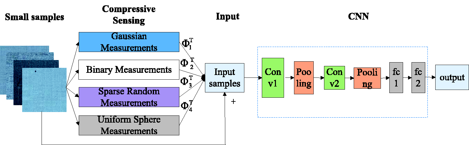

Data preprocessing

When a raw defect image is fed into the neural network directly, the classification performance will be significantly subject to noises and abnormal disturbances. For this reason, the original fabric defect images are preprocessed by the following two steps.

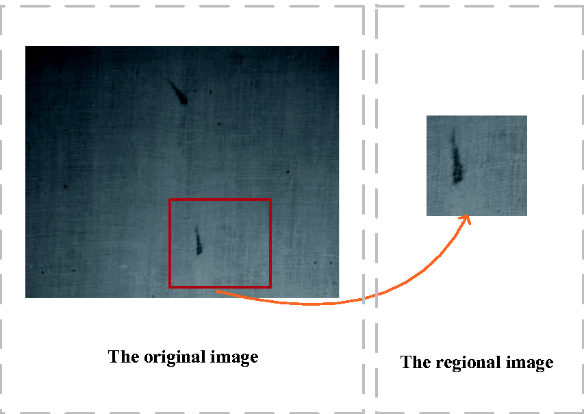
Step 1: segmentation of fabric defects. The original defect images are 1280 × 1024 pixels. It can be seen from Figure 2 that the original images contain noises, which include staining, an irregular texture and a fringe. These noises may be caused by equipment or industrial monitors. The noises can be identified and denoised by filtering, wavelet transform, and so on. In addition, an image may appear on multiple types of different fabric defects. We get the local image blocks of the original images manually that only contain one fabric defect type. The size of the local images is 227 × 227. The preprocessing results of the original images are shown in Figure 3.

Figure 2.

The original fabric defect images.

Figure 3.

The preprocessing result of the original images.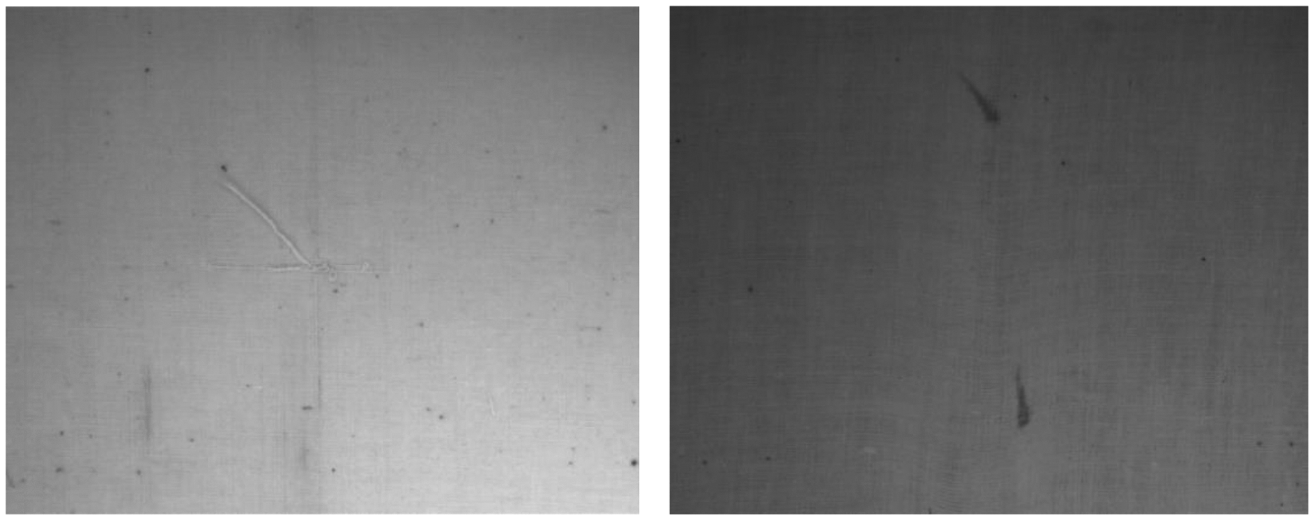

Step 2: diversification of the images. The images are rotated and translated so that the CNNs can learn more invariant image features. The range of rotation is from 5° to 20°, while the range of translation is from 0 to 50 pixels. The results of the image rotation and translation are shown in Figure 4.

Figure 4.

The results of the image rotation and translation.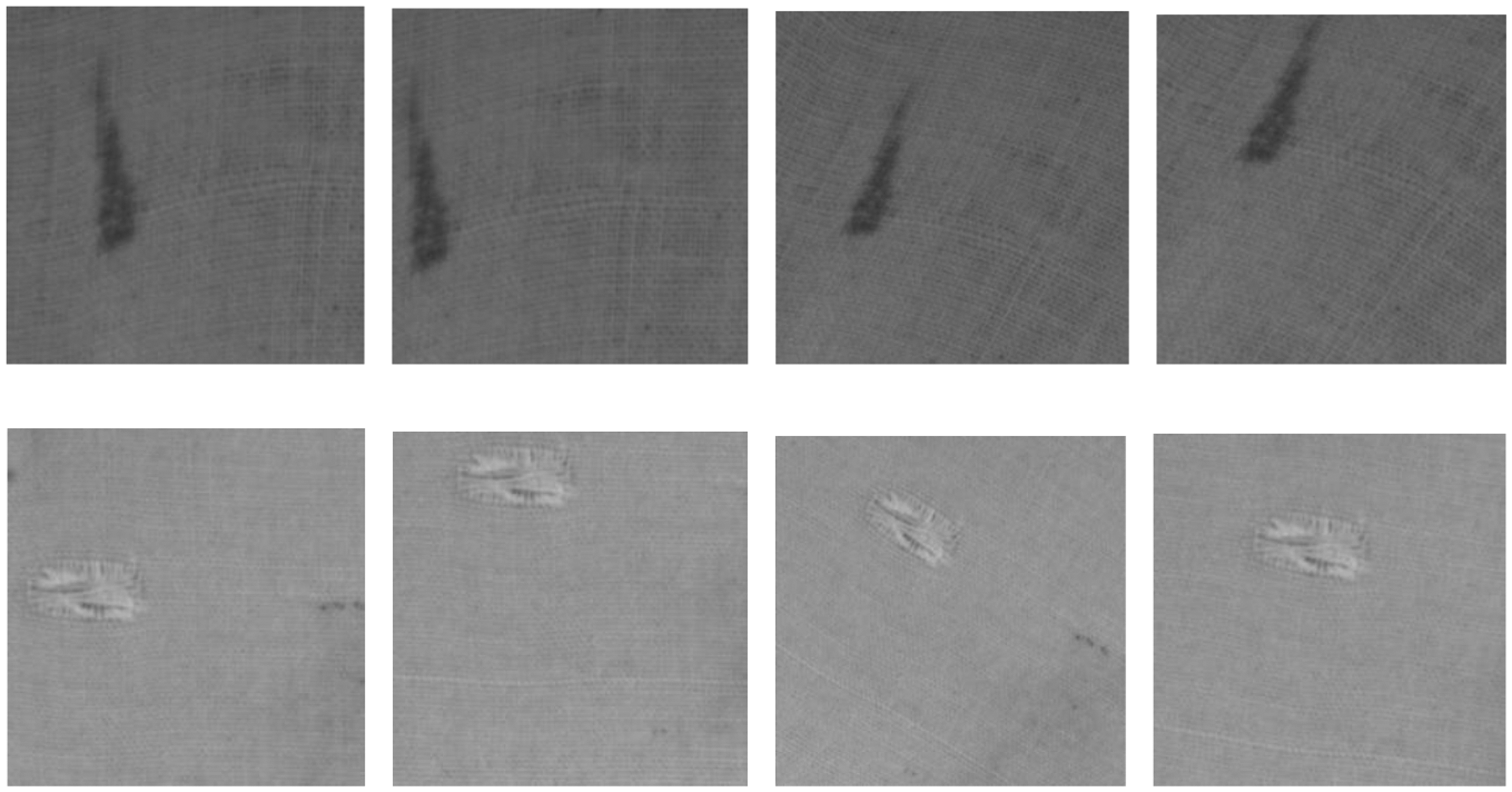

Compressive measurements of defect images

During the data preprocessing, the original defect images are processed to form a small sample dataset. There are 50 of each class image in the small sample dataset. Then, compressive sampling theorem is used to compress and augment the data in small sample sizes. Compressive sensing is mainly used to deal with the one-dimensional vector. The two-dimensional image matrix needs to be converted into a one-dimensional vector. The following steps are carried out.

The fabric defect image $X \in R^{I_{c} \times I_{r}}$ is converted to the one-dimensional vector $x \in R^{N \times 1}$ by formula (8)

x = reshape (X)

(8)

where X is the defect image and R is the real domain,

N = I_{c} \times I_{r}

The Discrete Cosine Transform (DCT) transform formula is used as follows

x = Ψ Θ

(9)

where Θ is the projection coefficient vector and Ψ is the sparse representation matrix,

Ψ \in R^{N \times N}

Based on a variety of different measurement matrices, the observation vector y is given by

y = Φ x = Φ Ψ Θ \overset{=}{Δ} A Θ

(10)

where y is the observation vector of dimension

M \times 1

, while M is the vector length obtained by observing the original signal. Φ is the measurement matrix,

Φ \in R^{M \times N}

A = Φ Ψ

is the compressive sensing matrix.

To obtain the observation vector maps for the image space, the reconstruction accuracy of the construction algorithm is largely influenced by the sampling rate and the noise of compressive observation. In this work, we use a linear mapping method to avoid the design of the reconstruction algorithm

\hat{x} = Φ^{T} y

(11)

where

\hat{x}

is the one-dimensional vector of the observation vector y, which is mapped to the image space.

Φ^{T}

is the transpose matrix of the measurement matrix Φ.

$\hat{x}$ is converted to an image, with the formula given as

X_{out} = reshape (\hat{x})

(12)

where

X_{out}

is the image and

X_{out} \in R^{I_{c} \times I_{r}}

Training the CS-CNN

In the training process of the CNN, the features of input images can be extracted from the previous layer. Then the fully connected layers get the features and make the nonlinear transformation. The output layer is connected to the fully connected layers, which indicates the predicted probability values. The effectiveness of the CNN lies in the local correlation and spatial invariance of the model. It is well known that an image is composed of pixels, which are associated with its surrounding pixels. If we mess up the pixels, the image will be completely changed. The important thing is that the CNN architecture can maintain the local correlation. Meanwhile, a simple CNN structure can extract low-level feature information, such as edges, locations and sizes. As the CNN has a deep network structure, low-level features can be combined to form high-level features, which can keep the spatial invariance of the features. In the proposed CS-CNN, the main structure and parameters of the model are as shown in Table 1. The training process of the CS-CNN is shown in Algorithm 1. Before the training phase, the training data and labels are loaded. The learning rate is set to 0.001. The cross-entropy error⁴⁵ is used as the loss function. The gradient descent method of the model is Adam. Adam is an optimization algorithm that can be used instead of the classical stochastic gradient descent procedure to update network weights iteratively based on training data. The CS-CNN saves a graph of the session during the training phase. The setting of the other parameters in the model is related to the number of samples in the training data and the gradient algorithm in the training phase.

Algorithm 1

Training the CS-CNN model

Table 1.

Structure and parameters of the convolutional neural network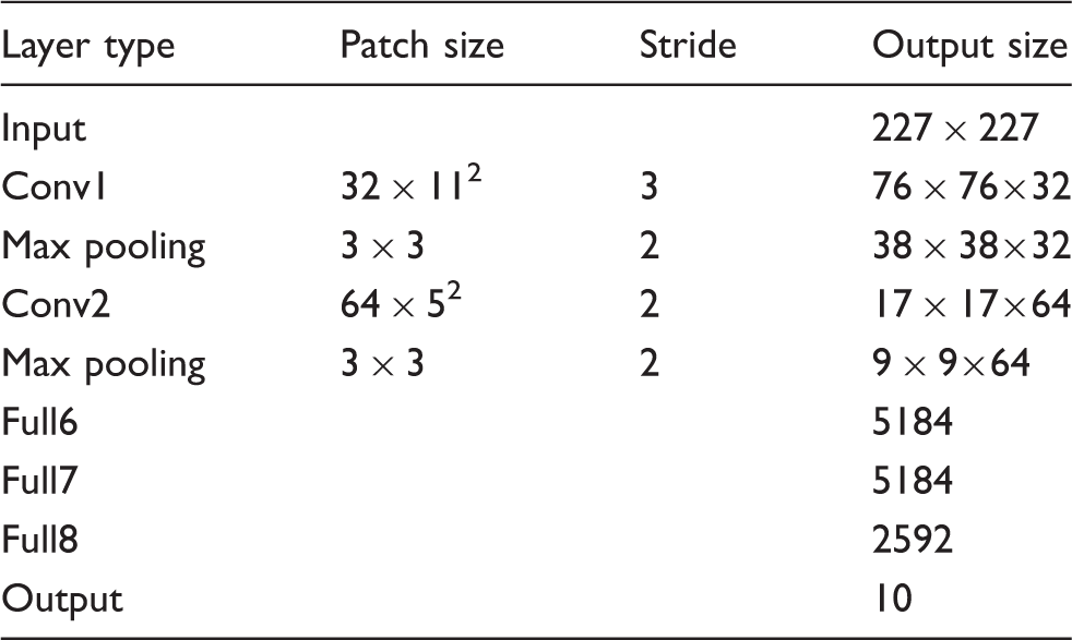

Layer type	Patch size	Stride	Output size
Input			227 × 227
Conv1	32 × 11²	3	76 × 76×32
Max pooling	3 × 3	2	38 × 38×32
Conv2	64 × 5²	2	17 × 17×64
Max pooling	3 × 3	2	9 × 9×64
Full6			5184
Full7			5184
Full8			2592
Output			10

Inputs: The original images and features information; The cross-entropy error is used as the loss function.

Output: Weight and bias matrices; The predicted output of the CS-CNN (labels values)

Procedure:

1: Initialize learning rate, batch size, kernel size, number of kernels, number of max iteration, dropout and so on.

2: Generate random weights with Gaussian type and biases with 0;

CS-CNN_model = InitCS-CNN_model(weights and bias matrices);

3: While iter < max iteration or error > min error do

Compute error according to loss function

For iter = 1 to iter < = number/(batch size) do

CS-CNN_model.train(TrianingData, TraingLabels), as loss is minimalized with gradient descent;

Update weight and bias matrices;

end for

iter ++

end while

4: Save parameters (weight, bias) of the CS-CNN; Save graph of session

5: training CS-CNN Finished

CNN classification recognition

CNNs are special neural network models, which are inspired by the human vision system. On one hand, the connections in the neurons are sparsely connected; on the other hand, the convolution layers of CNNs have shared weights. CNNs can improve the accuracy of detection and classification by studying the spatial correlation of data and reducing the number of training parameters in the network. In this work, a new adaptive expansion is designed based on the basic CNN that is shown in Figure 1. The number and size of convolution kernels have been redesigned by considering the characteristics of fabric defect images. We add one fully connected layer based on the two fully connected layers. The nonlinear ability of the CNN can be enhanced when adding one fully connected operation. The structure of a CNN is represented in Figure 5. The output is identified as a certain type, which is the mispick in Figure 5.

Figure 5.

The structure of a convolutional neural network (CNN). The input image uses the fabric defect “mispick” as an example.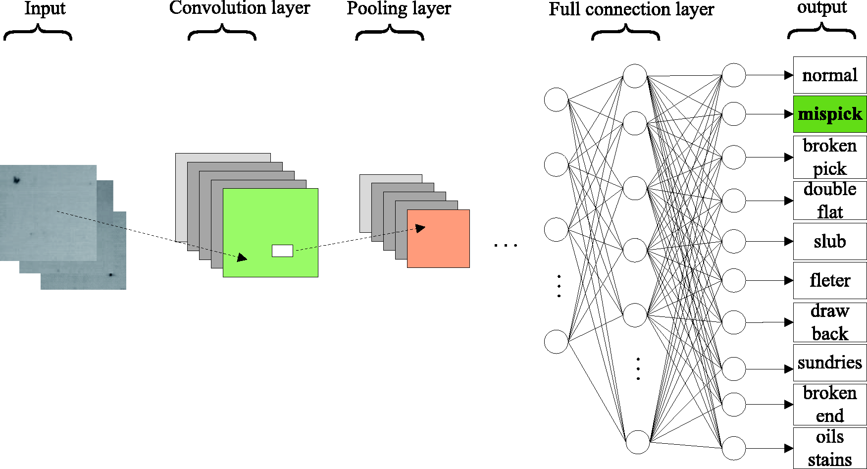

Experimental evaluations and discussion

In order to evaluate the CS-CNN classification performance in fabric defect images, many experiments were completed to compare with KNN, multi-layer perceptron (MLP) and SVM.

The fabric defect images dataset (FDI 500)

Our experimental images are acquired using industrial monitors from a textile factory. The fabric defect dataset is built by ourselves. The original defect images are cut, rotated and translated to form a small sample dataset. Ten different fabric defect classes of the original images were selected, which included one normal fabric sample and nine different defect samples. The flaw samples are normal, mispick, broken pick, double flat, slub, felter, draw-back, sundries, broken end and oil stains, which are shown in Figure 6. There are 50 images of each class in the small sample dataset. Each measurement matrix can generate 500 images. The four measurement matrices can generate 2000 images. Namely, the dataset, which contains 2500 images through compressive sampling by different measurement matrices, is divided into train, validation and test subsets. In this work, 80% (2000) of the images are used as the training samples and 10% (250) of the images are used as the validation samples; the remaining samples (250) are used for prediction.

Figure 6.

Normal and defect images (normal, mispick, broken pick, double flat, slub, felter, draw-back, sundries, broken end and oil stains).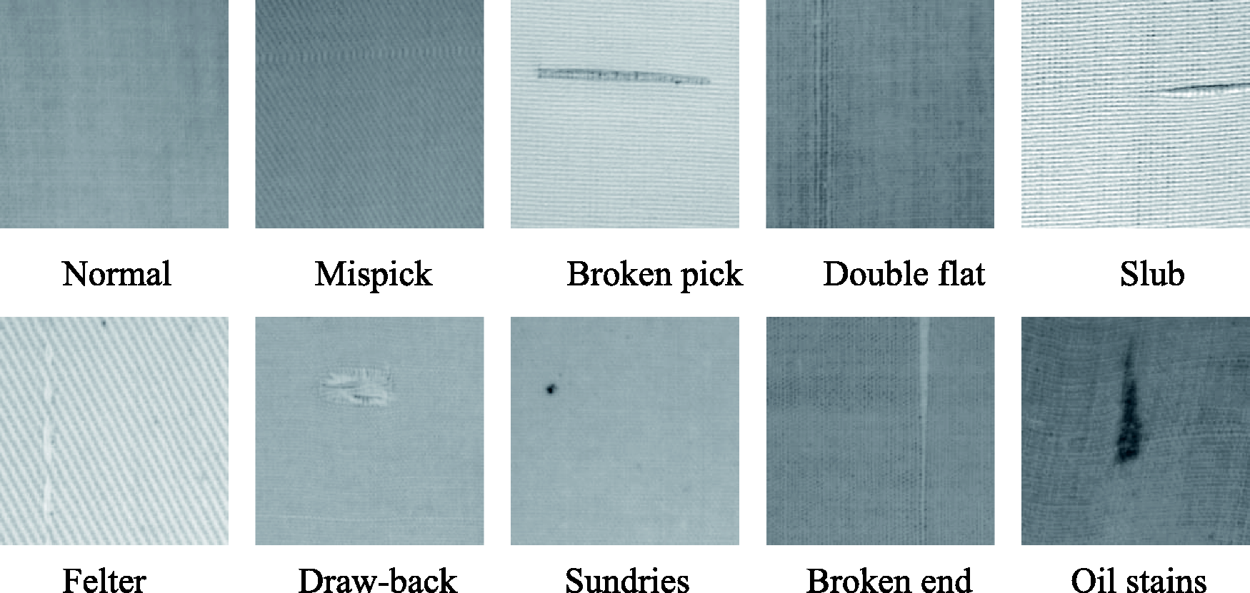

Environmental configurations

The experiments were implemented on a PC with four Nvidia GeForce GTX 1080 GPUs, 128GB RAM. The operation system was on an Ubuntu 14.04 with tensorflow 0.8.0. The proposed algorithm is performed on the software of MATLAB and PYTHON. The most critical factor in fabric defect classification is the classification accuracy and speed. The average classification speed is less than 1 second on the platform, which can satisfy the general requirements of online defect classification. We evaluate the performance of the method with classification accuracy.

Feature information of defect images with different measurement matrices

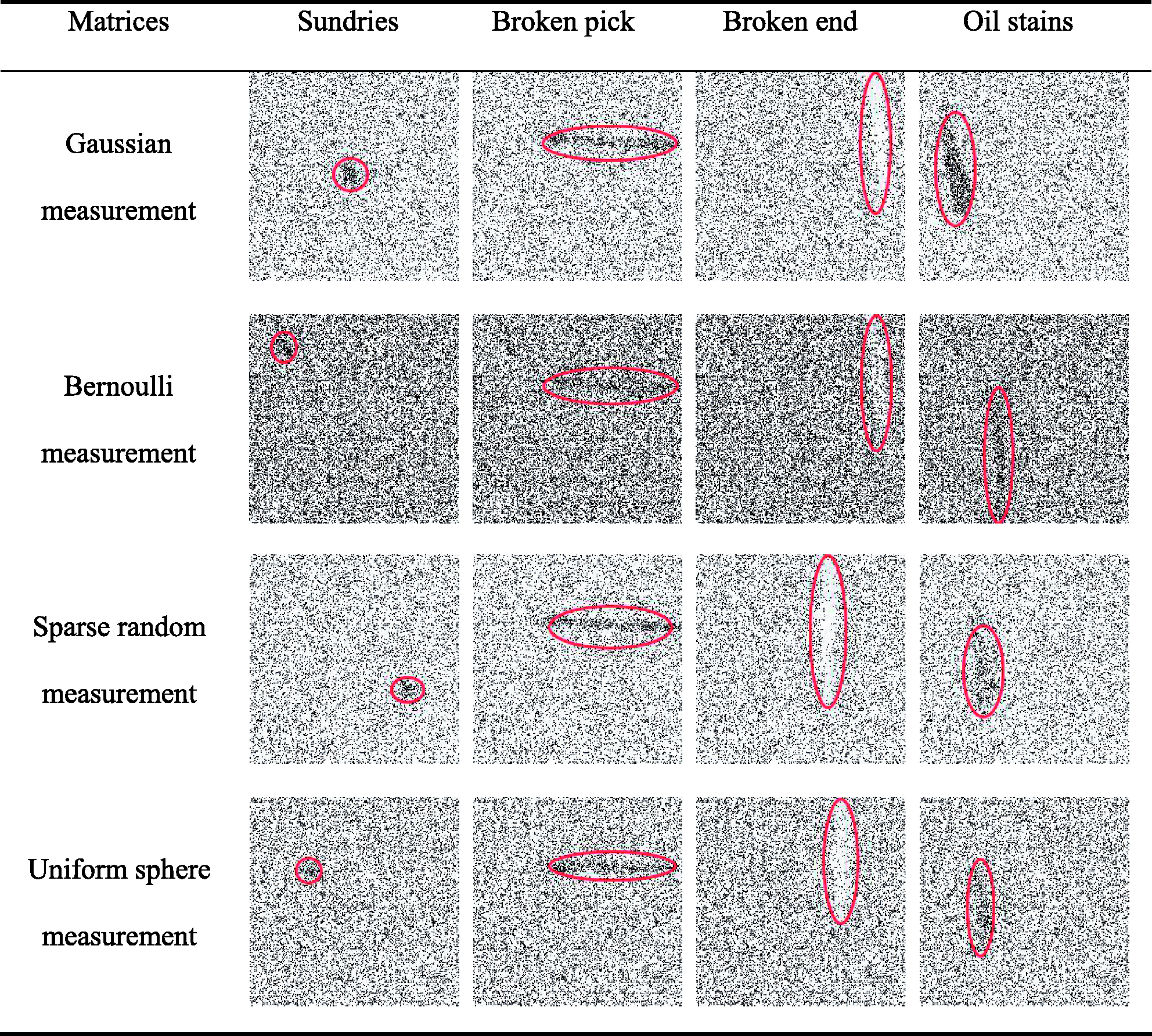
A variety of different measurement matrices are tested to extract feature information, such as Gaussian measurement matrices,⁴⁴ Fourier measurement matrices,⁴⁴ Bernoulli measurement matrices,⁴⁶ random sparse measurement matrices,⁴⁷ uniform sphere measurement matrices,²³ Toeplitz measurement matrices⁴⁸ and Hadamard measurement matrices.⁴⁹ We find that some measurement matrices cannot obtain good feature information. The reasons can be summarized as follows. (1) The measurement matrices do not satisfy the form of the input data, such as Hadamard measurement matrices, where the dimension must satisfy the integral multiple of 2. The size of the input image in this work is 51,529. (2) The measurement matrices, such as Fourier measurement matrices, which require the input image to satisfy the sparsity in the Fourier domain. (3) The linear mapping by formula (11) cannot obtain better feature information to the partial measurement matrices, such as Fourier measurement matrices and Toeplitz measurement matrices. After analyzing the test result and reasons, we finally selected four measurement matrices, which are Gaussian measurement matrices, Bernoulli measurement matrices, random sparse measurement matrices and uniform sphere measurement matrices.

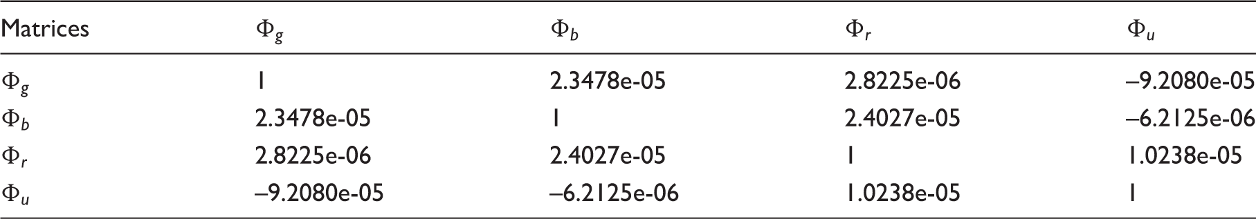
The four different measurement matrices are used to compressive measure x by formula (7). Figure 7 shows the partial feature information of the defect images. We have studied the correlation coefficient of the selected measurement matrices in order to illustrate the differences of the extracted feature information by different measurement matrices. The formula used is as follows

corr = \frac{\sum_{m} \sum_{n} (A_{mn} - \bar{A}) (B_{mn} - \bar{B})}{\sqrt{(\sum_{m} \sum_{n} {(A_{mn} - \bar{A})}^{2}) (\sum_{m} \sum_{n} {(B_{mn} - \bar{B})}^{2})}}

(13)

where A and B are matrices, m is the row of matrices and n is the column of matrices.

\bar{A}

and

\bar{B}

are the mean of the element values of matrices A and B, respectively. The function returns a correlation coefficient between –1 and 1, where –1 or 1 means complete correlation and 0 means completely irrelevant. In Table 2, correlations with the same measurement matrices are 1 and correlations with different measurement matrices are nearly zero, which indicates that the feature information is different.

Figure 7.

Feature information of defect images with the four measurement matrices.

Table 2.

Correlation coefficient with different measurement matrices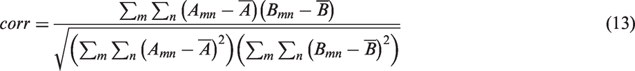

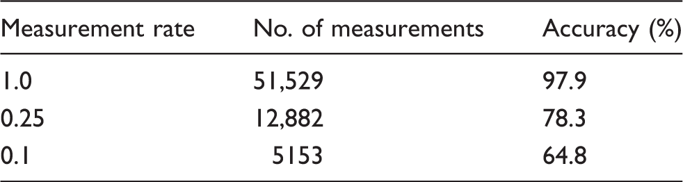
Matrices	$Φ_{g}$	$Φ_{b}$	$Φ_{r}$	$Φ_{u}$
$Φ_{g}$	1	2.3478e-05	2.8225e-06	–9.2080e-05
$Φ_{b}$	2.3478e-05	1	2.4027e-05	–6.2125e-06
$Φ_{r}$	2.8225e-06	2.4027e-05	1	1.0238e-05
$Φ_{u}$	–9.2080e-05	–6.2125e-06	1.0238e-05	1

Comparison of classification accuracy with different sampling rates

In the process of compressive sampling, different sampling rates have an important effect on the results. The networks are trained, with the same architecture, at three different measurement rates of 1.0, 0.25 and 0.1. Since the number of pixels in the reshaped images is 51,529, these measurement rates correspond to 51,529, 12,882 and 5153 pixels, respectively. The classification accuracy on the test set at different measurement rates is shown in Table 3. The accuracy is not so bad compared with the case without compression, which means the CS-CNN still has basic recognition ability with the measurement rate of 0.1.

Table 3.

The classification accuracy at different measurement rates

Measurement rate	No. of measurements	Accuracy (%)
1.0	51,529	97.9
0.25	12,882	78.3
0.1	5153	64.8

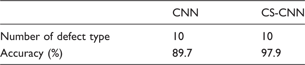
Performance comparison of defect classification models

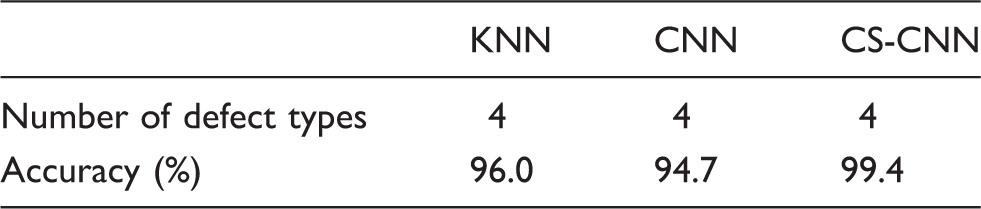
We compare the results of the proposed CS-CNN and a traditional CNN on the fabric defect images. Table 4 shows the details of improvements of the CS-CNN. The classification performance can be further improved by at least 8.2%. In order to further verify the effectiveness of the proposed model for defect classification, its classification performance is compared with the other three existing approaches. Among the three selected methods, the first one is based on a KNN.¹³ The second method selected for comparison utilizes the MLP neural network⁸ combined with the Dempster–Shafer theory. The last method uses combined features and the modified SVM¹² to classify the defect images.

Table 4.

Classification accuracy of the convolutional neural network (CNN) and the compressive sensing and convolutional neural network (CS-CNN)

	CNN	CS-CNN
Number of defect type	10	10
Accuracy (%)	89.7	97.9

Tables 5 and 6 present the classification results of comparison experiments with the same defect type. It can be seen that our CS-CNN can achieve higher accuracy when the number of defect types is the same. This paper also compares the CNN with three existing methods with the same defect type. It can be observed that the CNN performs slightly better than the other three methods. Table 7 shows the results of the five different methods in the case of the CNN and the CS-CNN using 10 classes of defect images. It can be seen from the experimental results that the proposed CS-CNN method outperforms the other four existing methods on this dataset. We can also conclude from Tables 5–7 that the classification performances will be reduced as the number of defect types increases. This could be explained by considering the following two aspects. Firstly, the complexity of the training model will be increased so that the task of classification will be more difficult with more fabric defect types. Secondly, the diversity of fabric defects within one class will also affect the result of classification with more fabric defect images.

Table 5.

Classification accuracy of the k-nearest neighbor algorithm (KNN), convolutional neural network (CNN) and compressive sensing and convolutional neural network (CS-CNN)

	KNN	CNN	CS-CNN
Number of defect types	4	4	4
Accuracy (%)	96.0	94.7	99.4

Table 6.

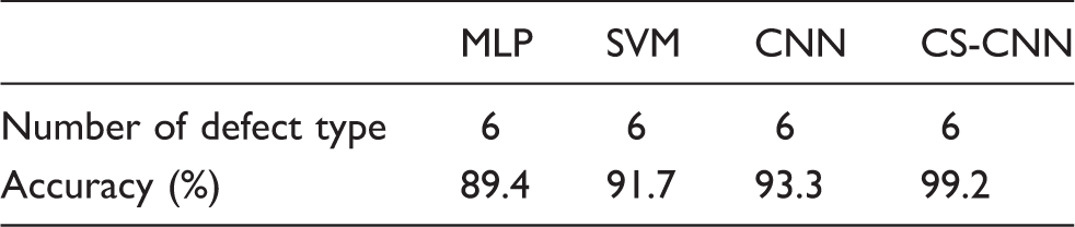
Classification accuracy of the multi-layer perceptron (MLP), support vector machine (SVM), convolutional neural network (CNN) and compressive sensing and convolutional neural network (CS-CNN)

	MLP	SVM	CNN	CS-CNN
Number of defect type	6	6	6	6
Accuracy (%)	89.4	91.7	93.3	99.2

Table 7.

Classification accuracy of five methods

	KNN	MLP	SVM	CNN	CS-CNN
Number of defect type	4	6	6	10	10
Accuracy (%)	96.0	89.4	91.7	89.7	97.9

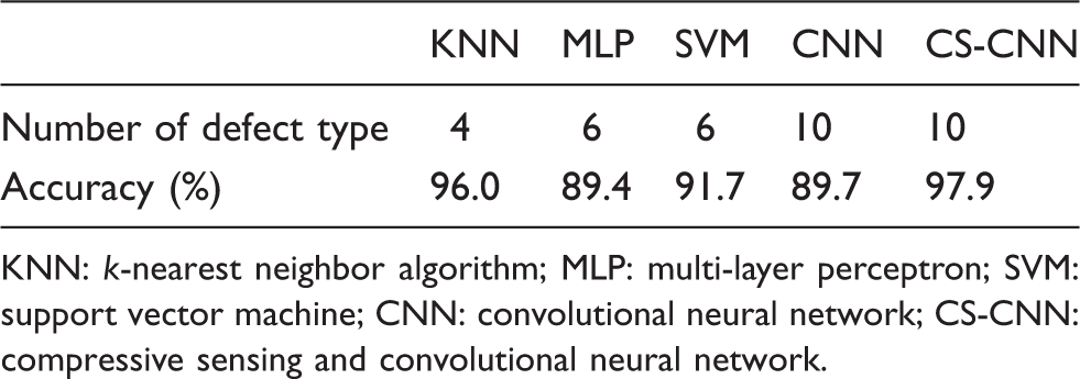
KNN: k-nearest neighbor algorithm; MLP: multi-layer perceptron; SVM: support vector machine; CNN: convolutional neural network; CS-CNN: compressive sensing and convolutional neural network.

Performance comparisons of different parameters

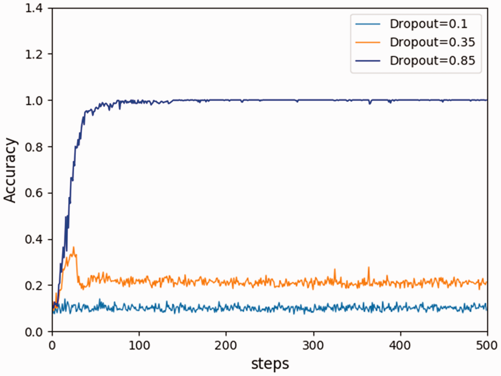
In the experiment, we find that some parameters can affect the performance of the proposed method, such as the learning rate, batch size, training iteration, dropout and convolution kernel. In order to explore the relationship among partial parameters and classification accuracy, in this study the influences of batch size and dropout on the results are analyzed. The number of fabric defect classes is 10. The measurement rate is fixed to 1. The number of training iterations is 500. For each of the parameters, the number of trainings is fixed to 10 times. Figures 8 and 9 show the change of the accuracy obtained by different batch sizes and dropouts. Figure 8 shows that the classification accuracy is not so good with the batch sizes of 128 and 256. The best accuracy is 97.9% with the batch size of 512. Figure 9 shows the results of the accuracy at three different dropouts. When the model is trained with different dropouts, the batch size is 512. It can be seen that the average accuracy reaches 97.9% when the dropout is 0.85. The partial curves have a slight fluctuation in Figures 8 and 9. This phenomenon may be caused by redundant information and different features in each batch of images.

Figure 8.

The result of different batch sizes.

Figure 9.

The result of different dropout rates.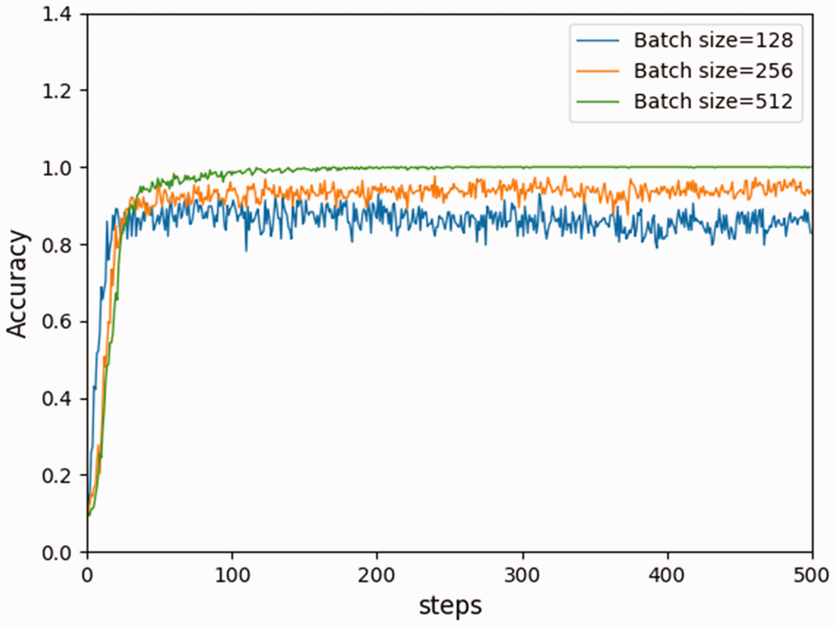

Visualizing partial results

In this research, the CNN model is a complex black-box model, in order to further understand the learning process of the model more intuitively. Meanwhile, we attempt to explain how the network learns the feature and weights when the data is input to the CNN model and some visualization results are given.

Visualization of the convolution layer

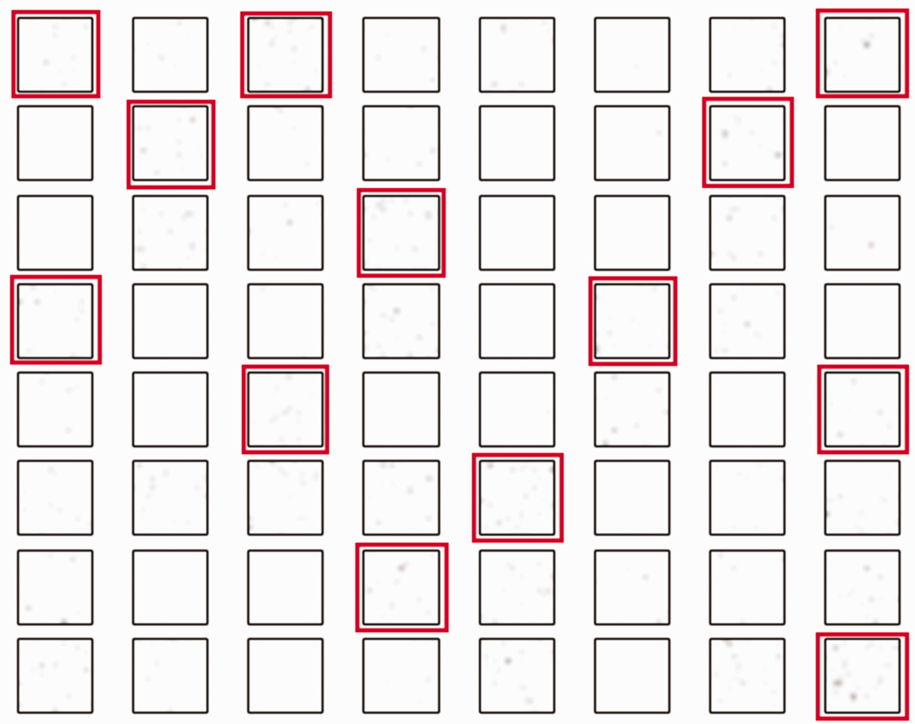
Figures 10 and 11 show the feature map visualization of the convolution layer. It can be seen from the feature map that the first convolution layer can learn some low-level features, such as color, edge and size. The second convolution layer can learn the more discriminative and distinguishing features, such as fabric defect and texture.

Figure 10.

The feature map of convolution layer 1. Each block is a convolution kernel, while the size of each block is 11 × 11. There are 32 different convolution kernels in convolution layer 1.

Figure 11.

The feature map of convolution layer 2. Each block is a convolution kernel, while the size of each block is 5 × 5. There are 64 different convolution kernels in convolution layer 2.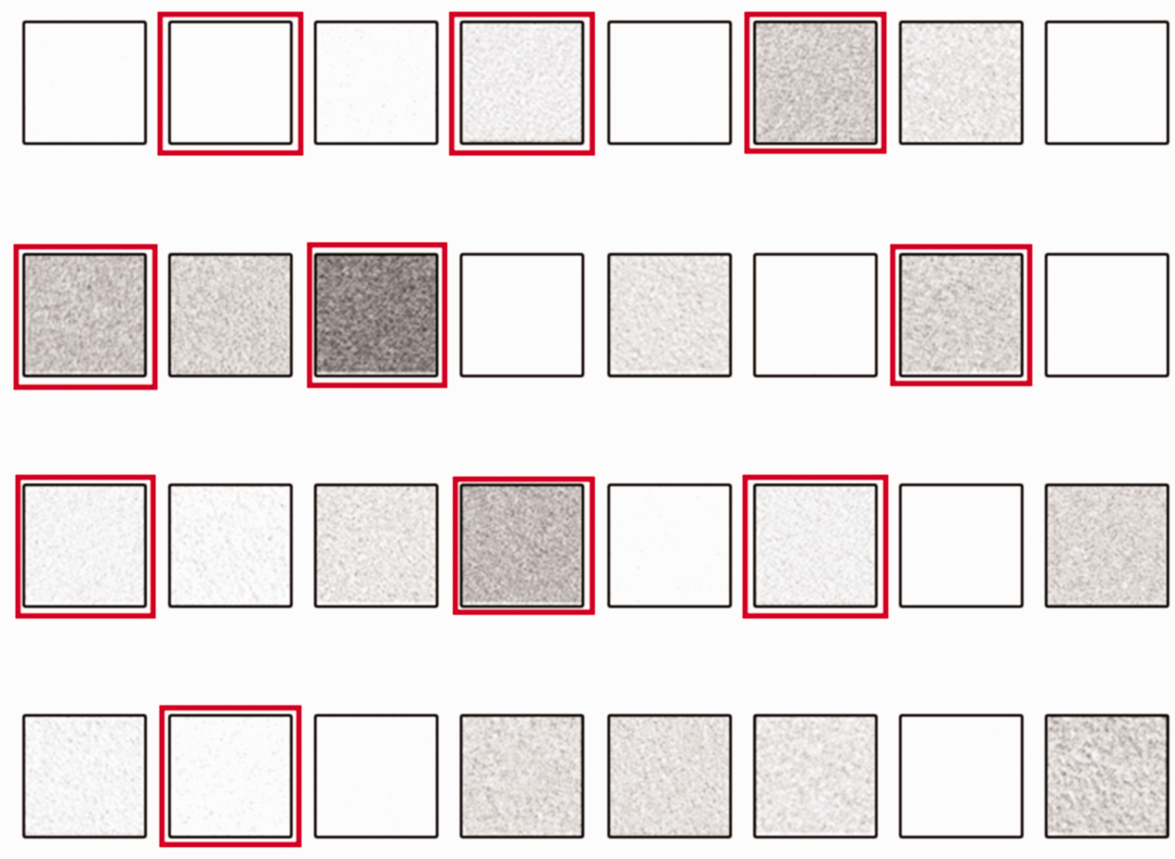

Feature visualizations with different parameters

This work visualizes the results of several layers of the trained model with different parameters to analyze the relationships between the accuracy of classification and the process of training the model.

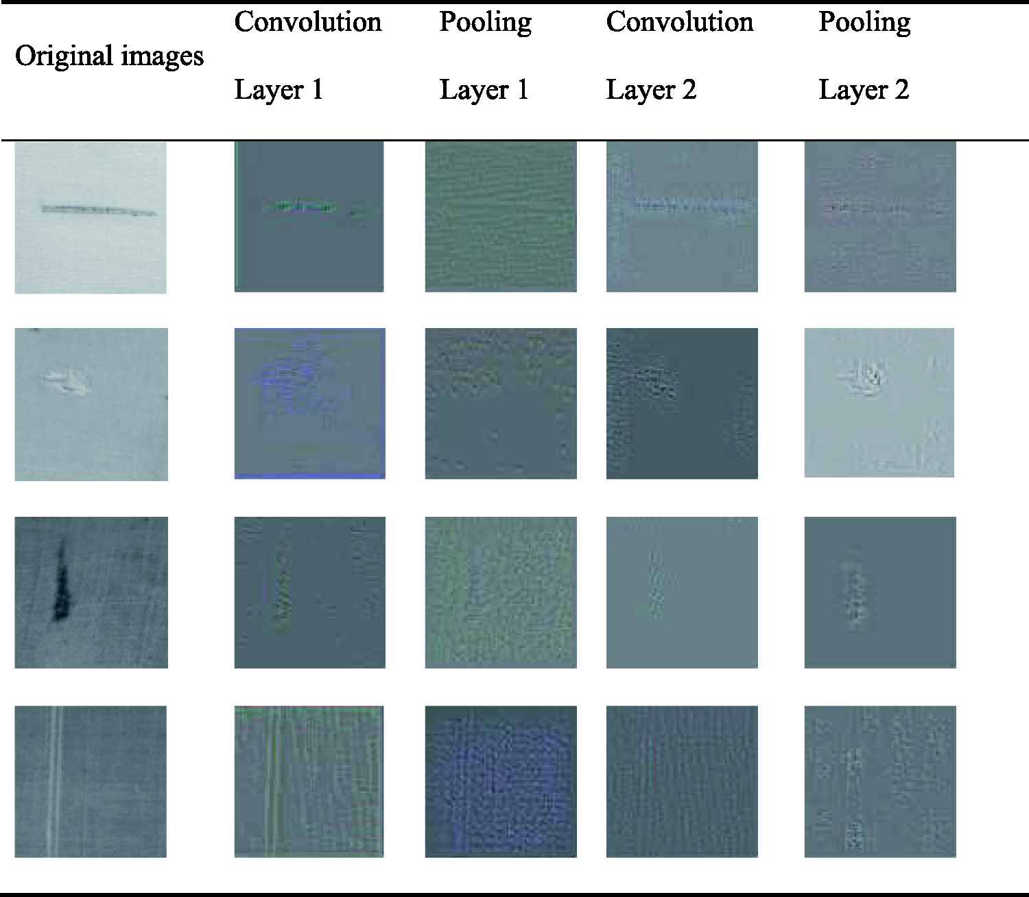
Figures 12 and 13 show the results of convolution layers and pooling layers for which the batch sizes are 64 and 512, respectively. Figure 12 shows that the proposed CS-CNN does not learn the necessary feature information with the batch size of 64. Namely, the important feature information is not clearly expressed in the model, such as the broken pick, draw-back, oil stains and broken end. The CS-CNN cannot achieve a high accuracy of classification with a batch size of 64.

Figure 12.

Visualizations with the batch size of 64.

Figure 13.

Visualizations with the batch size of 512.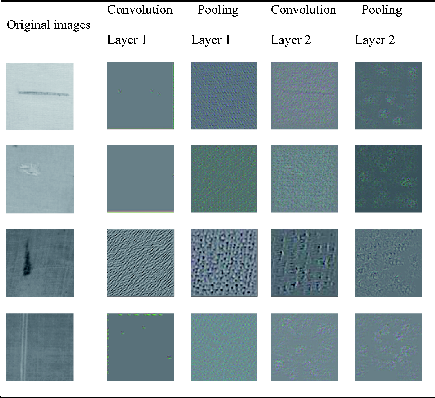

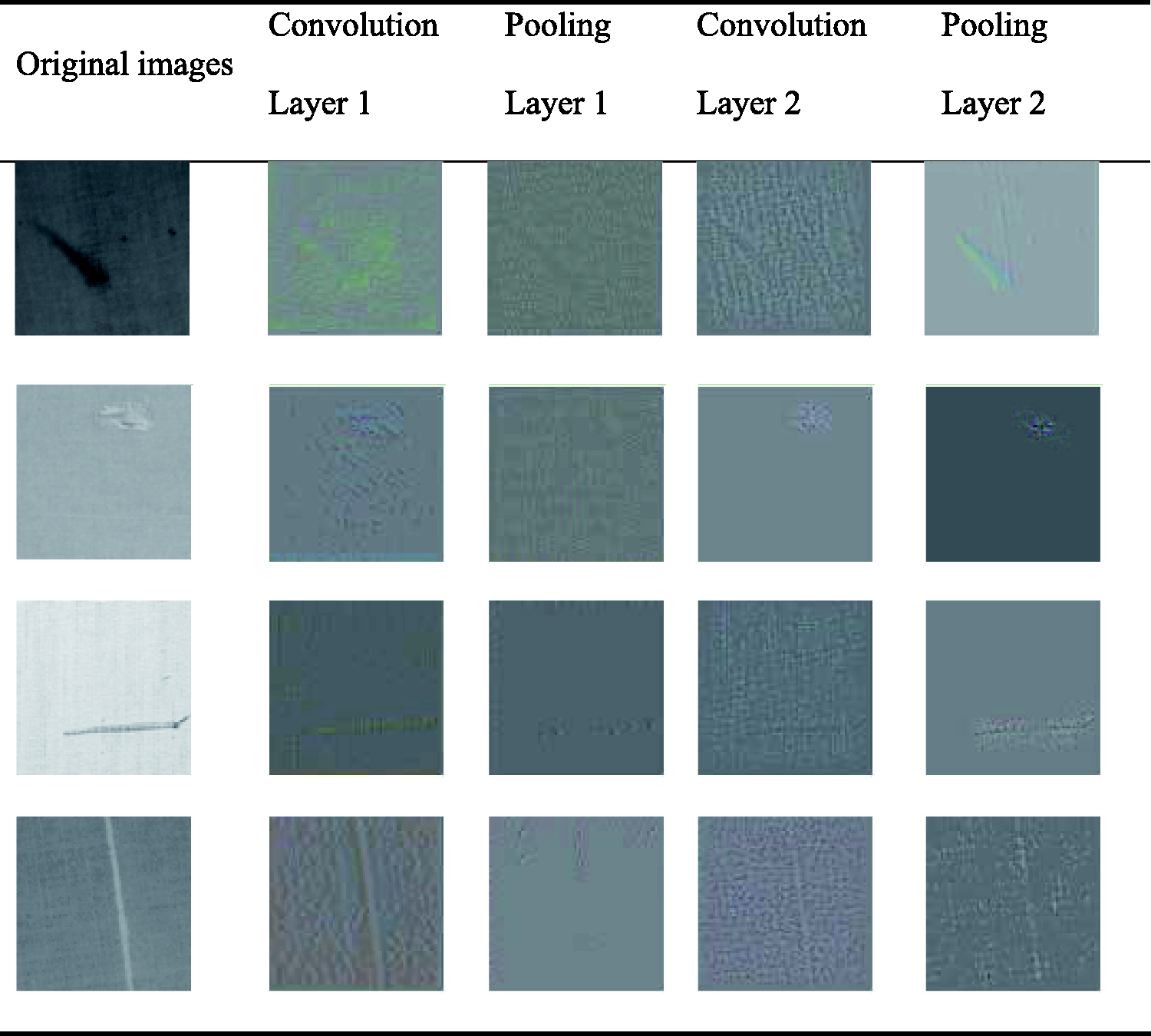
In Figure 13, the important feature information of the defects can be learned obviously with the batch size of 512. With the learned important information, the dependence of the model on the classifier will be reduced and the classification performance of the model can also be improved. Figures 14 and 15 show the results of convolution layers and pooling layers for which the dropouts are 0.1 and 0.85, respectively. In Figure 14, the proposed CS-CNN loses the ability to learn the important feature information of images with the dropout of 0.1. With the extraction of better feature information, the model has a better accuracy of classification with the dropout of 0.85. It can also be observed from Figures 13 and 15 that not all of the feature information can be extracted well, even if the model has a better accuracy of classification, such as images of broken ends.

Figure 14.

Results with a dropout of 0.1.

Figure 15.

Results with a dropout of 0.85.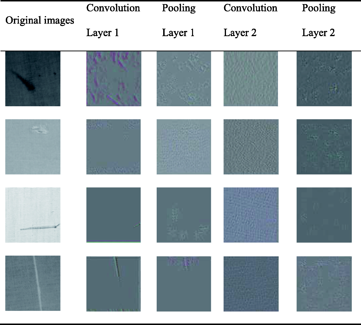

Tracking of weights of the fully connected layer

In the training process, the stability of the weights is also an important basis for considering whether the model can converge to the stable state. In this work, we track the changes of weights in the third fully connected layer. It can be seen from Table 1 that there are 2592 connection weights in the third fully connected layer. The initial weights are randomly generated, so it is not necessary to track all connection weights. We select five weights randomly and track the changes when the model is in the training phase. Figure 16 shows the changing trend when the batch size is 512 and the dropout is 0.85. With the training process of the model, it can be seen that the selected weights tend to be stable finally. It can be concluded that the model can converge to the stable state with stable weights.

Figure 16.

The tracking results of weights.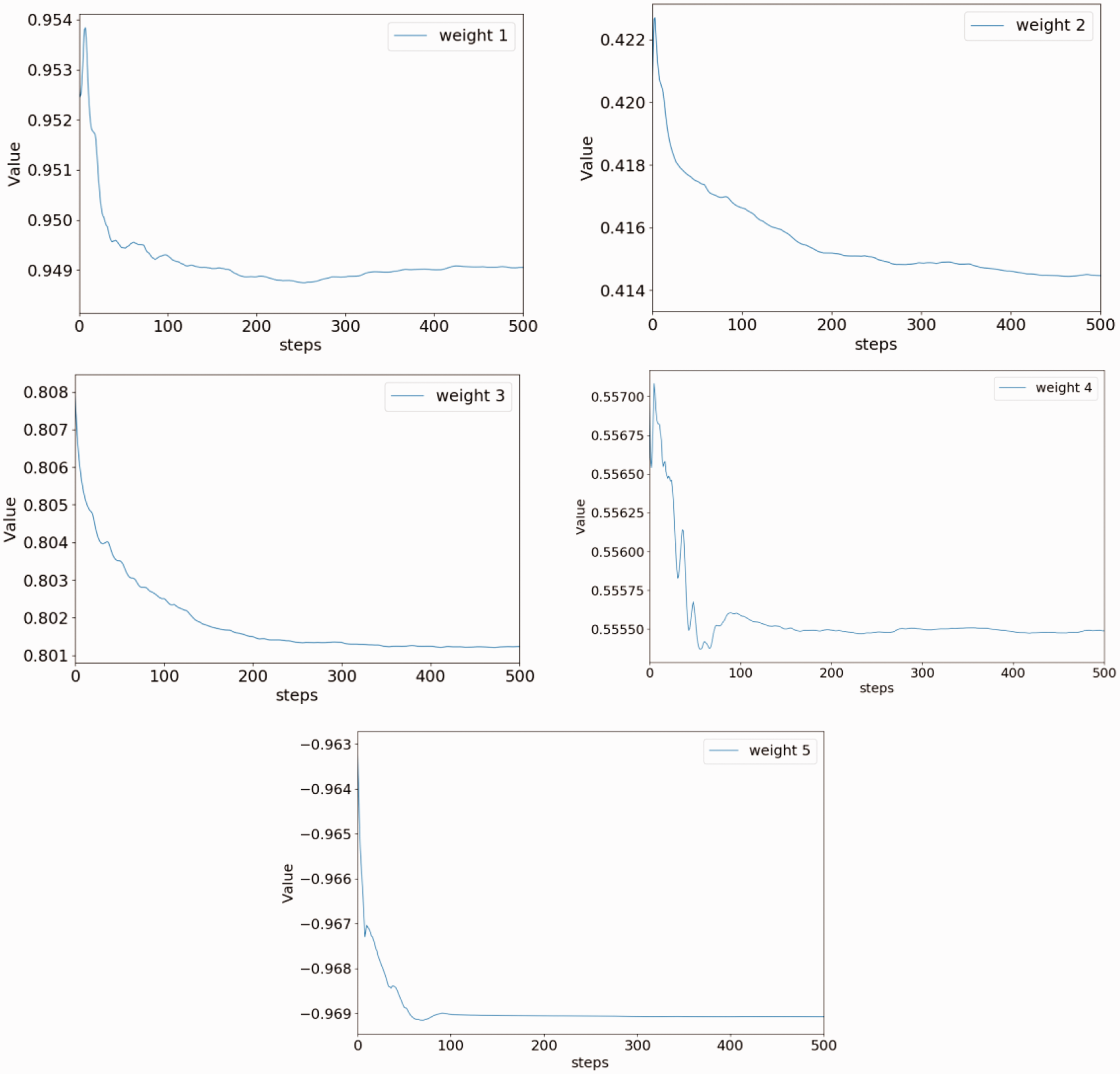

Conclusions and future work

In this research, a novel method CS-CNN is proposed to solve the problem of fabric defect classification in small sample sizes, which is based on CS and CNNs. Different types of feature information are extracted by CS. Utilizing this feature information and the original images, the newly designed CS-CNN model is used to classify the defect images. The experimental results show the effectiveness of the proposed method in comparison with the usual classification techniques, where we observe that even at low measurements rates, excellent classification recognition accuracy can be obtained. Meanwhile, this study visualizes medium results of the proposed CS-CNN that help one to better understand and explain the effects of the model. Further investigation is required to research the unique particularity of the fabric defect images and optimize the architecture in terms of a low measurement rate to maximize the classification performance.

Footnotes

Declaration of conflicting interests

The authors declared no potential conflicts of interest with respect to the research, authorship and/or publication of this article.

Funding

The authors disclosed receipt of the following financial support for the research, authorship, and/or publication of this article: This work was supported in part by the International Collaborative Project of the Shanghai Committee of Science and Technology (Grant No. 16510711100), the Fundamental Research Funds for the Central Universities (Grant No. 2232017D-08, 2232017D-13), the National Natural Science Foundation of China (Grant Nos. 61503075, 61603090), the Shanghai Sailing Program (Grant No. 17YF1426100) and the Program for Changjiang Scholars from the Ministry of Education (2015-2019).

References

Zheng

Han

Jin

. A new method for classification of woven structure for yarns-dyed fabric. Text Res J 2014; 84: 78–95.

Mehta

Egiazarian

. Texture classification using dense micro-block difference. IEEE Trans Image Proc 2016; 25: 1604–1616.

Boulkenafet

Komulainen

Hadid

. Face spoofing detection using colour texture analysis. IEEE Trans Inform Forens Secur 2016; 11: 1818–1830.

Allili

Baaziz

Mejri

. Texture modeling using contourlets and finite mixtures of generalized Gaussian distributions and applications. IEEE Trans Multimedia 2014; 16: 772–784.

Shady

Gowayed

Abouiiana

. Detection and classification of defects in knitted fabric structures. Text Res J 2006; 76: 295–300.

Connor

Bryan

Nolan

. Modeling Australian land use competition and ecosystem services with food price feedbacks at high spatial resolution. Environ Model Software 2015; 69: 141–154.

Xin

Zhang

. Color texture classification of yarn-dyed woven fabric based on dual-side scanning and co-occurrence matrix. Text Res J 2017; 87: 1883–1895.

Tabassian

Ghaderi

Ebrahimpour

. Knitted fabric defect classification for uncertain labels based on Dempster-Shafer theory of evidence. Expert Syst Appl 2011; 38: 5259–5267.

Zhang Y, Lu Z and Li J. Fabric defect detection and classification using Gabor filters and Gaussian mixture model. In: Hongbin Z, Rin-ichiro T and Stephen M (eds) 9th Asian conference on computer vision, Xi’an, China, 23–27 September 2009, pp.635–644. Berlin, Heidelberg: Springer.

10.

Tong

Wong

Kwong

. Differential evolution-based optimal Gabor filter model for fabric inspection. Neurocomputing 2016; 173: 1386–1401.

11.

Ding

. Characterization and assessment of fabric smoothness appearance based on sparse coding. Text Res J 2018; 88: 367–378.

12.

Cheng

. Yarn-dyed woven defect characterization and classification using combined features and support vector machine. J Text Inst 2014; 105: 163–174.

13.

Yildiz

Demetgul

. A thermal-based defect classification method in textile fabrics with K-nearest neighbor algorithm. J Ind Text 2016; 45: 780–795.

14.

Kuo

Juang

. A study on the recognition and classification of embroidered textile defects in manufacturing. Text Res J 2016; 86: 207–212.

15.

Chen

Liao

HYM

. A new LDA-based face recognition system which can solve the small sample size problem. Pattern Recognit 2000; 33: 1713–1726.

16.

Maryam

Hassan

. Band clustering-based feature extraction for classification of hyperspectral images using limited training samples. IEEE Geosci Remote Sens Lett 2014; 11: 1325–1329.

17.

Maryam

Hassan

. Feature extraction using attraction points for classification of hyperspectral images in a small sample size situation. IEEE Geosci Remote Sens Lett 2014; 11: 1986–1990.

18.

Zhang

Song

Cui

, et al. Topological analysis and Gaussian decision tree: Effective representation and classification of biosignals of small sample size. IEEE Trans Biomed Eng 2017; 64: 2288–2299.

19.

Shu

Zheng

. Classifier-designing algorithm on a small dataset based on margin fisher criterion and transfer learning. Acta Automatica Sinica 2016; 42: 1313–1321.

20.

Zhang

. A nonlinear multiple feature learning classifier for hyperspectral images with limited training samples. IEEE J Select Topic Appl Earth Observ Remote Sens 2015; 8: 2728–2738.

21.

Hamidullah

Gokhan

Semih

. Kernel Fukunaga-Koontz transform subspaces for classification of hyperspectral images with small sizes. IEEE Geosci Remote Sens Lett 2015; 12: 1287–1291.

22.

Aydemir

Bilgin

. Semisupervised hyperspectral image classification using small sample sizes. IEEE Geosci Remote Sens Lett 2017; 14: 621–625.

23.

Donoho

. Compressed sensing. IEEE Trans Inform Theor 2006; 52: 1289–1306.

24.

Chen

CLZ

Qin

, et al. Real-time and robust object tracking in video via low-rank coherency analysis in feature space. Pattern Recognit 2015; 48: 2885–2905.

25.

Jia

Gao

Guo

. Fast compressive tracking with robust example selection based on multiple instance learning in smart and autonomous systems. Pattern Recognit 2017; 69: 336–351.

26.

Lorenzo

Giacomo

Federico

, et al. MT-BCS-based microwave imaging approach through minimum-norm current expansion. IEEE Trans Antenna Propagat 2013; 61: 4722–4732.

27.

Giulio

Simeon

Andrea

, et al. Progressive compressed sensing and reconstruction of multidimensional signals using hybrid transform/prediction sparsity model. IEEE J Emerg Select Topic Circ Syst 2012; 2: 340–352.

28.

Mehta

Majumdar

. RODEO: Robust DE-aliasing autoencoder for real time medical image reconstruction. Pattern Recognit 2017; 63: 499–510.

29.

Niranjan

Arun

. Interferer identification in HerNets using compressive sensing framework. IEEE Trans Commun 2013; 61: 4780–4787.

30.

Wang

Zhang

. Magnetic resonance fingerprinting with compressed sensing and distance metric learning. Neurocomputing 2016; 174: 560–570.

31.

Stolkin

Jiao

, et al. A compressed sensing approach for efficient ensemble learning. Pattern Recognit 2014; 47: 3451–3465.

32.

Xie

. Hyperspectral image reconstruction by deep convolutional neural network for classification. Pattern Recognit 2017; 63: 371–383.

33.

Wei

Xia

Lin

, et al. HCP: A flexible CNN framework for multi-label image classification. IEEE Trans Pattern Anal Mach Intell 2016; 38: 1091–1097.

34.

Yu YC, Hao KR and Ding YS. A new image classification model based on brain parallel interaction mechanism. Neurocomputing. 2018; 315: 190–197.

35.

Xie

Zhang

Yan

, et al. Hybrid CNN and dictionary-based models for scene recognition and domain adaption. IEEE Trans Circ Syst Video Technol 2017; 27: 1263–1274.

36.

Xie

Shi

, et al. Multilevel cloud detection in remote sensing images based on deep learning. IEEE J Select Topic Appl Earth Observ Remote Sens 2017; 10: 3631–3640.

37.

Cao

Zhang

Wen

. Fabric defect inspection using prior knowledge guided least squares regression. Multimedia Tool Appl 2017; 76: 4141–4157.

38.

Jing

Dong

. Yarn-dyed fabric defect classification based on convolutional neural network. Opt Eng 2017; 56: 1–9.

39.

Wang XX, Chen Z, Liu GH, et al. Fiber image classification using convolutional neural networks. In: 4th international conference on systems and informatics, Hangzhou, China, 11–13 November 2017, pp.11–13. IEEE.

40.

Zhang

Lin

. Combining fisher criterion and deep learning for patterned fabric defect inspection. IEICE Trans Informat Syst 2016; E99D: 2840–2842.

41.

Zhao

Pan

. Deformable patterned fabric defect detection with fisher criterion-based deep learning. IEEE Trans Automat Sci Eng 2017; 14: 1256–1264.

42.

Mei

Wang

Wen

. Automatic fabric defect detection with a multi-scale convolutional denoising autoencoder network model. Sensors 2018; 18: 1–18.

43.

Richard

Emmanuel

Robert

. Compressive sampling. IEEE Signal Proc Mag 2008; 25: 12–13.

44.

Candes

. Compressive sampling. Marta Sanz Sole 2007; 17: 1433–1452.

45.

Cheng

Yang

Yao

, et al. When deep learning meets metric learning: remote sensing image scene classification via learning discriminative CNNs. IEEE Trans Geosci Remote Sensing 2018; 56: 2811–2821.

46.

Rauhut

Schnass

Vandergheynst

. Compressed sensing and redundant dictionaries. IEEE Trans Inform Theor 2008; 54: 2210–2219.

47.

Wu K and Guo X. Compressive sensing with sparse measurement matrices. In: proceedings of the 73rd IEEE vehicular technology conference, Yokohama, Japan, 15–18 May 2011, pp.1–5. IEEE.

48.

Tsaig

Donoho

. Extensions of compressed sensing. Signal Proc 2006; 86: 549–571.

49.

Zhao

. Deterministic of real-valued ternary sensing matrices using optical orthogonal codes. IEEE Signal Proc Lett 2013; 20: 1106–1109.