Velocity and pressure visualization of three-dimensional flow in porous textiles

Abstract

Advances in flow visualization techniques based on optics, such as lasers and digital cameras, have contributed considerably to the development of various flow models. However, the uses of optical techniques for flow visualization in porous media are limited owing to the complexity or opaqueness of the medium. This study demonstrates the utilization of magnetic resonance velocimetry to visualize a flow field in a textile material. By using phase-contrast magnetic resonance imaging, a three-dimensional, three-component velocity vector field was obtained for induced flow through a cut-pile carpet owing to the suction of a vacuum cleaner nozzle. As a result, we were able to experimentally identify the flow-dominant region in the carpet. Specifically, velocity vector plots and flow streamlines facilitated the identification of the flow paths, and indicated that the flow was strongest beneath the narrow walls of the vacuum nozzle. In addition, the pressure field in the carpet was estimated by an omni-directional integral method based on the utilization of the visualized velocity field, which showed where the pressure loss was maximized.

Keywords

flow visualization magnetic resonance velocimetry product design management of systems product and systems engineering measurement materials structure-properties pressure visualization

Porous media are utilized in a wide variety of applications, including chemical reactors, underground reservoirs, filters, and textile materials. Fluid flows are often utilized in these applications and, thus, the understanding of relevant transport phenomena, such as heat transfer, diffusion, and dispersion related to the flow, is essential. A flow visualization technique can provide flow information for the porous media aiming toward the development of a flow model, or to the validation of a numerical simulation. However, owing to the structural complexity and opaqueness of the porous material, the application of a flow visualization method is challenging. Instead, numerical simulations based on simple models have been frequently adopted to discover the flow characteristics of porous media.^1–3

Despite the existing difficulties, recent advances in flow visualization techniques have enabled flow measurements in a few porous media types. The flow visualization techniques could be classified into optical and nonoptical techniques. Optical techniques, such as laser Doppler velocimetry (LDV),⁴ particle tracking velocimetry (PTV),^5–9 and particle image velocimetry (PIV),^9–18 have been applied to fundamental types of porous, media such as systems of cylindrical rods^{4,10,14–16,18} and packed beds of spherical particles.^{5–9,11–13,17} However, optical techniques require (a) a flow system that includes transparent fluids and solids to allow the penetration of light and (b) closely matched refractive indices to obtain an undistorted optical flow image. In contrast, these requirements do not apply for nonoptical techniques. Correspondingly, flow visualizations of realistic porous media have received increased attention recently. For instance, X-ray¹⁹ and positron emission tomography²⁰ have been utilized to study flow in sand sediments.

In addition, magnetic resonance velocimetry (MRV) is a versatile, nonoptical flow visualization technique using a magnetic resonance imaging (MRI) scanner. It measures electromagnetic signals emitted from moving atomic nuclei, mostly from the hydrogen protons ¹H in water molecules, in which the spatial and velocity information is encoded by using radio frequency (RF) pulses, an external static magnetic field, and magnetic field gradients. It is capable of quantifying three-component (3C) velocity vectors in a three-dimensional (3D) spatial domain and of measuring the flow in a porous medium even when its pore size is smaller than the imaging voxel. These MRV features have allowed the experimental investigation of flows in various porous media, such as rock cores,^21–24 bones,²⁵ scaled metal foam replicas,²⁶ and bead packs.^{21,24,27–29} Interestingly, instead of velocity measurements, a few studies have measured the distributions of fluid concentrations in carpets,^30–33 papers,³⁴ and fabrics^34,35 by using MRI. However, to date, no studies have reported velocity field measurements in a textile material with MRV, despite its versatile features. In addition, to the best of the authors' knowledge, the estimation of pressure field in a porous medium based on 3D velocity data has rarely been reported.

The main purpose of this study is to demonstrate the applicability of MRV and the omni-directional integration (ODI) method to experimentally visualize 3C velocity and pressure fields in a 3D porous textile material. The details of MRV and ODI are described herein, including their underlying principles and relevant procedures, in conjunction with their measurement accuracies. Another practical purpose is to provide experimental flow data that is useful for engineers to improve the suction nozzle design of a vacuum cleaner. As a textile material, we selected a carpet designated by the International Electrotechnical Commission for a standardized vacuum cleaner performance evaluation (IEC TS 62885–1:2016) to achieve a good practical transferability of the resulting data. Therefore, the characteristics of the flow under a vacuum nozzle are discussed in detail in accordance with the visualization results.

Experimental methods

Phase-contrast MRI

The MRV employed in the present study is a gradient echo-based phase-contrast (PC) MRI technique, commonly known as PC-MRI, which is available in most MRI scanners. It is primarily utilized by clinicians to obtain a velocity field in a cardiovascular system³⁵ and by engineers in laminar or turbulent flow systems.³⁶ Prior to the detailed experimental method, we begin with brief descriptions on the fundamental principle of PC-MRI. More detailed descriptions on the principle and underlying physics may be found in the textbooks written by Haacke et al.³⁷ and Liang and Lauterbaur.³⁸

MRI acquires the MR signal emitted from the proton nuclei in a fluid that is excited with an external magnetic field. These nuclei are called spins because they have nonzero spin values. The spins generate a measurable MR signal by a resonance excitation caused by applying a RF pulse at the Larmor frequency in the presence of a uniform, external, static magnetic field. A spatially varying magnetic field is then generated by using gradient coils that generate magnetic field gradients to encode spatial information to the signal. The MR signals are obtained in a spatial frequency domain referred to as the k-space (Equation (1)). A spatial image (Equation (2)) is obtained by applying the inverse Fourier transform to the k-space signal map

s (k) = \int ρ_{e} (r) e^{- i {2 π k \cdot r + φ (r)}} d 1 r

(1)

ρ_{e} (r) e^{- i φ (r)} = \int s (k) e^{i 2 π k \cdot r} d 1 k

(2)

where

r

indicates the position vector,

ρ_{e} (r)

indicates the spatial distribution of the effective spin density, and

k

denotes the spatial frequency vector. Note that Equation (1) indicates the signal after a demodulation process that eliminated the contribution of the static magnetic field on the phase and that the k-space signals and reconstructed spatial images are complex numbers consisting of magnitude and phase. The spatial frequency is defined by applying magnetic field gradients for a finite duration and expressed as

k (t) = γ \int_{0}^{t} G (t^{*}) d t^{*}

(3)

where

G

denotes the magnetic field gradient vector, which typically has the unit of milli-Tesla per meter, t denotes the time of gradient application, and γ is the gyromagnetic ratio of the spin, which has a unit of MHz per Tesla. Commonly, there are two ways of applying gradients to obtain a different spatial frequency signal in a 3D k-space. One is called a phase encoding gradient and the other is called a frequency encoding gradient, and they are mutually orthogonal. The former is used to generate a constant frequency shift to the signal prior to acquisition by applying a short burst of gradient pulse, and the latter is used to generate a continuously varying frequency by activating a gradient during signal acquisition.

PC-MRI obtains the velocity of moving nuclei from the phase image, $φ (r)$ , as the name implies. It encodes the velocity of moving nuclei to the signal phase. Upon the application of a bipolar magnetic field gradient pulse after a RF excitation pulse, the signal phase accumulates as

φ (r) = φ_{0} (r) + 2 π γ \int_{0}^{τ} G b (t) \cdot r (t) d t

(4)

where

φ_{0} (r)

indicates the initial phase shift and τ is the duration of the bipolar gradient pulse,

G_{b} (t)

. Since the spin is moving, the position vector can be expanded as

r (t) = r_{0} + u_{0} t + \dots

(5)

where

u_{0}

is the velocity vector of spin. Note that an acceleration and higher order terms are ignored. Inserting Equation (5) into Equation (4) gives

\begin{matrix} φ (r) = φ_{0} (r) + r_{0} \cdot 2 π γ {\int_{0}^{τ} G_{b} (t) d t} \\ + u_{0} (r) \cdot 2 π γ {\int_{0}^{τ} t G_{b} (t) d t} \end{matrix}

(6)

where the second term on the right-hand side of Equation (6) is zero because it is the time integration of a bipolar pulse. Thus, the phase after the bipolar gradient consists of

φ_{0} (r)

and the phase proportional to the velocity, and it is simply expressed as

φ (r) = φ_{0} (r) + u_{0} (r) \cdot 2 π γ M_{1}

(7)

where

M_{1}

is the first-order gradient moment, where a gradient moment is defined as

M_{i} = \int_{0}^{τ} t^{i} G_{b} (t) d t

. To eliminate

φ_{0} (r)

, two phase images are obtained with different first-order gradient moments and subtracted. As a result, the phase difference

Δ φ

only depends on the velocity of the moving spins. For example, if two phase images are obtained with and without the bipolar pulse along the x-axis, the resulting phase difference image can be described as

Δ φ (r) = 2 π γ M_{1} u x (r)

(8)

Accordingly, the velocity component in the x-direction, $u_{x} (r)$ , can be obtained as

u_{x} (r) = \frac{VENC}{π} Δ φ (r)

(9)

where VENC is referred to as the encoding velocity defined by the first moment of the gradient pulse and has units of velocity.

For measuring all three velocity components, it requires three phase difference images obtained with three pairs of bipolar gradient pulses with different first moments along each orthogonal direction. There are three methods in general for the acquisition of three phase difference images, which are named the six-point, four-point, and balanced four-point methods.³⁹ As the names suggest, the six-point method independently acquires three phase image pairs, the simple four-point method acquires a reference phase image and subtracts it from three phase images, and the balanced four-point method uses alternating pairs of bipolar gradient pulses applied along all three directions for each phase acquisition. In this research, we utilized the six-point method, which was provided by the scanner software (QFlow, Philips, Netherlands).

Flow geometry and flow circuit

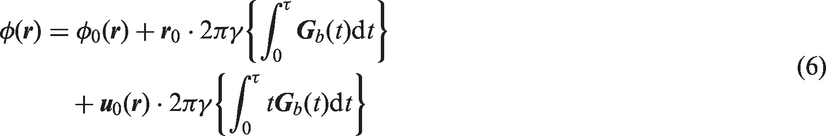
The experimental setup and key components are illustrated in Figure 1. The carpet and suction nozzle are placed in the reservoir, as shown in Figure 1(a). To prevent an undesired secondary flow around the nozzle, a perforated flow conditioner was utilized for the incoming flow to the reservoir. Double-sided tape was used to attach the carpet to the reservoir floor, and the nozzle was held by the mount attached to the reservoir wall.

Figure 1.

Experimental components and arrangements: (a) schematic of the reservoir with the carpet and the nozzle; (b) cross-sectional illustration of the carpet; (c) nozzle geometry and dimensions; (d) schematic of a closed-loop flow circuit installed for magnetic resonance velocimetry. MRI: magnetic resonance imaging.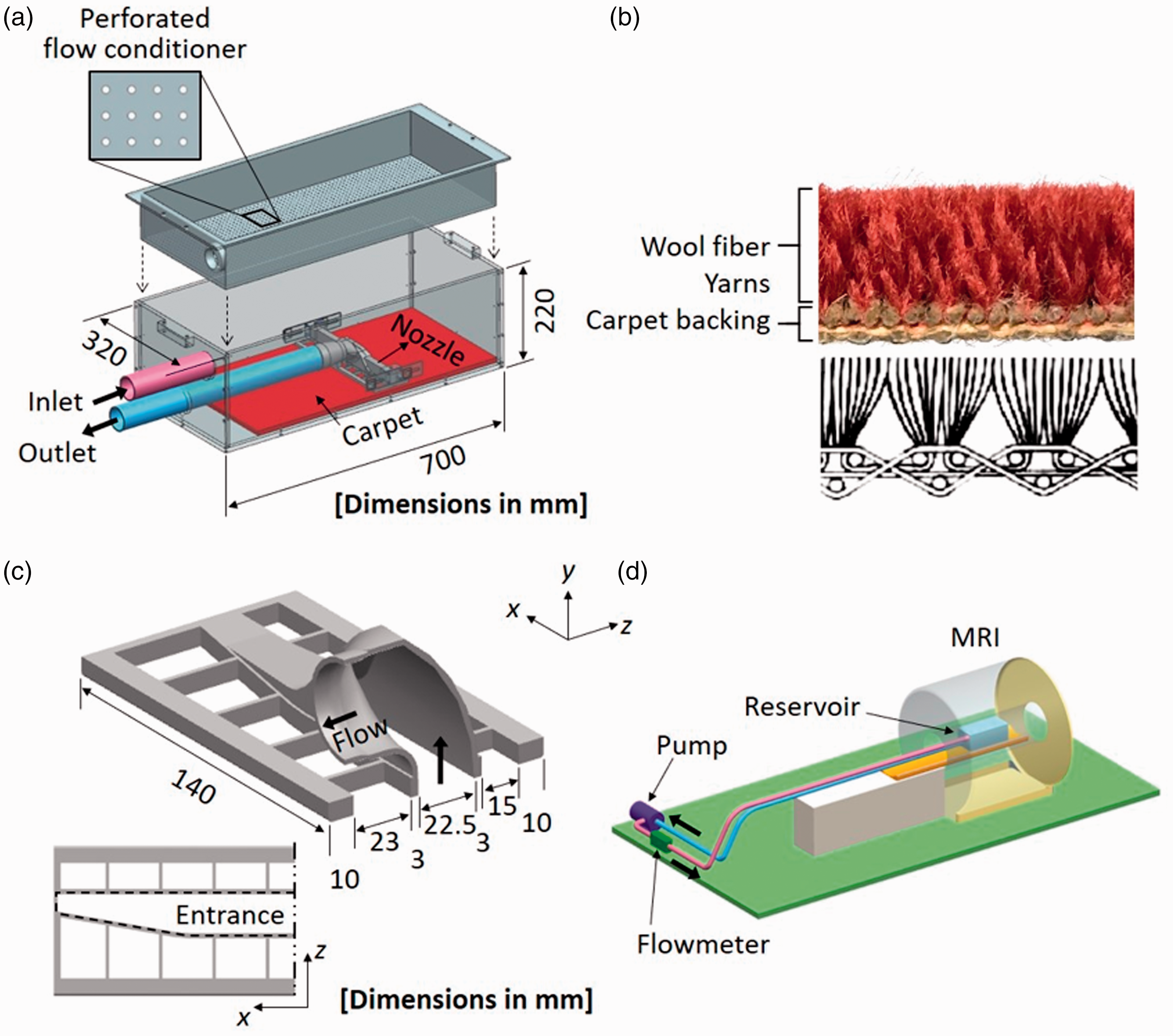

A Wilton carpet was used, which is a cut-pile carpet consisting of wool fiber yarns stitched on the surface of supporting material, as shown in Figure 1(b). The average height of the piles was 6.5 mm from the backing surface, and the average diameter of wool fibers was measured to be 40 µm. The bulk porosity of the pile region was estimated to be 0.86 by using two methods for cross-validation. One uses a formula that calculates the porosity by using the values in the carpet construction specification chart,⁴⁰ and the other uses a water-displacement volume measurement to experimentally estimate the porosity. According to the formula,⁴⁰ the bulk porosity for the pile region above the backing is calculated as

ɛ = 1 - 2 \cdot SD \cdot A_{y}

(10)

where ɛ is the porosity,

SD

is the stitch density (9.6 stitch/cm²), and

A_{y}

is the cross-sectional area of the yarn derived by dividing the weight of the yarn per length (0.001373 g/cm) by the fiber density (0.1909 g/cm³). The factor of two is multiplied because two fiber bundles protrude from a backing surface for a single stitch. The part of the formula

2 \cdot SD \cdot A_{y}

indicates the occupied portion of fibers for a unit area parallel to the backing surface. In addition to the calculation, the porosity was also experimentally investigated by measuring three types of volume: the volume of a bulk carpet sample (

V_{Bulk}

) which includes both solid (fibers and the carpet backing) and pores, the volume of solid (fibers and the carpet backing) in the sample (

V_{Solid}

), and the volume of the carpet backing (

V_{Backing}

). Then, the porosity can be calculated as

ɛ = \frac{V_{Bulk} - V_{Solid}}{V_{Bulk} - V_{Backing}}

(11)

where the numerator indicates the volume of only the pores in the sample, while the denominator represents the volume of both the pile and pores. A detailed description of the measurement process is as follows: firstly, a square piece of a carpet (20 mm × 20 mm) was cut by a sharp blade and its height was measured with a caliper (8.5 mm). The bulk volume was computed by assuming the sample as a cuboid. The measurement uncertainty is assumed to be 0.5 mm, considering that the bottom and top carpet surfaces are not perfectly flat. Next, the sample volume without pores was measured by using heat-curable polydimethylsiloxane (PDMS) liquid. PDMS was poured into a paper cup containing the sample and, then, the cup was placed inside a vacuum chamber to remove air bubbles and fill the pores with PDMS. Another sample was prepared using an identical weight of PDMS but without the carpet piece. Then, they were cured in an 80˚C oven for 2 hours and, then, the cups were peeled off. Since the volume difference of the two cured PDMS samples is equal to the volume of the carpet sample without pores, it was obtained by measuring the difference in the amount of water poured into a graduate cylinder with each sample to reach the same water level. The difference was measured as 900 ± 50 μl, where the water was poured with a 10 μl increment by using a precision pipette, and the level of the water was carefully inspected with human eyes. Finally, the volume occupied by the carpet backing was measured by removing all of the fibers from another carpet sample of equal size and using the water-level-matching approach. As a result, the volume was estimated to be 500 ± 50 μl. By inserting the volume measurements into Equation (11) and error propagation analysis, the porosity was estimated to be 0.86 ± 0.04, which showed a good agreement with the calculation with the carpet construction parameters (Equation (10)).

Figure 1(c) shows the geometry of the nozzle cut along its symmetric centerline. A vacuum cleaner manufacturer provided the geometry. A closed-loop flow circuit was installed for MR measurements, as shown in Figure 1(d). The circuit consisted of a water pump (PA–1000SS–T, Hanil Electrics, South Korea), which was controlled by an inverter system (SV015iG5A–1, LSIS, South Korea), and a turbine flowmeter (HF200, Nuritech, South Korea) to monitor the flow rate. All the experimental components except the pump were made of plastic materials to prevent magnetic field distortions. The pump was placed at a safe distance from the MRI scanner. A 40 mM copper sulfate aqueous solution was used as a working fluid to increase the signal-to-noise ratio (SNR).⁴¹ In order to suppress bubble formation in the flow circuit, the solution was degassed in a vacuum chamber at a pressure of 4 kPa for 10 minutes before it was poured into the reservoir.

MRV parameters and post-processing

We used a 3 Tesla human MRI scanner (Achieva 3 T, Philips, Netherlands). The accuracy of PC-MRI measurements has been validated for the same scanner for both laminar and turbulent flows in a circular pipe at various Reynolds numbers (Re).⁴¹ A 16-channel RF coil commonly used for imaging the human torso (XL-Torso coil, Philips, Netherlands) was wrapped around the reservoir to acquire MR signals from the flow. The voxel size was set to 1 × 0.5 × 1 mm³ in the x-, y-, and z-directions, resolving 13 velocity vectors across the carpet thickness. The field-of-view (FOV) was set to 336 × 14 × 128 mm³, which enclosed the entire carpet thickness and a finite volume above the carpet. A VENC of 100 cm/s was chosen for all encoding directions to avoid aliasing errors. The flip angle was set to 50° to achieve a SNR as high as possible. It was determined after measuring the static fluid in a bottle with similar MRV parameters but various flip angles (20°, 25°, 50°, and 70°). The echo time (TE) and repetition time (TR) were set to 6.4 and 15.4 ms, respectively, which were the shortest possible. The time required for measuring all three velocity components was approximately 15 minutes. The list of key parameters is outlined in Table 1.

Table 1.

Parameters for phase-contrast magnetic resonance imaging measurements

Parameter	Values
Scan mode	3D
Slice orientation	Coronal
FOV (x, y, z) [mm]	[336, 14, 128]
Voxel size (x, y, z) [mm]	[1, 0.5, 1]
Phase-encoding direction	Right to left
Flip angle	50°
Number of signal average	1
Flow compensation	Yes
VENC [cm/s]	x 100 cm/s
	y 100 cm/s
	z 100 cm/s

3D: three-dimensional; FOV: field-of-view.

In order to minimize an erroneous phase shift caused by the inhomogeneity of the magnetic field and induced eddy currents, PC-MRI measurements of identical sequence parameters were repeatedly carried out with the pump turned on and off. One dataset consisted of two flow-off and one flow-on data, which were measured in between the two flow-off datasets. The average of the two flow-off data was subtracted from the flow-on data. Four datasets of “flow on-and-off” were acquired and the averages of the four datasets are presented. The results were analyzed using in-house code written in MATLAB (Mathworks, Natick, MA, USA), and are depicted with the use of flow visualization software (Ensight, CEI, USA).

Results and discussion

MR signal magnitude

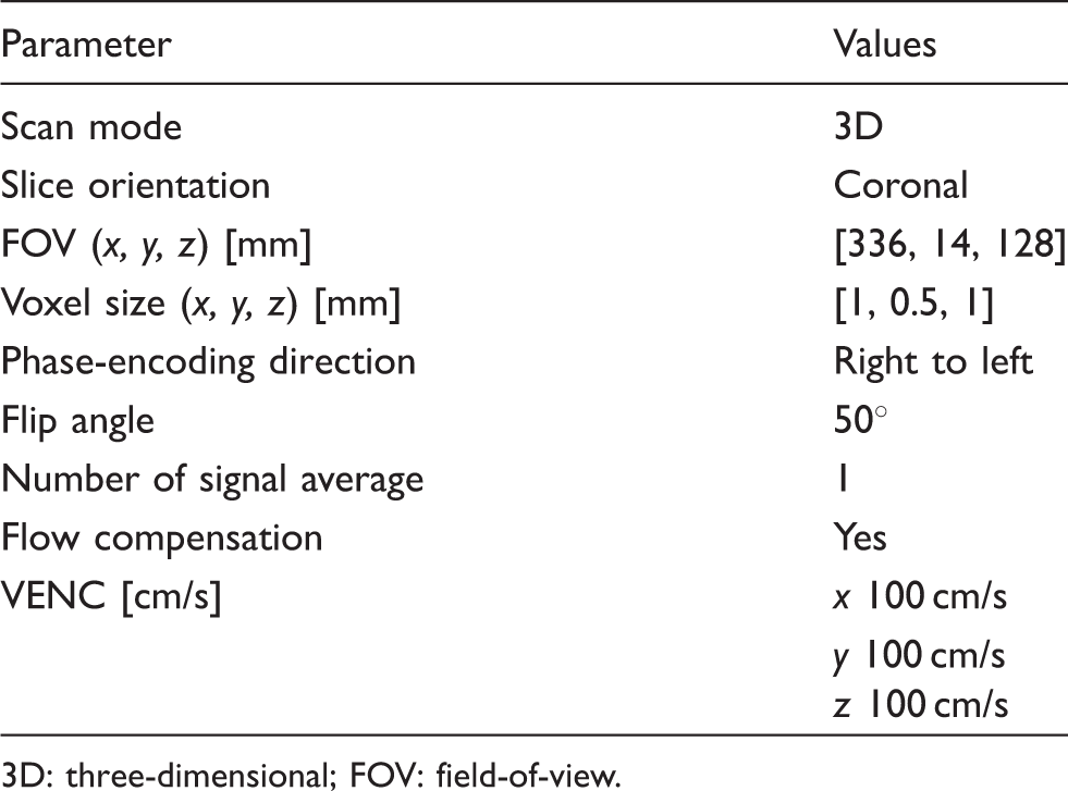
The spatial distribution of the signal magnitude in the MRV data provides the geometric information of an object in its FOV. The information is essential to reconstruct the flow geometry and assign the location of velocity vectors relative to the flow geometry. Figure 2(a) shows magnitude images at three selected FOV cross-sections. The dark area corresponds to the nozzle structure and the bright areas indicate the regions above the carpet that were occupied with fluid only. The region associated with the carpet produced a moderate magnitude because it was filled with both fluid and fibers. The reduction in the signal magnitude in the carpet was found to be approximately 40% of that in the region above the carpet. Ideally, this reduction ratio should be equal to the carpet porosity (0.86), because the signal magnitude in a voxel is linearly proportional to the volume of fluid and the porosity represents the fraction of fluid volume in a voxel as water filled the void spaces in the carpet. However, the reduction was greater than expected. This indicates that the decay rate of the MR signal for the voxels spatially colocalized with the carpet location was somehow larger than that for the voxels localized above the carpet. This extra signal loss may be induced by the co-presence of the carpet fibers (wool) and water. One possible explanation is that the magnetic susceptibility of the two materials could be different and it induces a microscopically inhomogeneous magnetic field near the carpet fibers, resulting in an extra signal loss due to the shortening of transverse relaxation time (T₂ relaxation).⁴²

Figure 2.

Spatial distribution of signal magnitude. (a) Cross-sectional images of the carpet. (b) Power spectrums of the spatial distribution of signal magnitudes along the z-axis averaged along the x-axis at various depths inside the carpet.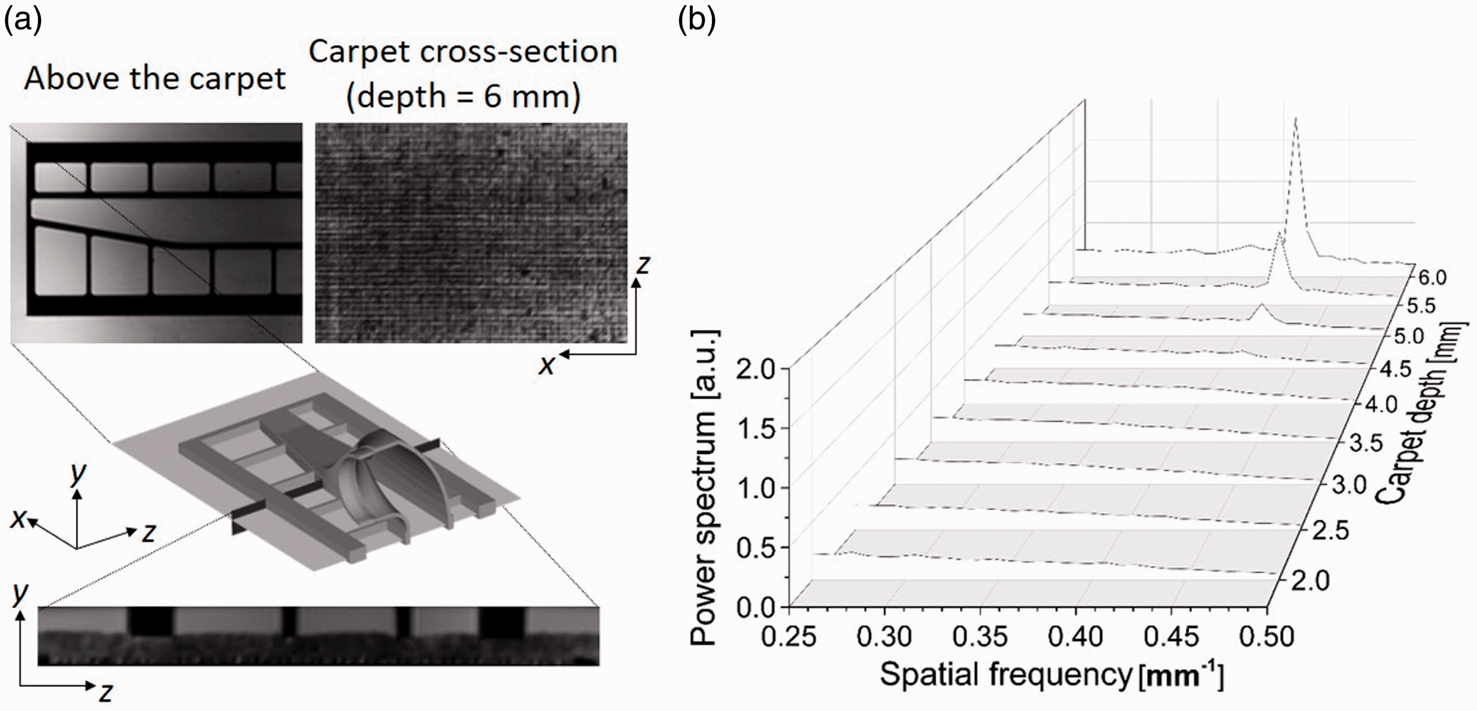

A checkered pattern was observed for the carpet close to the backing, as shown in the top-right image of Figure 2(a). This is because the yarns were repeatedly knitted using a square pattern. The characteristic length of the pattern was evaluated by the power spectrum of the magnitude image, as shown in Figure 2(b). The highest peak was measured at a wave number of 0.415 mm^–1 at a depth of 6 mm. This matches the knitting distance of the yarn in the range of 2.2–2.6 mm, measured at several locations with a caliper. The variation in the caliper measurements is probably due to the construction tolerance and the softness of the carpet backing structure. This power spectrum result indicates that large pores created by the knitting exist between the roots of the yarns. However, the large pores quickly disappeared as the depth decreased, noted by the disappearance of the peak. This confirms that the fibers were uniformly distributed and indicating that only small pores occupy the region above the depth of 4.5 mm.

Velocity field visualization

Before analyzing the velocity distribution in the carpet induced by the suction of the vacuum nozzle, raw velocity data obtained from MRV measurements were filtered and smoothed. Specifically, erroneous velocity vectors in the solid region were filtered by setting a threshold for the MR signal magnitude and by nulling the velocity below the threshold. In addition, the divergence-free smoothing (DFS) algorithm⁴³ was then applied to the remaining vectors to eliminate spurious velocity artifacts caused by the low SNR.

The overall accuracy of the velocity measurements was evaluated based on mass conservation analyses. A rectangular region-of-interest (ROI) was chosen to include the carpet below the nozzle, as shown in Figure 3. The ROI was placed to enclose the nozzle so that the flow rate coming into the ROI calculated by using MRV data should be equal to the suction flow rate measured by the flow meter. To evaluate MRV data at different locations in the carpet, the width and the height of the ROI were varied from 25 to 53 mm (2 mm increments) and from 5.5 to 7.5 mm (0.5 mm increments), respectively. The center of the ROIs was always aligned with the nozzle center and the top surface of ROIs was maintained at 1.5 mm above the carpet. As a result, the errors of the flow rate calculated with the MRV data against the flowmeter measurements were obtained from 50 ROIs, and Figure 3 shows the histogram of the errors. The results show that the errors are small. For example, the maximum error is only 3.5% and the average is 0.1% with 0.5% as the 95% confidence interval. In addition, when the error was computed before DFS application it was 1.8 ± 0.5% with the maximum of 4.5%. This indicates that DFS has altered the raw MRV data only by a little.

Figure 3.

Validation of magnetic resonance velocimetry (MRV) data. The count indicates the number of region-of-interests (ROIs) corresponding to a flow rate error. The error was defined as the relative error of the flow rate into a ROI (Q_in) calculated with the MRV data against the outflow rate (Q_out) measured with the flowmeter.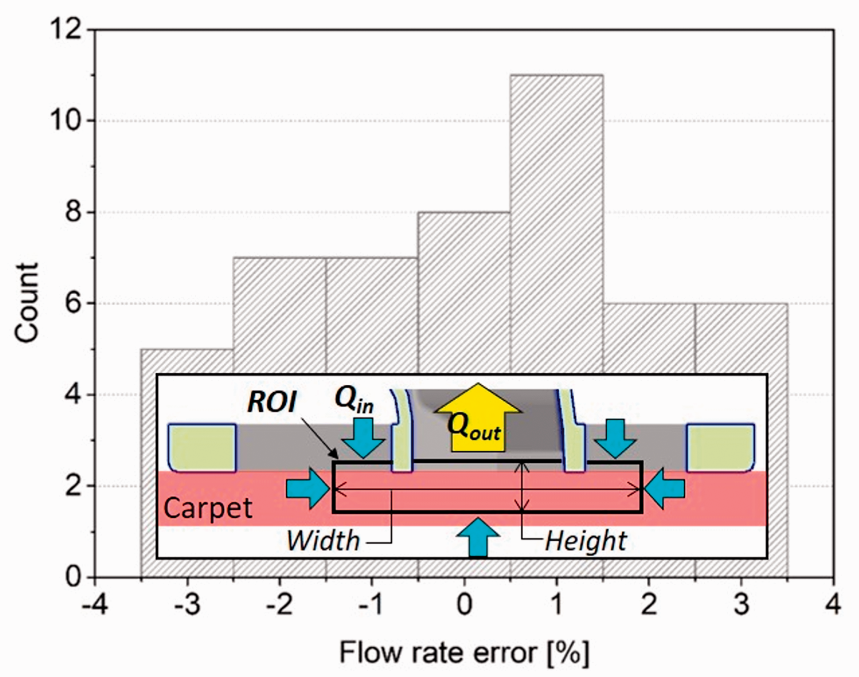

Figure 4 displays the velocity distribution induced by the vacuum cleaner nozzle. The 3C velocity vectors and magnitude contours are plotted in Figures 4(a) and (b). The contours indicate the magnitude of the velocity normalized by the average velocity at the nozzle exit (91.8 cm/s). The distribution of the velocity vectors clearly shows that the MRV is capable of visualizing flow in a porous medium like a carpet. The flow was found to be near and under the nozzle walls. In addition, a noticeable flow was induced in the carpet by the nozzle as far as 15 mm away from the nozzle wall, beyond which the flow within the carpet was weak (U / U_exit < 0.01).

Figure 4.

Velocity fields in the carpet measured by magnetic resonance velocimetry. (a) Corresponding three-component velocity vectors plotted on the selected planes. Note that the x–z plane corresponds to the velocity at the carpet depth of 1.5 mm. Arrows indicate the vector direction and the contours indicate the vector magnitude. (b) Surfaces of equal velocity magnitude. (c) Streamlines around the nozzle walls. 3D: three-dimensional.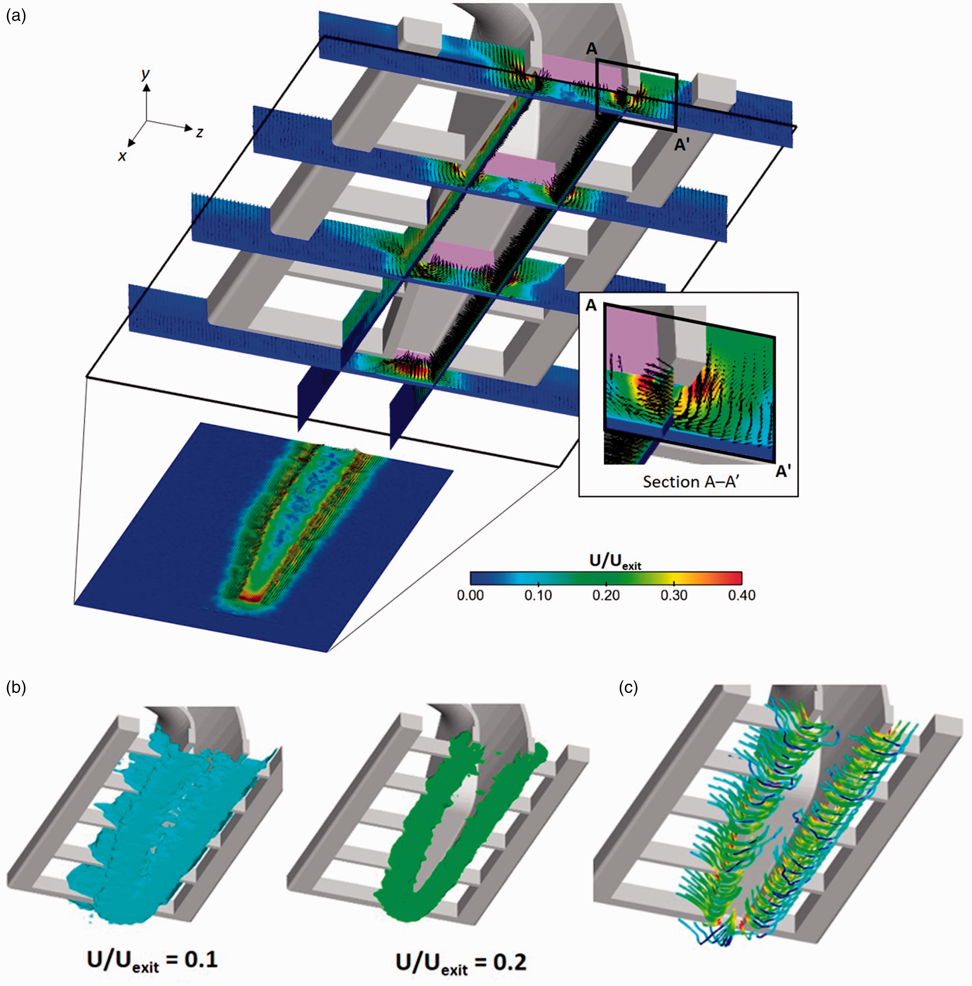

Interestingly, a region with decreased carpet velocities was observed under the center of the suction zone, as shown by the velocity contours in Figures 4(a) and (b). Such a low-velocity zone is more clearly observable by the velocity isosurfaces in Figure 4(c). While an isosurface of a relatively high velocity (U / U_exit = 0.2) is located underneath the nozzle walls, only an isosurface of a low-velocity (U / U_exit = 0.1) is found to exist in between the high-velocity isosurfaces. Along the transverse centerline, the velocity appeared to be lower than that at the isosurface. This was caused by the fact that most of the flow was inhaled close to the nozzle inner wall, as depicted by the streamline plot in Figure 4(c). The origins of the streamlines (or pathlines) were chosen above the carpet outside of the nozzle to illustrate the trajectory of the surrounding fluid that flowed into the nozzle. According to the streamlines, the flow formed sharp U-turns under the nozzle wall instead of penetrating into the central area by inertia. This was due to the anisotropic structure of the carpet fiber alignment. The fiber alignment imposed a large resistance to the fluid flow in the direction perpendicular to the fibers, while a relatively small resistance was imposed to the parallel flow. As a result, the low-velocity region appeared near the center under the nozzle.

For the purpose of cleaning, it is desirable to induce a flow in the carpet that is as deep as possible to remove dust particles that exist near the surface of the carpet backing. The investigation of the velocity profiles in the direction of the depth of the carpet would provide useful insight on the removal force experienced by dust particles. Figure 5 shows the velocity distribution averaged along the four faces of the nozzle wall in the carpet, namely, the front center, front side, rear center, and the rear side right underneath the wall. Overall, the velocity of the horizontal component increased to reach a maximum magnitude near the depth of 2–3 mm. It then decreased gradually at increased depths. The sharp U-turn of the flow around the nozzle wall caused such a velocity profile in the carpet as that noted in the close-up window in Figure 4(a). At a depth of 6 mm, the velocities in all the regions were reduced to half of their maximum velocity. This is probably be attributed to the abrupt U-turn of flows under the thin nozzle wall. In addition, a regional difference in flow strength was observed. It was found that a stronger flow was induced at the center rather than at the side, and at the front rather than at the rear. The difference between the center and side could be related to the nozzle outlet location, which is at the center. It induces low pressure at the center, causing a stronger suction than at the side. The difference between the front and the rear may be related to the direction of flow exiting the nozzle, which is toward the back, as shown in Figure 1(a). It can be inferred from the nozzle geometry (Figure 1(c)) that flows coming from the rear experience a curvature greater than those from the front, and the higher the curvature of streamlines the more difficult the fluid flow.

Figure 5.

Velocity profiles underneath the nozzle walls with respect to the depth of the carpet. Velocity profiles were averaged over an area below the four nozzle faces indicated by the arrows, which also indicate the directions of velocity considered.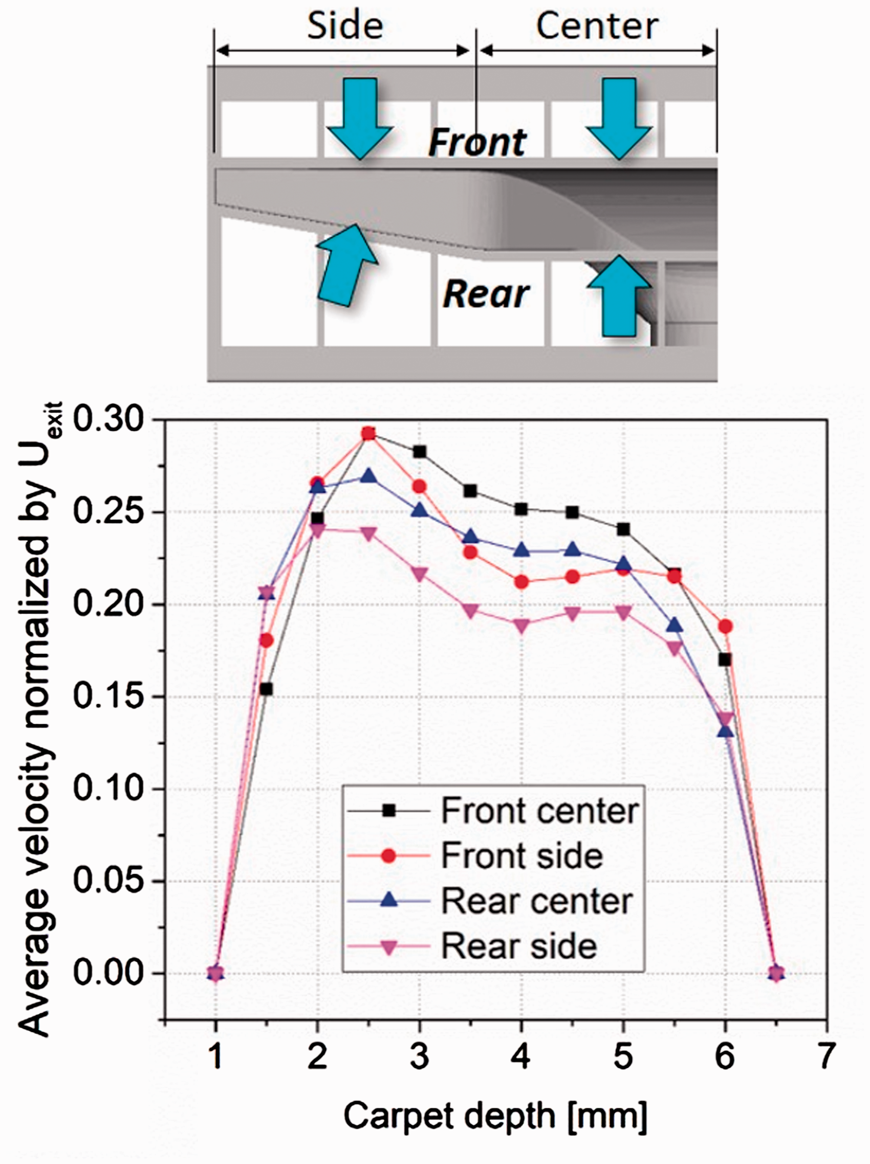

Pressure field estimation

The pressure distribution in a porous medium provides useful information because it is closely related to the drag exerted on an object within a flow field or the frictional loss in a medium. In particular, the drag is the driving force required to clean the dust particles in the carpet. With the 3D 3C velocity data obtained by MRV, the pressure distribution in the carpet could be estimated by a two-step process: (a) computation of the pressure gradient in the carpet and (b) integration of the gradient.

To determine the pressure gradient, three assumptions were postulated:

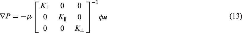
every voxel in the carpet was occupied by the same number of fibers;

pressure drops due to the inertia of the flow can be neglected;

the permeability of the carpet along the direction parallel to the fibers was twice as large as that along the normal direction to the fibers.⁴⁴

The first assumption would be invalid for (a) the voxels that are near the carpet backing because the pores are larger than the voxels, and (b) the voxels close to the carpet surface where a part of a voxel may occupy the region above the carpet. Therefore, the region of the carpet at depths ranging from 1.5 to 4.5 mm was chosen to be the estimation domain. The validity of the second assumption can be evaluated with an interstitial Re, which is defined as

Re = \frac{ρ U d_{f}}{μ}

(12)

where U is the velocity magnitude at the voxel, μ is the dynamic viscosity of the fluid, ρ is the density of water, and

d_{f}

is the average fiber diameter, which represents a characteristic length of a fibrous porous media.^45,46 It was found that 95% of the voxels had Re < 10 in this domain. This implies that the contribution of an inertial drag to the pressure loss would be minor, as compared to the viscous drag.⁴⁷ Therefore, the pressure gradient was calculated based on Darcy's law

\nabla P = - μ \begin{matrix} [\begin{matrix} K_{⊥} & 0 & 0 \\ 0 & K_{∥} & 0 \\ 0 & 0 & K_{⊥} \end{matrix}]^{- 1} φ u \end{matrix}

(13)

where P is the static pressure,

u

is the velocity measured by MRV, and φ is the porosity of the carpet. Note that

K_{⊥}

and

K_{∥}

indicate the permeabilities in the directions normal and parallel to the fiber, respectively. Equation (13) is further simplified by defining a dimensionless pressure such that

\tilde{P} = \frac{K_{⊥}}{μ φ U_{exit}} P

(14)

Accordingly

\nabla \tilde{P} = - \begin{matrix} [\begin{matrix} 1 & 0 & 0 \\ 0 & α & 0 \\ 0 & 0 & 1 \end{matrix}] \frac{u}{U_{exit}} \end{matrix}

(15)

where α is the permeability ratio, defined as

K_{⊥} K_{∥}

. The final assumption plays a role in setting the value of α to 0.5 based on the theoretical derivation of permeability for the randomly distributed parallel cylindrical array.⁴⁴

In the second step used to determine the pressure distribution, the pressure gradients were integrated by the ODI method.⁴⁸ This method was reported to estimate a two-dimensional (2D) pressure field using 2D velocity field data. It integrated the given pressure gradients along numerous lines at various directions using the initial pressure values, and iteratively repeated the integration until the entire pressure field converged.

We have expanded the ODI method for applicability to a 3D field. To create 3D integration paths, lines were randomly created by connecting two of the virtual points uniformly distributed on a sphere, tightly enclosing a given 3D hexahedral velocity domain. The voxels along the integration line were selected to calculate a pressure gradient along the line, as shown in Figure 6(a). After integrating the pressure gradients along all the lines, multiple pressure values were accumulated and averaged at every voxel. This process was repeated until the pressure converged over the entire domain between consecutive iterations. For validation, we compared the pressure obtained by the 3D ODI method against the data elicited from direct numerical simulations (DNSs) for an isotropic turbulent flow.^49,50 Note that we introduced 10% Gaussian random errors to the DNS data before applying the ODI method to simulate experimental noise in MRV. Figure 6(b) shows the pressure fields reconstructed by the 3D ODI method and the DNS. Relative errors are also shown in this figure on the plane with the maximum error. The results showed that the 3D ODI method accurately reconstructed the pressure with the average and maximum errors of 0.8% and 2.5%, respectively. The error was defined as the difference in the pressure between the DNS and ODI results divided by the difference of the maximum and minimum pressures in the DNS data.

Figure 6.

Schematic of a three-dimensional (3D) omni-directional integral (ODI) integration path and validation results: (a) illustration of an integration path and voxels on the integration path in the 3D data domain; (b) direct numerical simulation (DNS) and 3D ODI reconstructed pressure contours.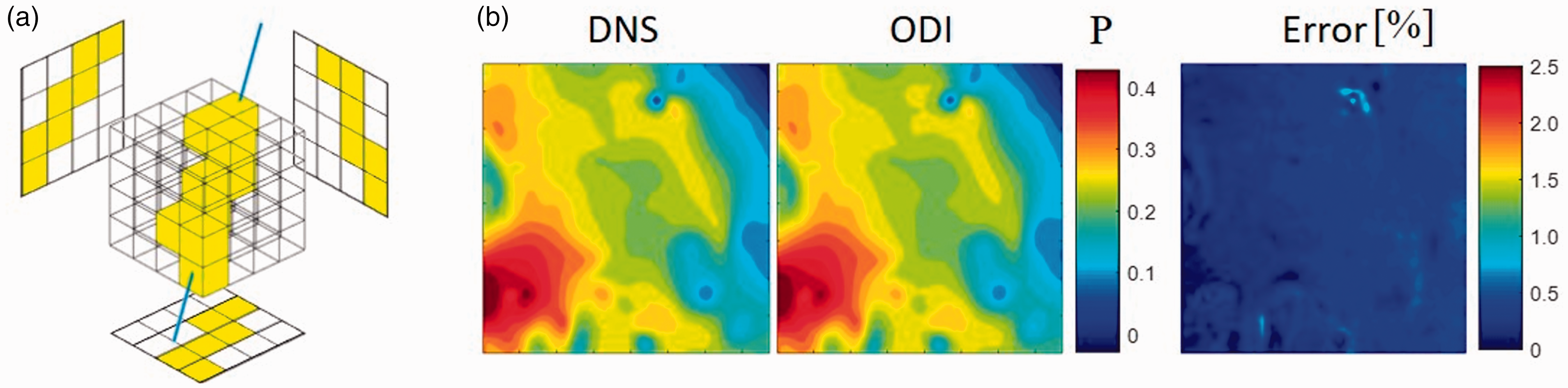

Figure 7 shows the pressure field in the carpet estimated by the 3D ODI method. The estimation domain consisted of 148 × 9 × 79 voxels along the x-, y-, and z-axes. The number of integration paths was 1,936,430 and the total computational time was approximately 17 minutes per iteration using MATLAB parallel processing with 20 CPU cores (Xeon E5–2680V2, 2.80 GHz, a clock speed of 22.4 Gflops, Intel, USA). The pressure converged to a degree of 10⁻³ after 60 iterations. Note that the ODI method estimated the pressure relative to a reference location. We set the farthest corner point from the nozzle as the reference at which the pressure could be equal to the ambient zero pressure. The pressure contour revealed that the pressure drop was most significant under the edges of the nozzle walls, thereby converting pressure to kinetic energy. As discussed previously for the velocity distribution, the pressure distribution also confirmed that the center region under the nozzle footprint had low and uniform pressure. It should be noted that a low-pressure region would be undesirable in a carpet from a nozzle design point-of-view because dust particles would experience a minimal force in such a region.

Figure 7.

Dimensionless pressure distribution within the carpet: (a) contours of pressure on the selected planes; (b) surfaces of the identical pressure values. The pressure was estimated relative to the reference point located at the corner of the domain.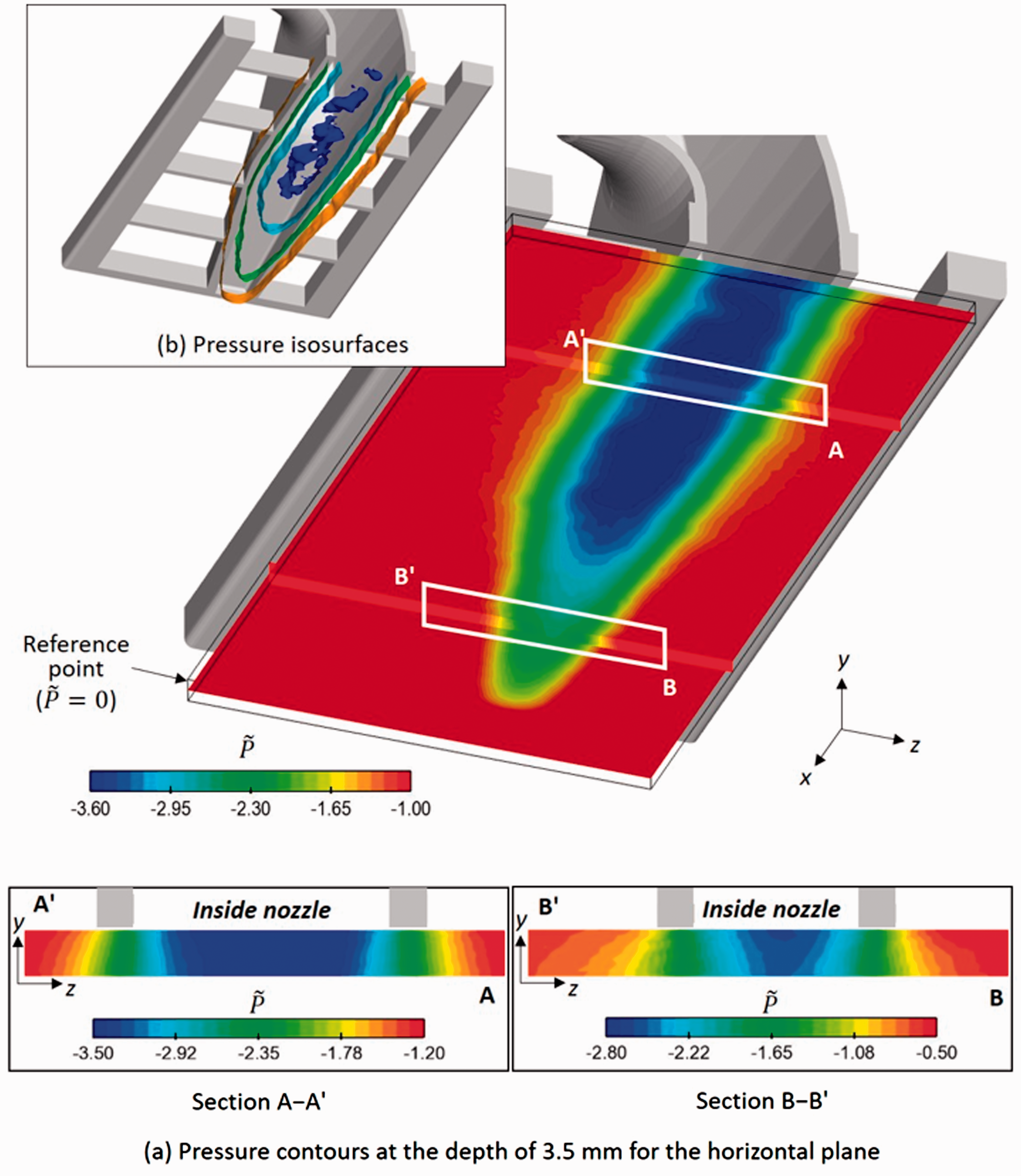

Conclusions

This study addressed the utilization of MRV to quantitatively visualize 3C velocity vectors of a flow in a 3D porous medium, and the use of a 3D ODI method to estimate the pressure field. The flow in a carpet induced by the suction of a vacuum cleaner nozzle was accurately measured by PC-MRI, and the 3D ODI method in combination with MRV revealed the 3D distribution of pressure. Accordingly, we identified a flow-dominant region in the carpet and characterized the flow in the carpet. The velocity vector plots and the streamlines clearly depicted the flow paths in the carpet. It was found that the flow pattern formed a U-turn under the nozzle walls owing to the anisotropic alignment of the carpet fibers and generated a region of low-velocity and low-pressure under the center of the nozzle footprint. We believe that the combination of MRV and the 3D ODI method would uncover complex characteristics of flow in textile materials.

Footnotes

Declaration of conflicting interests

The authors declare that there are no potential conflicts of interest with respect to the research, authorship, and/or publication of this article.

Funding

The authors disclosed receipt of the following financial support for the research, authorship, and/or publication of this article: This work was supported by the National Research Foundation of Korea (NRF) grant funded by the Korean government (No. 2016R1A2B3009541) and a research fund from Hanyang University (HY–2018).

References

Turan

Okur

. Prediction of the in-plane and through-plane fluid flow behavior of woven fabrics. Text Res J 2013; 83: 700–717.

Tamayol

Wong

Bahrami

. Effects of microstructure on flow properties of fibrous porous media at moderate Reynolds number. Phys Rev E 2012; 85: 026318.

Pradhan

Das

Chattopadhyay

, et al. Effect of 3D fiber orientation distribution on transverse air permeability of fibrous porous media. Powder Technol 2012; 221: 101–104.

Yarlagadda

Yoganathan

. Experimental studies of model porous media fluid dynamics. Exp Fluids 1989; 8: 59–71.

Huang

Capart

, et al. Optical measurements of pore geometry and fluid velocity in a bed of irregularly packed spheres. Exp Fluids 2008; 45: 309–321.

Lachhab

Zhang

Muste

. Particle tracking experiments in match-index-refraction porous media. Groundwater 2008; 46: 865–872.

Moroni

Cushman

. Statistical mechanics with three-dimensional particle tracking velocimetry experiments in the study of anomalous dispersion. II. Experiments. Phys Fluids 2001; 13: 81–91.

Peurrung

Rashidi

Kulp

. Measurement of porous medium velocity fields and their volumetric averaging characteristics using particle tracking velocimetry. Chem Eng Sci 1995; 50: 2243–2253.

Sen

Nobes

Mitra

. Optical measurement of pore scale velocity field inside microporous media. Microfluid Nanofluid 2012; 12: 189–200.

10.

Agelinchaab

Tachie

Ruth

. Velocity measurement of flow through a model three-dimensional porous medium. Phys Fluids 2006; 18: 017105.

11.

Khayamyan

Lundström

Gren

, et al. Transitional and turbulent flow in a bed of spheres as measured with stereoscopic particle image velocimetry. Transp Porous Media 2017; 117: 45–67.

12.

Patil

Liburdy

. Flow structures and their contribution to turbulent dispersion in a randomly packed porous bed based on particle image velocimetry measurements. Phys Fluids 2013; 25: 113303.

13.

Patil

Liburdy

. Flow characterization using PIV measurements in a low aspect ratio randomly packed porous bed. Exp Fluids 2013; 54: 1497.

14.

Roman

Soulaine

AlSaud

, et al. Particle velocimetry analysis of immiscible two-phase flow in micromodels. Adv Water Resour 2016; 95: 199–211.

15.

Wang

. An experimental investigation of the permeability in porous chip formed by micropost arrays based on microparticle image velocimetry and micromanometer measurements. J Fluids Eng 2017; 139: 021108.

16.

Zhong

Currie

James

. Creeping flow through a model fibrous porous medium. Exp Fluids 2006; 40: 119–126.

17.

Khayamyan

Lundström

Hellström

JGI

, et al. Measurements of transitional and turbulent flow in a randomly packed bed of spheres with particle image velocimetry. Transp Porous Media 2017; 116: 413–431.

18.

Blois

Barros

Christensen

. A microscopic particle image velocimetry method for studying the dynamics of immiscible liquid–liquid interactions in a porous micromodel. Microfluid Nanofluid 2015; 18: 1391–1406.

19.

Imhoff

Jaffe

Pinder

. An experimental study of complete dissolution of a nonaqueous phase liquid in saturated porous media. Water Resour Res 1994; 30: 307–320.

20.

Khalili

Basu

Pietrzyk

. Flow visualization in porous media via positron emission tomography. Phys Fluids 1998; 10: 1031–1033.

21.

Chang

Watson

. NMR imaging of flow velocity in porous media. AIChE J 1999; 45: 437–444.

22.

Boyce

Rice

Sederman

, et al. 11-interval PFG pulse sequence for improved measurement of fast velocities of fluids with high diffusivity in systems with short T2∗. J Magn Reson 2016; 265: 67–76.

23.

Chen

Marble

, et al. Flow imaging of fluids in porous media by magnetization prepared centric-scan SPRITE. J Magn Reson 2009; 197: 1–8.

24.

Romanenko

Xiao

Balcom

. Velocity field measurements in sedimentary rock cores by magnetization prepared 3D SPRITE. J Magn Reson 2012; 223: 120–128.

25.

Watson

. Determining spatial distributions of permeability. Transp Porous Media 2011; 86: 385–414.

26.

Onstad

Elkins

Medina

, et al. Full-field measurements of flow through a scaled metal foam replica. Exp Fluids 2011; 50: 1571–1585.

27.

Huang

Mikolajczyk

Küstermann

, et al. Adapted MR velocimetry of slow liquid flow in porous media. J Magn Reson 2017; 276: 103–112.

28.

Ren

Stapf

Blümich

. Magnetic resonance visualisation of flow and pore structure in packed beds with low aspect ratio. Chem Eng Technol 2005; 28: 219–225.

29.

Yang

Scheibe

Richmond

, et al. Direct numerical simulation of pore-scale flow in a bead pack: comparison with magnetic resonance imaging observations. Adv Water Resour 2013; 54: 228–241.

30.

Carr

Beckham

Spiess

, et al. Nuclear-magnetic-resonance imaging of water distributions in loop-pile nylon carpet tiles. J Text Inst 1998; 89: 436–440.

31.

Lee

Carr

Beckham

, et al. A model of through-air drying of tufted textile materials. Int J Heat Mass Transfer 2002; 45: 357–366.

32.

Lee

Carr

Leisen

, et al. Through-air drying of unbacked tufted carpets. Text Res J 2001; 71: 613–620.

33.

Leisen

Beckham

. Quantitative magnetic resonance imaging of fluid distribution and movement in textiles. Text Res J 2001; 71: 1033–1045.

34.

Leisen

Hojjatie

Coffin

, et al. In-plane moisture transport in paper detected by magnetic resonance imaging. Drying Technol 2001; 19: 199–206.

35.

Markl

Frydrychowicz

Kozerke

, et al. 4D flow MRI. J Magn Reson Imaging 2012; 36: 1015–1036.

36.

Elkins

Alley

. Magnetic resonance velocimetry: applications of magnetic resonance imaging in the measurement of fluid motion. Exp Fluids 2007; 43: 823–858.

37.

Haacke

Brown

Thompson

, et al. Magnetic resonance imaging: physical principles and sequence design, New York: Wiley-Liss, 1999.

38.

Liang Z-P and Lauterbur PC. Principles of magnetic resonance imaging: a signal processing perspective. Piscataway: SPIE Optical Engineering Press, 2000.

39.

Pelc

Bernstein

Shimakawa

, et al. Encoding strategies for three-direction phase-contrast MR imaging of flow. J Magn Reson Imaging 1991; 1: 405–413.

40.

Zhou

Warner

. Pore sizes in carpet. Text Res J 1999; 69: 423–430.

41.

Lee

Cho

J-H

, et al. Validation of magnetic resonance velocimetry for mean velocity measurements of turbulent flows in a circular pipe. J Mech Sci Technol 2017; 31: 1275–1282.

42.

Schenck

. The role of magnetic susceptibility in magnetic resonance imaging: MRI magnetic compatibility of the first and second kinds. Med Phys 1996; 23: 815–850.

43.

Wang

Gao

Wang

, et al. Divergence-free smoothing for volumetric PIV data. Exp Fluids 2016; 57: 15.

44.

Shou

Fan

Ding

. Hydraulic permeability of fibrous porous media. Int J Heat Mass Transfer 2011; 54: 4009–4018.

45.

Jackson

James

. The permeability of fibrous porous media. Can J Chem Eng 1986; 64: 364–374.

46.

Tamayol

Khosla

Gray

, et al. Creeping flow through ordered arrays of micro-cylinders embedded in a rectangular minichannel. Int J Heat Mass Transfer 2012; 55: 3900–3908.

47.

Huang

Ayoub

. Applicability of the Forchheimer equation for non-Darcy flow in porous media. SPE J 2008; 13: 112–122.

48.

Liu

Katz

. Vortex-corner interactions in a cavity shear layer elucidated by time-resolved measurements of the pressure field. J Fluid Mech 2013; 728: 417–457.

49.

Perlman

Wan

, et al. A public turbulence database cluster and applications to study Lagrangian evolution of velocity increments in turbulence. J Turbul 2008; N3: 11–29.

50.

Perlman E, Burns R, Li Y, et al. Data exploration of turbulence simulations using a database cluster. In: Becky V (ed.) proceedings of the 2007 ACM/IEEE conference on supercomputing, Reno, Nevada, USA, 10–16 November, 2007, paper no. 23. New York, USA: ACM.