Drink what you can pay for: Financing infrastructure in a fragmented water system

Abstract

Chinese

The article investigates the relationship between environmental violations and water utility infrastructure investment in the Houston metropolitan area through a lens of institutional fragmentation. Special purpose water districts are highly capital-intensive service jurisdictions, which makes them extremely dependent on local fiscal capacity. Fiscal capacity is also important for a water district’s ability to respond to performance failures, particularly regulatory violations. Resource base, however, is unevenly distributed between special purpose water districts in the highly fragmented Houston metro area. Therefore, while capital investments may significantly covary with fiscal capacity, not all water districts are expected to be capable of making needed infrastructure investment when problems arise. There are two major policy-relevant findings that we offer in the article. Institutional fragmentation in relatively more affluent areas does not impede the ability to invest in capital infrastructure related to both service pressures and regulatory violations. However, such ability is limited in relatively less affluent areas, where the fiscal capacity to respond to service delivery problems is limited.

Keywords

capital investment drinking water fiscal capacity institutional fragmentation service delivery

Introduction

Metropolitan areas exhibit considerable variation in public services and policy outcomes at the neighbourhood level (Chen et al., 2011; Downey 2007). Much of this heterogeneity is attributable to horizontal and functional fragmentation in which local government responsibilities are divided amongst small and/or specialised authorities (Parks and Oakerson, 2000). One obvious, but often overlooked, implication of urban fragmentation is that the institutional capacity of each service provider is tied to the economic and fiscal capacity of the local service area – providers rely upon a combination of service revenues and taxes to fund operations and capital improvements. Thus, because wealth can differ on a neighbourhood-by-neighbourhood basis, local service providers likewise can differ greatly in terms of their responsiveness and ability to marshal the resources necessary to perform core functions (Mullin, 2009).

The article explores this phenomenon in the context of water infrastructure investment. While a body of literature has focused on how different drinking water providers perform with respect to regulatory violations and enforcement (Konisky and Teodoro, 2016; Rubin, 2013), it is less well understood how effectively providers serving economically disparate neighbourhoods can respond to service delivery challenges. Using the case of more than 500 special purpose water supply districts in the Houston, Texas metropolitan statistical area (MSA),¹ we investigate the relationship between United States Safe Drinking Water Act (SDWA) violations (used as an indicator of investment need) and subsequent capital infrastructure investments by these public water providers, conditional on resource capacity. Water districts are a useful case because they are a significant source of service delivery fragmentation in many metropolitan regions; these entities can be hyper-localised, serving specific local areas or neighbourhoods, and thus vary considerably in their economic and fiscal capacity (Mullin, 2009). Given the differences in each system’s resource base, we seek to understand the ability of service providers to make necessary capital investments in response to regulatory violations.

In what follows, we discuss the context of this study – drinking water provision and regulation – and describe the case at hand. We then discuss the existing theory and evidence concerning the special districts and highly fragmented institutional environments, and advance hypotheses regarding how fiscal and economic capacity impacts capital investment by service providers. We test these hypotheses by modelling infrastructure investment as a function of regulatory violations and institutional capacity over an eight-year period. Water service districts with high fiscal capacity are found to be more likely to make infrastructure investments after committing a major violation; this raises important concerns about how institutional fragmentation within metropolitan areas can decrease equity when public service delivery is constrained by local resource capacity.

Background and case selection

The SDWA is a useful device for examining how institutional capacity can constrain regulatory compliance efforts because it requires a relatively common set of behaviours from all providers regardless of location, type or size (Teodoro and Switzer, 2016).² Under the SDWA, utility systems are required to self-monitor and report. Utilities are required to conduct regular sampling and testing, to provide adequate and timely public notice of violations and to produce a yearly report that summarises system performance. Failures to conduct monitoring and testing, or to adhere to public notice and administrative reporting requirements, are classified by the EPA as monitoring and reporting, or public notice, violations. Following the convention of Teodoro and Switzer (2016), we label these as management violations since they reflect procedural compliance but do not necessarily reflect actual water conditions. In contrast, health violations occur when systems exceed maximum contaminant levels, exceed maximum levels of treatment chemicals or fail to adhere to established treatment techniques. Management violations relate to administrative functions rather than the condition and quality of capital infrastructure. Thus, management violations are not expected to precipitate capital investment. In contrast, health violations attributable to contaminants or treatment problems are addressed by the capital maintenance of existing systems or investing in water purpose infrastructure.³

As in the Houston case, most community water systems regulated under the SDWA⁴ are relatively small: more than 90% of regulated systems in the US have fewer than 10,000 customers (Levin et al., 2002). For smaller systems, the capital costs of investing in water supply infrastructure can be prohibitive or unattainable (Mullin, 2009). Thus, while existing evidence indicates that small service providers are not necessarily any more likely than large providers to commit major health violations (Rubin, 2013), capacity constraints do limit providers’ ability to access necessary resources and make major capital investments when necessary (Teernstra, 1993).

Water provision in the Houston metropolitan region is accomplished through a mix of direct service from municipalities, public corporations, special purpose water districts and private operators. System capacity is a focal issue because, for the most part, providers must rely on their own resources to finance service provision. State programs such as the Texas Drinking Water State Revolving Fund (DWSRF) Loan Program provide below market interest rate loans and loan forgiveness to support critical investments. Similarly, the Texas Economically Distressed Areas Program (EDAP) provides grants and loan-grant combinations to fund improvements in particularly needy jurisdictions. However, these programmes are small. For instance, only two water providers in the Houston MSA received EDAP funding in fiscal year 2016 (out of more than 1400 public and private regulated providers).⁵ Thus, tax revenues and service fees are the primary sources of funds.

Of the approximately 6.5 million people in the Houston area served by community water systems regulated under the SDWA, 40% receive their water from special purpose districts.⁶ The array of special water districts in the region presents a unique opportunity to closely examine the association between fiscal capacity, service performance and infrastructure investment by service providers. While information on municipal water systems is included in general purpose government financial reports, it is often challenging to parse out cleanly the cash flows used for water service provision. This is not the case for special districts, which are required to file yearly financial audits with TCEQ that detail their revenues, expenditures and fund balance.⁷ Moreover, unlike for private providers and public corporations, the Texas Bond Review Board (TBRB) maintains a database of debt issuance by special purpose districts.⁸ Thus, while we expect that fragmentation impacts the service capacity of all provider types, water districts are an opportune case because we can track both their yearly finances and debt issuance events. We focus exclusively on the more than 500 active municipal utility districts (MUDs), freshwater supply districts (FWSDs) and water control and improvement districts (WCIDs).⁹

Theoretical framework and hypotheses

As stated above, the fundamental premise of this article is that the ability of a given public service provider to carry out intended functions is dependent upon local ability to pay. For the most part, local providers in a given urban region face consistent operational requirements and procedural constraints. Providers are expected to meet common service expectations and bear similar water storage, transportation and treatment costs in spite of the fact that local service populations can differ greatly in their ability to pay for it. Thus, fragmentation can create ‘diseconomies of scale’ whereby small providers lack the fiscal capacity to maintain service quality (Hooghe and Marks, 2003; Jimenez and Hendrick, 2010).

Fiscal capacity is ‘the capacity of a … [provider] to fund its own water supply functions and offer production resources to its neighbors’ (Mullin, 2010: 152). Fiscal capacity is particularly central to water service provision because it requires highly capital-intensive infrastructure (Mullin, 2009). Size is not just an issue with respect to fixed capital: smaller jurisdictions even pay an interest rate penalty on their debt (Simonsen et al., 2001) and can lack technical expertise (Teodoro and Switzer, 2016). Furthermore, the issue of scale is compounded by the tendency for disadvantaged areas to have pressing service improvement needs (Teodoro and Switzer, 2016). Large-scale providers can cross-subsidise across local areas, in effect smoothing across rich and poor neighbourhoods. In contrast, the ability of small-scale providers to respond to service needs is more directly tied to the economic and fiscal capacity of the local neighbourhood (Jimenez, 2014; Meyer and Konisky, 2007).

The relationship between fragmentation, government size and service outcomes is, however, not always straightforward. Vertical fiscal imbalances, interjurisdictional competition and overlapping governments (Greer, 2014; Jimenez, 2015; Karuppusamy and Carr, 2012) make local fiscal outcomes (such as debt levels, interest payments or tax and expenditure structures) highly variable. Fiscal outcomes are thus contingent on institutional incentives and constraints that govern vertical and horizontal fiscal relationships between governments (Karuppusamy and Carr, 2012).

In considering how providers are able to access needed funds, we distinguish between economic and fiscal capacities as related, but distinct, factors. Economic capacity refers to the general economic base in a region. For example, one common measure of the economic base is property values. Economic capacity and the diversity of an economic base has been shown to influence both debt affordability and credit rating agency decisions (Hildreth and Miller, 2002). While economic capacities (often proxied by median home prices or percent living in poverty) are assumed to be important for service capacity, water providers are limited in their ability to leverage this base fully. Allocation agreements negotiated with general purpose governments limit the ability of districts to draw from their economic base (e.g. via taxes) and set forth rules for infrastructure financing. This revenue generation capability is referred to as fiscal capacity, represented by the tax and service revenues that districts generate.

Tax and service revenues are a more direct indicator of a district’s financial capabilities because they reflect both underlying economic capacity and the extent to which a given district can leverage this base to generate fiscal capacity. Fiscal capacity is also dependent on the excess fiscal slack available for non-recurring and unanticipated events such as the urgent need to address SDWA health violations. Existing literature on fiscal slack, measured by assessing fund balances, shows that organisations are better able to withstand major external shocks by relying on such extra fiscal cushions (Marlowe, 2005). Fiscal slack would also be indicative of superior fiscal capacity, which is perceived very positively in the debt market and allows premium access to capital financing (Johnson et al., 2014).¹⁰

As of the end of 2016, 475 of the 527 districts in our sample qualify as small systems under the SDWA. While small systems can apply for waivers if they are unable to comply with particular rules, they are not exempted from addressing major health issues such as bacterial contamination or significant treatment problems (EPA Office of Water, 2004). The implication of such a highly fragmented, localised service delivery regime is that districts vary considerably in both their economic and fiscal capacity and thus not all districts have the same ability to access capital financing.

Hypothesis 1: Water districts with greater fiscal capacity are more likely to make debt-financed capital investment.

Furthermore, health violations under the SDWA relate to problems with water contamination or treatment failures; these types of problems can be evidence of aging systems, failing technology, insufficient infrastructure or maintenance shortfalls. These types of problems are unlikely to be solved simply through managerial or procedural changes, particularly in the long run. Thus, we conceptualise health violations as an indication of the critical need for capital investment and anticipate that districts which commit serious health violations will respond by making capital investments.

Hypothesis 2: Water districts will respond to health violations with capital investment.

Together, hypotheses 1 and 2 speak to the potential problems faced by small-scale service providers in highly fragmented service delivery environments. Given the institutional fragmentation of water provision in the Houston MSA, providers who are out of compliance might lack the capacity to respond to violations. A district might need to conduct costly maintenance, purchase new equipment or make other capital investments in order to rectify or avoid health violations; however, depending on fiscal capacity, a district may or may not be able to access credit when needed.

Hypothesis 3: Water districts with greater fiscal capacity will be more likely to respond to health violations with capital investment.

Research design and methods

The conceptual model that we seek to evaluate is capital investment as a function of service pressure, district characteristics, economic and fiscal capacities and SWDA violations. Capital investment (measured using new debt issuance) involves two decision steps: first, whether or not to issue debt, and second, how much debt to issue. Thus, we fit a semi-continuous model that utilises two functional forms to jointly account for zeros and positive continuous values (Blangiardo and Cameletti, 2015). This two-part model estimates the probability that a district will issue any new debt in a given fiscal year, and then estimates issuance amount (conditional upon issuance).

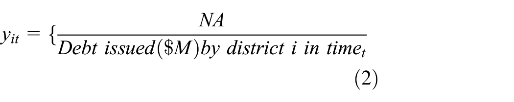
Debt issuance for district i in fiscal year t is defined as:

z_{it} = {\frac{1, if new debt > 0 for district i in time t}{0, otherwise}

(1)

and the amount issued is defined as:

y_{it} = {\frac{NA}{Debt issued ($ M) by district i in tim e_{t}}

(2)

The resultant model has two likelihoods, a Bernoulli distribution ( $z_{it} ~ Binomial (π_{it}, n_{it} = 1$ ) and a gamma distribution. ( $y_{it} ~ Gamma (a_{it}, b_{it})$ ). The gamma distribution is defined on a logarithmic scale, such that:

\log (y_{it}) = α_{i}^{y} + β_{itd}^{y} X_{itd} + τ_{t} + ϵ_{it}

(3)

where $α_{i}^{y}$ is a modelled intercept for district i, $β_{itd}$ represents a vector of parameters for time-varying district characteristics 1 to d and $ϵ_{it}$ represents the error term district i in time t. Further, $τ_{t}$ is a random effect for each fiscal year. Because $α_{i}$ nests yearly district observations by district ( $α_{i} = α_{0} + γ_{iv} W_{iv} + λ_{i}$ ) and $τ_{t}$ nests yearly district observations by year ( $τ_{t} = τ_{0} + ρ_{t}$ ), this is a cross-classified multilevel model. Each district-specific intercept is itself modelled as a function of time-invariant district variables 1 to v, such as district type, primary water source and whether the system purchases or sources its own water. A similar formulation is used to estimate the probability of any debt issuance, such that:

logit (π_{it}) = α_{i}^{z} + β_{itd}^{z} X_{itd} + τ_{t} + ϵ_{it}

(4)

where a separate set of parameters is estimated for the binomial model.

This two-stage approach is important given the conceptual aims of this article: the amount of debt issued is of less theoretical interest in this case since this amount is expected to be driven largely by basic district characteristics such as size and the number of households served. Modelling the decision to issue separately from the amount issued allows us to focus on the ability of districts to access debt financing as a capital investment tool, regardless of the issue size.¹¹

Data

In this study, we focus specifically on special purpose water districts identified as community water system operators in the US EPA Safe Drinking Water Act Information System (SDWIS). The practical advantage of focusing on these entities is that we are able to match SDWIS records to financial data obtained from the Texas Bond Review Board (TBRB) and institutional data from the Texas Water District Database (TWDD). Our working sample contains a total of 527 public service water districts (MUDs, FWSDs or WCIDs) active between 2008 and 2016 providing drinking water to residential communities.¹²

Violations data

We group violations into two primary categories: (1) health violations, which occur when the water supply contains contaminants in excess of regulatory limits or mandatory treatment techniques are not implemented; and (2) management violations, which occur when water systems neglect to follow monitoring and reporting requirements. Even health violations that are remedied by current resources might still motivate capital investment in order to prevent future violations or develop a more permanent solution. Thus, we use a lagged temporal window of health violations, contrasting systems that have experienced at least one major violation in the past three years with systems that have not. In other words, we use a binary indicator that represents whether a system has experienced a major violation within the three-year window. Accordingly, SDWA compliance data are obtained from 2005 to 2016 to allow for lagged observations from 2008 to 2016. This three-year window matches with the current time frame that EPA provides for each water system in the public SWDIS database, indicating that this three-year window is a policy-relevant frame.¹³ The number of systems thereby coded as violators ranges by year from 3% to 5%, while the proportion of management violators ranges from 8% to 35%.

Debt issuance data

Tax-exempt debt data for 2008–2016 are obtained from the TBRB and matched to the SDWA compliance data. We sum general-obligation (tax-based) debt and revenue-backed debt issued by each provider to generate total debt issued each year.¹⁴ The percentage of districts issuing new debt (i.e. excluding debt refinancing) in a given year ranges between 19% and 24%. The distribution of debt amounts issued is positively skewed, with median debt issue amount (amongst issuers) ranging between US$2.9m and US$10m across sample years, and mean issuance amount ranging from US$4m to US$12.8m.

Covariates

To incorporate other key drivers of investment, we model service pressure, district characteristics, economic characteristics and fiscal capacity. First, in general, older systems are anticipated to require more investment in order to achieve compliance. For a given year, we record the age of a system by subtracting the founding year (recorded in the TWDD) from the current fiscal year. Next, we follow Teodoro and Switzer (2016) in using two indicators of supply characteristics: whether the water system purchases water from another entity and whether a water system supplies groundwater. A district’s water source can affect storage, transfer and treatment facilities. Monitoring of groundwater requires monitoring at each extraction point (Levin et al., 2002). Moreover, land subsidence due to groundwater over-extraction in the region has prompted restrictions on groundwater withdrawal (Larson and Dziuk, 1995). Lastly, to account for the differential size and scale on which different systems operate, we also control for the number of household units that each district serves.¹⁵

Economic capacity is based on census tract median home values from the US American Community Survey (ACS). To generate district-level median home value estimates, we use GIS data to calculate the overlap of water districts on census tracts, and then compute a weighted average for each district based upon the extent of overlap. While median home values have a very strong correlation to other potential economic capacity indicators such as per capita income and poverty rates, we use the measure of median home value because it more closely reflects the tax base upon which each district can draw.

Finally, fiscal data for 2008–2016 for each public water system are obtained from annual audits filed within the TWDD.¹⁶ The primary variables of interest obtained from each annual audit are total revenue (combining tax revenue and service delivery fees) and total fund balance (combined balance in both general and enterprise funds). We use lagged total revenues as a proxy for fiscal capacity. To account for the impact of fund fiscal slack, we use lagged total fund balances for each special water district (by aggregating fund balances for general and enterprise funds). The term fund balance is used to represent the difference between current assets and liabilities even though we recognise that transactions are recorded using alternative accounting systems. We believe that both fund balance and net assets represent a reasonable proxy for fiscal slack. We further control for lagged outstanding debt to account for the conditioning role of existing bonded liabilities on new capital financing capacities. Table 1 provides descriptive statistics for model variables, as well as the source of each measure.

Table 1.

Descriptive statistics for model variables (last year observed).

	Min.	Median	Mean	Max.	Data source
Household equivalents ^a	8	1364	1839	94,390	TWDD^b
Med. home value	US$49,420	US$157,500	US$167,900	US$834,500	ACS^c
District age (years)	2.15	34.41	32.38	78.14	TWDD
Outstanding debt	US$ 0.00	US$10.64M	US$18.23M	US$217.80M	TBRB^d
Revenue_t-1 ^e	US$4.00	US$1.47M	US$1.77M	US$13.36M	TWDD
Fund balance_t-1 ^f	US$(-2.83M)	US$1.44N	US$1.92M	US$50.16M	TWDD
New debt	$ 0.00	$ 0.00	$1.02M	$41.21M	TBRB
Water type	72% groundwater		28% surface water		SDWIS^g
Procurement method	45% purchased		55% self-sourced		SDWIS
District type	478 MUD	35 WCID		14 FWSD	TWDD

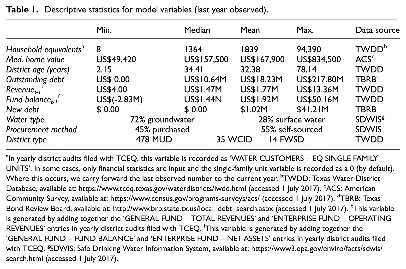
In yearly district audits filed with TCEQ, this variable is recorded as ‘WATER CUSTOMERS – EQ SINGLE FAMILY UNITS’. In some cases, only financial statistics are input and the single-family unit variable is recorded as a 0 (by default). Where this occurs, we carry forward the last observed number to the current year. ^bTWDD: Texas Water District Database, available at: https://www.tceq.texas.gov/waterdistricts/iwdd.html (accessed 1 July 2017). ^cACS: American Community Survey, available at: https://www.census.gov/programs-surveys/acs/ (accessed 1 July 2017). ^dTBRB: Texas Bond Review Board, available at: http://www.brb.state.tx.us/local_debt_search.aspx (accessed 1 July 2017). ^eThis variable is generated by adding together the ‘GENERAL FUND – TOTAL REVENUES’ and ‘ENTERPRISE FUND – OPERATING REVENUES’ entries in yearly district audits filed with TCEQ. ^fThis variable is generated by adding together the ‘GENERAL FUND – FUND BALANCE’ and ‘ENTERPRISE FUND – NET ASSETS’ entries in yearly district audits filed with TCEQ. ^gSDWIS: Safe Drinking Water Information System, available at: https://www3.epa.gov/enviro/facts/sdwis/search.html (accessed 1 July 2017).

Results

This analysis uses hierarchical Bayesian regression modelling. A Bayesian model estimates a posterior distribution for each parameter on the basis of a prior distribution¹⁷ and the modelled data (Gelman et al., 2013).¹⁸ This posterior distribution reflects our level of uncertainty about each parameter by presenting a probabilistic representation of the most likely parameter value given the observed data. We extract the 0.025 and 0.975 quantiles from each posterior distribution to produce 95% credible intervals. Credible intervals provide a straightforward interpretation: the estimated probability that the true parameter estimate lies between the upper and lower interval bounds is 95%. Each hypothesis is tested by determining whether the 95% credible interval includes zero.

Figure 1 presents full model results for all fixed parameters except for the intercept term. Tabular results for these models are presented in Appendix A. The upper (dark) intervals show the predicted additive change in the log odds of debt issuance given a one-unit change in the explanatory variable. Negative estimates represent a predicted decrease in the odds of debt issuance, while positive estimates increase these odds. The lower (light) intervals show the predicted change (on the additive log scale) in the amount of capital financing issued given debt issuance. Each parameter estimate is on the additive log scale (i.e. 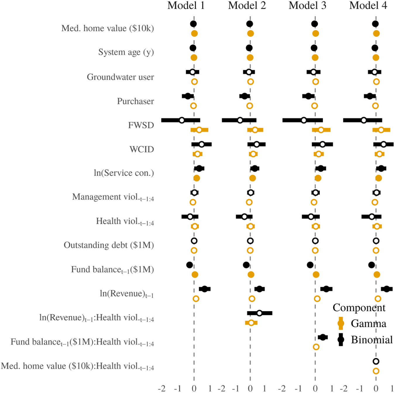$y_{it} = \log (α_{i}^{y} + β_{itd}^{y} X_{itd} + τ_{t} + ϵ_{it})$ ). Again, this means that negative estimates predict a lower level of new capital financing and positive estimates predict a higher level of new capital financing.

Figure 1.

Ninety-five percent credible intervals for water system debt issuance, binomial (debt issuance)-gamma (issuance amount) joint likelihood model.

Figure 1 presents four models. The first model contains no interaction terms. Models 2, 3 and 4 interact health violation occurrence with our two fiscal capacity indicators (revenue and fund balance) and one economic capacity indicator (median home value). For fiscal capacity measures, we use the natural logarithm of total revenue from taxes and service fees in the prior fiscal year and fund balance (untransformed, but scaled into US$ millions) in the prior fiscal year. For economic capacity measures in each water district, we focus on median home values (scaled into US$10k units).¹⁹ Each continuous covariate is mean centred, such that we observe predicted differences in log odds (of debt issuance) or additive log dollars (the size of debt issued) for violators at average covariate levels.

Our hypotheses primarily relate to the binomial, debt issuance portion of each semi-continuous model in Figure 1. The amount of debt issued (gamma likelihood) is expected to be more directly attributable to district size and scale. In Figure 1, higher median home values are associated with higher debt issuance amounts, and systems with more service connections are significantly more likely both to issue new debt and to issue increased amounts of debt. System age is negatively associated with the use of debt financing, but older systems that do issue debt are predicted to take out larger lines of credit. Further, as discussed previously, management violations are procedural in nature and not directly resolvable with capital investment. Thus, the null findings with respect to the impact of management violations on debt issuance and amount issued are in keeping with expectations.

While hypothesis 1 holds that the districts with higher fiscal capacity are more likely to use capital financing, Model 1 paints a slightly more nuanced picture. Namely, while high revenue districts are much more likely to issue new debt, districts with high fiscal slack (measured as fund balance) are less likely to use capital financing. The second portion of the model offers a potential explanation. High fiscal slack districts that do enter the credit market are associated with higher debt issuances on average. In other words, districts with a greater amount of funds on hand are less likely to use capital financing in general but tend to issue larger bonds when financing is used. We speculate that this is because districts with more fiscal slack can handle smaller maintenance and construction tasks without using the bond market. Conversely, districts with low fiscal slack on hand need credit to make small and large investments alike. Finally, economic capacity, as proxied by median home value, has a negative relationship (albeit small in magnitude) with the odds of capital financing. As noted above, median home value has a positive relationship with the amount of debt issued.

Turning to hypothesis 2, health violations are modelled with a binary indicator²⁰ of whether a system experienced one or more violations within the prior three years.²¹ In Model 1 we do not observe a positive relationship between prior health violation occurrence and subsequent new debt issuance. In fact, the estimated relationship is negative (although the credible interval does span zero). The extant literature shows that poorer neighbourhoods, particularly those with disadvantaged populations, have worse water services (Teodoro and Switzer, 2016). Thus, while we operationalise health violations as an indicator of service need, health violations themselves are potentially an indication of low capacity (and thus a lower probability of accessing capital financing).

In any case, Models 2, 3 and 4 in Figure 1 help to contextualise this result. Models 2 and 3 interact health violation occurrence with fiscal capacity (revenue and fund balance, respectively), while Model 4 interacts health violation occurrence with median home values, an indicator of economic capacity. Hypothesis 3 holds that the predicted impact of health violations on capital financing will be conditional upon fiscal and economic capacity levels. That is, response to a violation depends on the ability to pay. In evaluating hypothesis 3, we focus on the binomial portion of the model (predicting whether or not a system issues any debt).

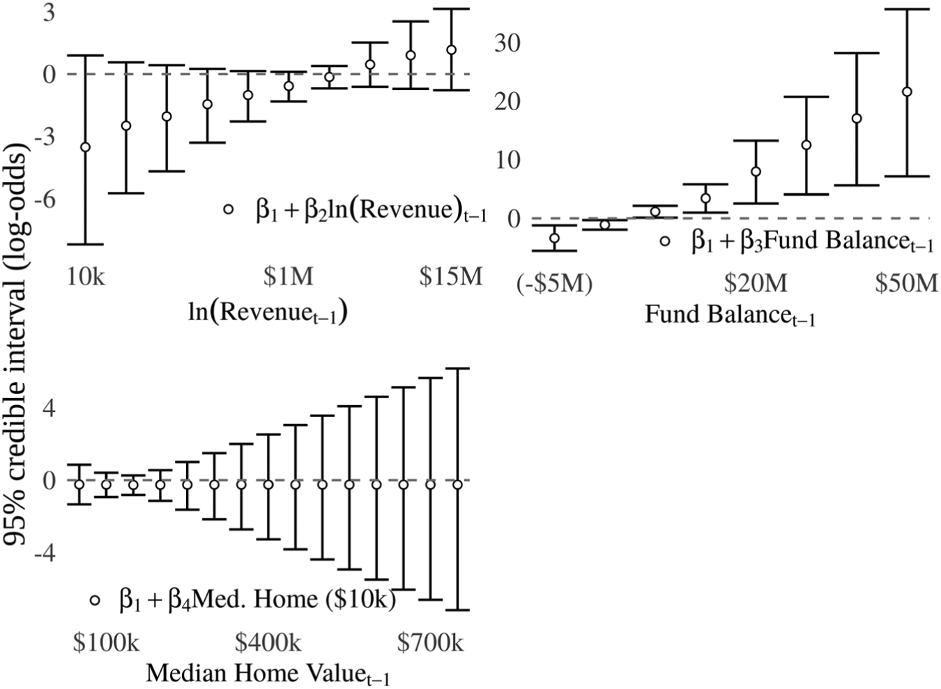
In order to test the interaction of health violations and each capacity indicator, we estimate linear combinations of the binary health violation variable and the interaction term (e.g. $β_{1} + β_{2} \ln (Revenu e_{t - 1})$ ). First, we compute a series of estimates across a range of values, and then derive the sampling variance for each combination (Martins et al., 2013). The resulting credible intervals for each combination are presented in Figure 2.

Figure 2.

Estimated 95% credible intervals for predicted marginal change in log-odds of debt issuance given a health violation at different capacity levels (based upon interaction terms in Models 2, 3 and 4).

The upper left panel in Figure 2 shows the predicted impact of health violations on new debt issuance. Note that because revenue is log-transformed, the scale of the x-axis in this panel is exponential. In any case, while the credible intervals for the range of linear combinations do span zero, there is nonetheless an upward trend, as districts with below-average revenue (below US$1.75M) are less likely to issue debt following a health violation and districts with above average revenue are more likely to do so post-violation. Since the total revenue variable is mean centred, an average district is not necessarily predicted to seek new capital financing following health violation occurrence. Only districts with above-average total revenue levels are predicted to issue new debt following such violations, while districts with below-average total revenue levels experience the opposite.

Turning to the interaction of health violations and the second fiscal capacity indicator, fund balance (Model 3), the upper right panel of Figure 2 shows a more stark conditional effect. Districts with a major health violation in the past three years that have a near-zero or negative fund balance are less likely than a non-violating district to issue new debt, even though these districts are presumably more in need of investment. In contrast, violating districts with a large and positive fund balance are much more likely to seek new capital financing relative to districts that have remained in compliance. Combined with the sizable (but non-significant) trend of health violations conditional upon revenue, this lends support to the expectation of hypothesis 3 that whether or not districts respond to health violations with new investment is in part dependent upon their fiscal slack.

The lower left panel of Figure 2 depicts credible intervals for different linear combinations of health violations interacted with median home values within a district. In this case, we do not observe a meaningful trend upwards or downwards. In other words, economic capacity does not modulate the predicted impact of health violations on new debt issuance. In part, this is likely because fiscal capacity is a more proximate metric of investment capabilities. Economic capacity is attenuated by myriad factors, including allocation agreements with general purpose governments, rate structure and other general political and economic constraints, whereas revenue and fund balance – fiscal capacity measures – are direct measures of institutional resources.²²

Implications for research and practice

The results of this analysis speak directly to the implications that system capacity can have on the ability of water service providers to invest in needed maintenance and infrastructure. We show that after committing a health violation districts with low overall fiscal capacity are less likely to take out debt for water system investment than are non-violating districts. These results indicate that some special water districts may lack the capacity to respond to service delivery failures when action is most needed.

The fact that regulatory violations are only associated with capital financing by higher fiscal slack water districts is troublesome. As regulatory violations by themselves are not found to matter for incidences of new capital debt issuance, policy makers are advised to develop mechanisms to enhance the fiscal capacities of less affluent jurisdictions and to offer them the ability to improve service performance. Ji et al. (2016) offer recent evidence that intergovernmental aid is instrumental for local government sustainability. This should be a reason for expanding mechanisms such as the Texas DWSRF and EPAP programmes. Scale issues are also a driving factor in the recent discussion of consolidation (Galvan, 2006); mergers and consolidation are potential solutions to the production challenges faced by small-scale providers (Hansen, 2013; Lee and Braden, 2008).

Going forward, there are several important extensions to this research. First, while sufficient and reliable data are not available to analyse other water providers in Houston, a broader focus on the full range of providers will speak more fully to key differences in capacity and service quality. Second, underlying water service provision is a vast exchange network. In order to better understand how – and whether – systems respond to violations, it is valuable to consider the regulatory behaviour and fiscal capacity of ‘upstream’ or ‘downstream’ districts. Thus, future work will draw upon water transfer records obtained from TCEQ to understand network patterns of water service delivery and performance. Finally, while wastewater and drinking water are governed under different regulatory structures, comparing and contrasting how water districts and other entities respond to Clean Water Act (CWA) violations versus SDWA violations could also shed more light on the regulatory behaviour of special water districts. In particular, some districts perform both functions, while others do not, providing a diverse set of institutional and service contexts to examine. By incorporating both of these regulatory regimes, future work can better explain the relationship between fiscal capacity and capital investment in response to regulatory violations.

Footnotes

Appendix A: Model results in tabular format

Table A1.

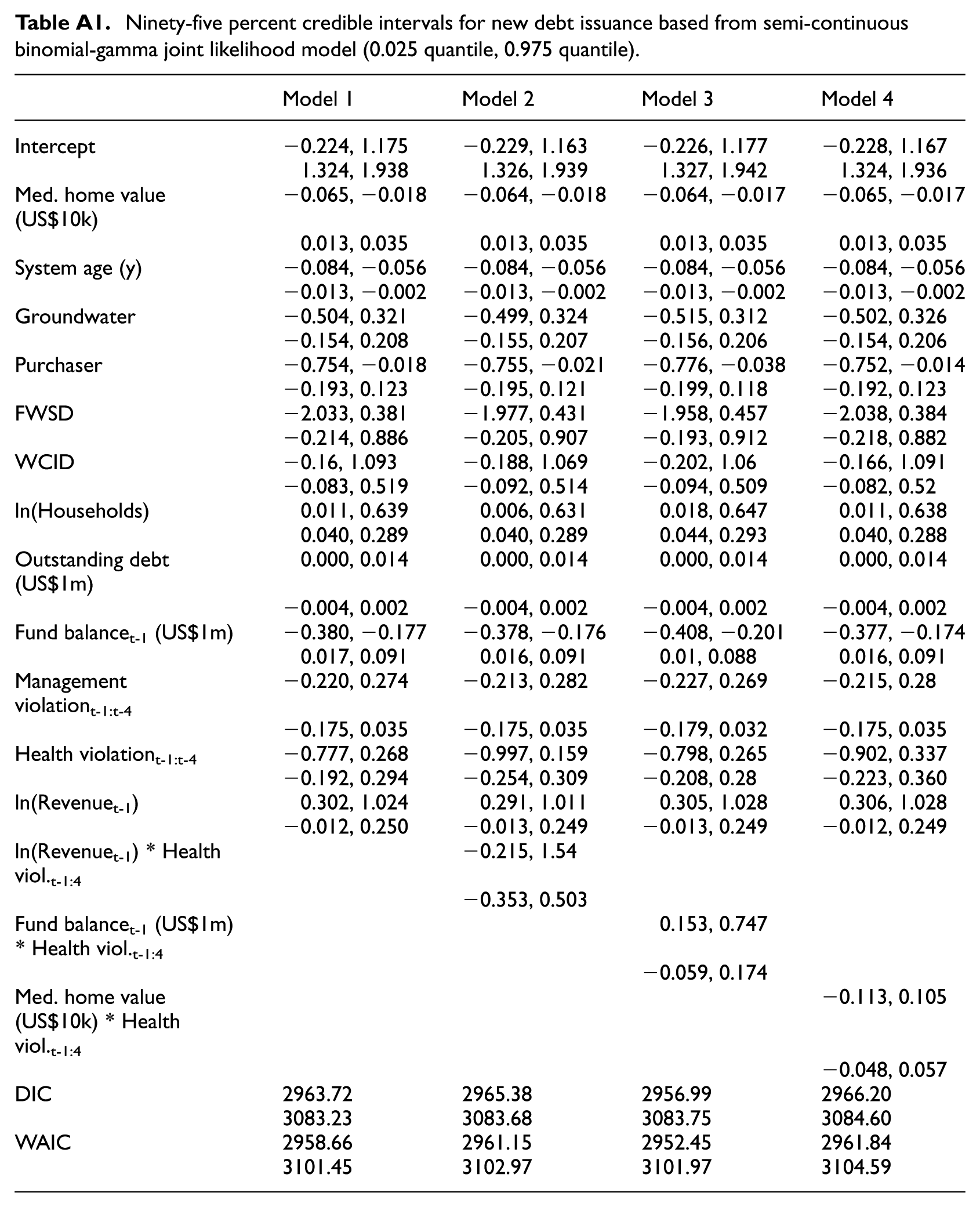
Ninety-five percent credible intervals for new debt issuance based from semi-continuous binomial-gamma joint likelihood model (0.025 quantile, 0.975 quantile).

	Model 1	Model 2	Model 3	Model 4
Intercept	−0.224, 1.175	−0.229, 1.163	−0.226, 1.177	−0.228, 1.167
	1.324, 1.938	1.326, 1.939	1.327, 1.942	1.324, 1.936
Med. home value (US$10k)	−0.065, −0.018	−0.064, −0.018	−0.064, −0.017	−0.065, −0.017
	0.013, 0.035	0.013, 0.035	0.013, 0.035	0.013, 0.035
System age (y)	−0.084, −0.056	−0.084, −0.056	−0.084, −0.056	−0.084, −0.056
	−0.013, −0.002	−0.013, −0.002	−0.013, −0.002	−0.013, −0.002
Groundwater	−0.504, 0.321	−0.499, 0.324	−0.515, 0.312	−0.502, 0.326
	−0.154, 0.208	−0.155, 0.207	−0.156, 0.206	−0.154, 0.206
Purchaser	−0.754, −0.018	−0.755, −0.021	−0.776, −0.038	−0.752, −0.014
	−0.193, 0.123	−0.195, 0.121	−0.199, 0.118	−0.192, 0.123
FWSD	−2.033, 0.381	−1.977, 0.431	−1.958, 0.457	−2.038, 0.384
	−0.214, 0.886	−0.205, 0.907	−0.193, 0.912	−0.218, 0.882
WCID	−0.16, 1.093	−0.188, 1.069	−0.202, 1.06	−0.166, 1.091
	−0.083, 0.519	−0.092, 0.514	−0.094, 0.509	−0.082, 0.52
ln(Households)	0.011, 0.639	0.006, 0.631	0.018, 0.647	0.011, 0.638
	0.040, 0.289	0.040, 0.289	0.044, 0.293	0.040, 0.288
Outstanding debt (US$1m)	0.000, 0.014	0.000, 0.014	0.000, 0.014	0.000, 0.014
	−0.004, 0.002	−0.004, 0.002	−0.004, 0.002	−0.004, 0.002
Fund balance_t-1 (US$1m)	−0.380, −0.177	−0.378, −0.176	−0.408, −0.201	−0.377, −0.174
	0.017, 0.091	0.016, 0.091	0.01, 0.088	0.016, 0.091
Management violation_t-1:t-4	−0.220, 0.274	−0.213, 0.282	−0.227, 0.269	−0.215, 0.28
	−0.175, 0.035	−0.175, 0.035	−0.179, 0.032	−0.175, 0.035
Health violation_t-1:t-4	−0.777, 0.268	−0.997, 0.159	−0.798, 0.265	−0.902, 0.337
	−0.192, 0.294	−0.254, 0.309	−0.208, 0.28	−0.223, 0.360
ln(Revenue_t-1)	0.302, 1.024	0.291, 1.011	0.305, 1.028	0.306, 1.028
	−0.012, 0.250	−0.013, 0.249	−0.013, 0.249	−0.012, 0.249
ln(Revenue_t-1) * Health viol._t-1:4		−0.215, 1.54
		−0.353, 0.503
Fund balance_t-1 (US$1m) * Health viol._t-1:4			0.153, 0.747
			−0.059, 0.174
Med. home value (US$10k) * Health viol._t-1:4				−0.113, 0.105
				−0.048, 0.057
DIC	2963.72	2965.38	2956.99	2966.20
	3083.23	3083.68	3083.75	3084.60
WAIC	2958.66	2961.15	2952.45	2961.84
	3101.45	3102.97	3101.97	3104.59

Declaration of conflicting interests

The author(s) declared no potential conflicts of interest with respect to the research, authorship, and/or publication of this article.

Funding

The author(s) received no financial support for the research, authorship, and/or publication of this article.

Notes

References

Blangiardo

Cameletti

(2015) Spatial and Spatio-Temporal Bayesian Models with R-INLA. Hoboken, NJ: Wiley.

Chen

Myles

Picot

(2011) Why have poorer neighbourhoods stagnated economically while the richer have flourished? Neighbourhood income inequality in Canadian cities. Urban Studies 49(4): 877–896.

Downey

(2007) US metropolitan-area variation in environmental inequality outcomes. Urban Studies 44(5–6): 953–977.

EPA Office of Water (2004) Variances and exemptions: A quick reference guide. Available at: https://nepis.epa.gov/Exe/ZyPDF.cgi?Dockey=901U0I00.txt (accessed 1 July 2017).

Galvan

(2006) Wrestling with MUDs to pin down the truth about special districts. Fordham Law Review 75: 341–380.

Gelman

Carlin

Stern

et al . (2013) Bayesian Data Analysis. Boca Raton, FL: CRC Press.

Greer

(2014) Overlapping local government debt and the fiscal common. Public Finance Review 43(6): 762–785.

Hansen

(2013) Estimating stakeholder benefits of community water system regionalization. Journal of the American Water Resources Association 105(10): 561–567.

Hildreth

Miller

(2002) Debt and the local economy: Problems in benchmarking local government debt affordability. Public Budgeting and Finance 22(4): 99–113.

10.

Hooghe

Marks

(2003) Unraveling the central state, but how? Types of multi-level governance. The American Political Science Review 97(02): 233–243.

11.

Ahn

Chapman

(2016) The role of intergovernmental aid in defining fiscal sustainability at the sub-national level. Urban Studies 53(14): 3063–3081.

12.

Jimenez

(2014) Separate, unequal, and ignored? Interjurisdictional competition and the budgetary choices of poor and affluent municipalities. Public Administration Review 74(2): 246–257.

13.

Jimenez

(2015) The fiscal performance of overlapping local governments. Public Finance Review 43(5): 606–635.

14.

Jimenez

Hendrick

(2010) Is government consolidation the answer?State and Local Government Review 42(3): 258–270.

15.

Johnson

Luby

Moldogaziev

(2014) State and Local Financial Instruments: Policy Changes and Management. Northampton, MA: Edward Elgar.

16.

Karuppusamy

Carr

(2012) Interjurisdictional competition and local public finance: Assessing the modifying effects of institutional incentives and fiscal constraints. Urban Studies 49(7): 1549–1569.

17.

Konisky

Teodoro

(2016) When governments regulate governments. American Journal of Political Science 60(3): 559–574.

18.

Larson

Dziuk

(1995) Groundwater to surface water conversion in the Houston-Galveston region: Impact of mandates on water quality, subsidence, and water rates. Risk Analysis 15(5): 545–554.

19.

Lee

MYA

Braden

(2008) Examining mergers in small CWSs: The role of regulatory compliance. Journal of the American Water Resources Association 100(11): 58–67.

20.

Levin

Epstein

Ford

et al . (2002) U.S. drinking water challenges in the twenty-first century. Environmental Health Perspectives 110(Suppl. 1): 43–52.

21.

Marlowe

(2005) Fiscal slack and counter-cyclical expenditure stabilization: A first look at the local level. Public Budgeting and Finance 25(3): 48–72.

22.

Martins

Simpson

Lindgren

et al . (2013) Bayesian computing with INLA: New features. Computational Statistics & Data Analysis 67: 68–83.

23.

Meyer

Konisky

(2007) Adopting local environmental institutions: Environmental need and economic constraints. Political Research Quarterly 60(1): 3–16.

24.

Mullin

(2009) Governing the Tap: Special District Governance and the New Local Politics of Water. Cambridge, MA: MIT Press.

25.

Mullin

(2010) Special districts versus contracts: Complements or substitutes. In: Feiock

Scholz

(eds) Self-Organizing Federalism: Collaborative Mechanisms to Mitigate Institutional Collective Action Dilemmas. New York: Cambridge University Press, pp. 142–160.

26.

Parks

Oakerson

(2000) Regionalism, localism, and metropolitan governance: Suggestions from the research program on local public economies. State and Local Government Review 32(3): 169–179.

27.

Rubin

(2013) Evaluating violations of drinking water regulations. Journal of the American Water Resources Association 105(3): 137–147.

28.

Rue

Martino

Chopin

(2009) Approximate Bayesian inference for latent Gaussian models by using integrated nested Laplace approximations. Journal of the Royal Statistical Society. Series B, Statistical Methodology 71(2): 319–392.

29.

Simonsen

Robbins

Helgerson

(2001) The influence of jurisdiction size and sale type on municipal bond interest rates: An empirical analysis. Public Administration Review 61(6): 709–717.

30.

Teernstra

(1993) How will small water systems finance SDWA compliance?Journal of the American Water Resources Association 85(6): 43–46.

31.

Teodoro

(2005) Measuring fairness: Assessing the equity of municipal water rates. Journal of the American Water Resources Association 97(4): 111–124.

32.

Teodoro

Switzer

(2016) Drinking from the talent pool: A resource endowment theory of human capital and agency performance. Public Administration Review 76(4): 564–575.