
Abstract
In 2016, Auckland implemented a widespread upzoning to encourage medium density infill housing. This article describes the institutional processes preceding the reform, quantifies the changes in land use across the metropolitan area and documents subsequent changes in residential housing starts. We show that approximately three-quarters of residential land was upzoned, predominantly in areas close to transportation network access, and between 5 and 25 km of the central business district (CBD). Six years on from the reform, housing starts have increased; are located closer to the CBD, employment locations and transportation network access points; and are predominantly infill and attached housing. Spatial decompositions show that these patterns are exclusively driven by changes in housing starts in upzoned areas.
Introduction
Zoning reform is increasingly being advocated to achieve a variety of urban policy goals, such as increasing housing supply and reducing housing costs (Freeman and Schuetz, 2017; Glaeser and Gyourko, 2005), reducing spatial inequities (Manville et al., 2020) and enabling a more compact and environmentally sustainable form of urban development (Wegmann, 2020). There remains, however, little empirical evidence on the impacts of large-scale zoning reforms on housing supply and costs (Freeman and Schuetz, 2017; Schill, 2005), let alone changes on urban development patterns or spatial inequality, in part because reforms of a scale sufficient to have a substantial impact on metropolitan development patterns are scarce (Freeman and Schuetz, 2017).
However, in 2016 the city of Auckland, New Zealand, upzoned a substantial amount of its residential land under the Auckland Unitary Plan (AUP). Consents for new dwellings subsequently reached record highs, in both absolute and per capita terms, and the city’s consenting rate has increased from one of the lowest in the Australasian region to the highest (Greenaway-McGrevy, 2023). Auckland therefore provides a unique and important case study for the design and implementation of widespread zoning reform.
This article provides a narrative of the events preceding and following the reform. First, we describe the institutional context underlying the AUP, the goals of the reform and the process of implementation. Governance changes and centralisation of decision-making featured prominently in strategy and implementation. Second, we quantify the scale of the reform by estimating the amount of upzoned land, both across the city and in relation to key amenities. Using a geocoded dataset of land parcels matched to planning zones, we show that the maximum floor-to-area ratio (FAR) was relaxed on approximately three-quarters of residential land, with much of this upzoning occurring between 5 and 25 km of the CBD, and in close proximity to transportation networks and areas of concentrated employment. Finally, we examine whether subsequent changes in housing development accord with the reform’s goals, which included increasing housing supply and geographically contracting urban growth. To do this, we present a conceptual framework where zoning reform increases the housing stock via an increase in housing supply in upzoned areas.
We test this prediction using an empirical model that compares changes in housing starts in upzoned areas to changes in non-upzoned areas subsequent to the reform. We fit the model to a geocoded dataset of new dwelling consents (‘building permits’ in the USA). We show that: housing starts in upzoned areas increased substantially relative to non-upzoned areas; the spatial distribution of consents has contracted towards the CBD, transportation network access points and employment locations; and the contraction is due exclusively to increases in consents in upzoned areas.
The effects of zoning reform on housing and urban development remain an important but regrettably understudied topic. A handful of studies that focus on localised (or ‘spot’) upzonings typically show muted or no effects. Freemark (2020) shows that transit-orientated upzoning in Chicago failed to stimulate construction, while Peng (2023) shows that housing supply responded slowly to a sequence of localised upzonings in New York. Dong (2024) finds that localised upzonings in Portland approximately doubled the long-term probability of parcel development, but the number of new units constructed remains small. In recent work, Stacy et al. (2023) show that various reforms in US cities between 2000 and 2019 generated negligible increases in housing supply, on average. In contrast, widespread zoning reforms are found to have larger effects in a couple of papers. Gray and Millsap (2023) show that the city-wide reduction in minimum lot sizes in Houston preceded an increased concentration of development activity in middle-income, less dense, under-built neighbourhoods, while Greenaway-McGrevy (2023) shows that the AUP precipitated a significant increase in housing starts. Our article complements the latter by detailing how the spatial distribution of land use and housing construction has changed, thereby demonstrating that the reform successfully encouraged a more spatially compact pattern of growth.
The remainder of the article is organised as follows. The section ‘Institutional background’ describes the institutional processes behind the AUP, including changes in local governance, its policy objectives and how its structure informs our empirical work. The section ‘Changes in residential land use’ documents geographical variation in regulatory changes under the plan. The section ‘Changes in housing development’ documents empirical changes in housing starts that are consistent with the goals of the reform. The section ‘Concluding remarks’ concludes by drawing lessons for policymakers considering similar large-scale zoning reform.
Institutional background
Auckland, the largest city in New Zealand, has had a rapidly growing population that increased from 1.16 to 1.57 million between 2001 and 2018 (source: census). Centred on a long isthmus between two harbours, it extends over 4894 km2 of land, including a large metropolitan area, several towns, populated islands and a substantial amount of rural land.
Until 2010, the region comprised seven city and district councils, each developing and implementing land use plans. The four city councils (Auckland, North Shore, Manukau and Waitākere) encompassed the developed areas in the suburbs around the CBD, and the former Auckland City Council covered the CBD and central isthmus. Two district councils (Rodney and Franklin) covered predominantly rural areas, while Papakura district council administered a formerly discontiguous town.
A critical antecedent to the zoning reform was the amalgamation of the seven councils to form a single jurisdiction (Auckland Council, ‘AC’) by an act of parliament in 2009 ( Local Government (Auckland Council) Act 2009 ). This centralised the formerly fragmented governance structure into a single ‘unitary’ authority with enhanced powers to plan the metropolis as a whole. Parliament also created statutory requirements for a strategic spatial plan and a consistent set of LURs for the region ( Local Government (Auckland Council) Amendment Act 2010 ; Local Government (Auckland Transitional Provisions) Act 2010 ).
AC released the spatial plan in 2012 (Auckland Council, n.d.). Motivated by sustainable development, it directed the majority of growth to occur within the existing urban area, setting a target of 60–70% of new dwellings within the 2010 ‘metropolitan urban limit’. AC then released consistent planning rules under the ‘draft’ AUP in March 2013, which included widespread relaxation of LURs to achieve the strategic goals set out in the spatial plan. After 11 weeks of public consultations, AC released a revised ‘Proposed’ AUP (PAUP) in September.
Prior to the notification of the PAUP, AC proposed that the central government appoint an independent hearings panel (IHP) to receive submissions and make recommended changes to the PAUP. The additional community engagement would substitute for limited appeal rights to IHP recommendations, thereby accelerating implementation by avoiding lengthy litigation (Blakeley, 2015). The government agreed and amended the facilitating legislation ( Local Government (Auckland Transitional Provisions) Amendment Act 2013 ).
The IHP received submissions between April 2014 and May 2016, and released recommended changes to the plan on 22 July 2016. A primary recommendation was the abolition of minimum lot sizes for existing parcels. AC considered and voted on the IHP recommendations over the next 20 working days. On 19 August 2016, AC released the ‘decisions’ version of the AUP, including new zoning maps. Several of the IHP’s recommendations were voted down, including the abolishment of minimum floor sizes on apartments. This was followed by a 20-day period for the public to lodge appeals in the Environment Court, while appeals to the High Court were only permitted if based on points of law. The ‘final’ version of the AUP became operational in part on 15 November 2016. 1
However, the AUP began to have limited effects upon notification of the PAUP in September 2013. The Auckland Housing Accord (AHA), an interim agreement between AC and the central government, allowed developers to build under the PAUP in exchange for affordable housing provisions (New Zealand Government, n.d.). This agreement modified a national inclusionary zoning programme called ‘Special Housing Areas’ (SpHA), also launched in September 2013, that offered developers an accelerated consenting process in exchange for a 10% affordable housing provision ( Housing Accords and Special Housing Areas Act 2013 ). The agreement expired upon operationalisation of the AUP. The total number of dwellings consented under the programme was comparatively small.
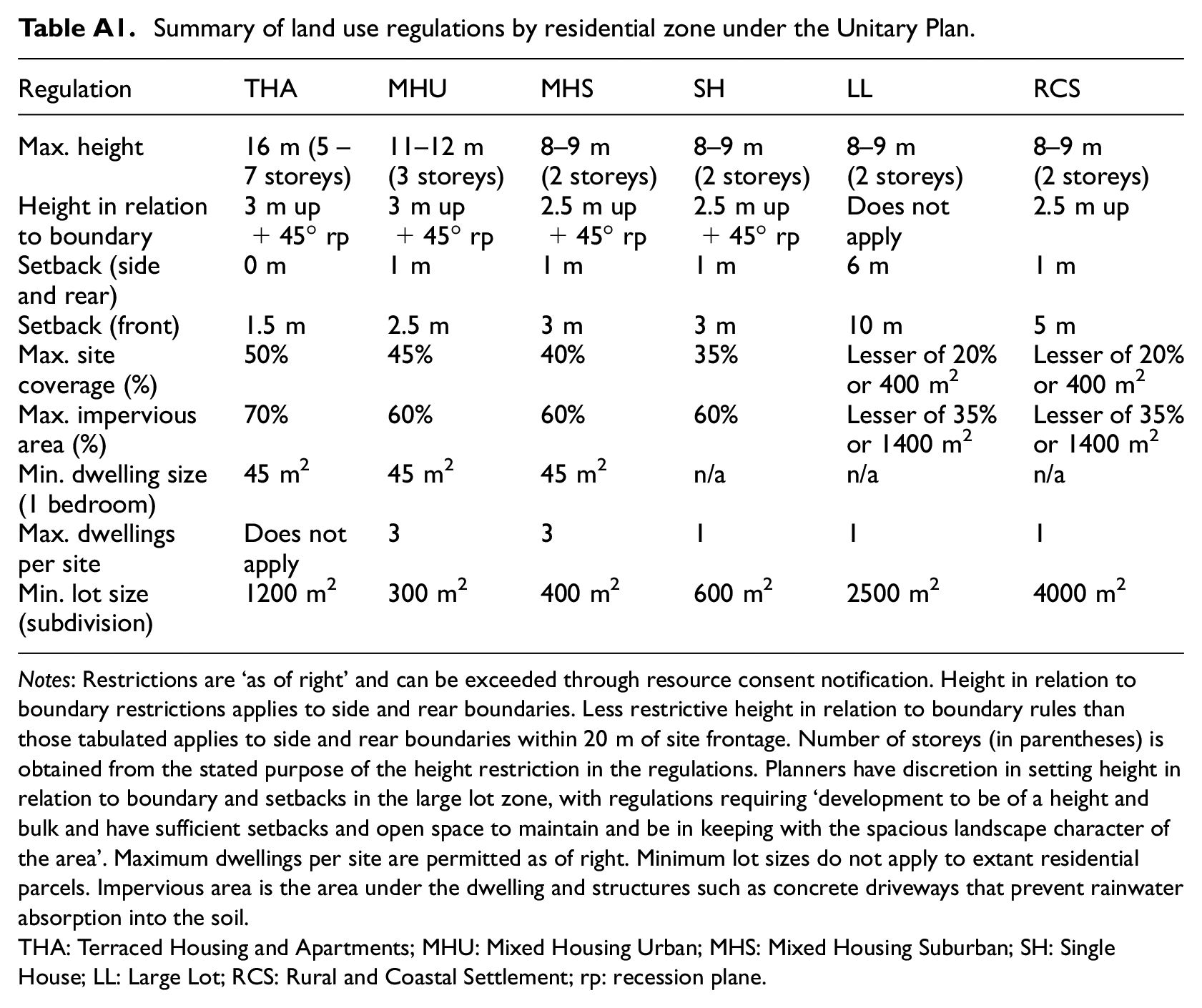
Each version of the AUP (‘draft’, ‘proposed’, ‘decisions’ and ‘final’) could be viewed online by the public and disclosed new LURs that would potentially change restrictions on permissible site development, depending on zoning. Four residential zones were introduced. Listed in decreasing order of permissible site development, these were: Terrace Housing and Apartments (THA), Mixed Housing Urban (MHU), Mixed Housing Suburban (MHS) and Single House (SH). Table A1 in the Appendix summarises various LURs for each zone, including SCRs, height restrictions, setbacks and recession planes. For example, five to seven storeys and a maximum SCR of 50% is permitted in THA, whereas two storeys and a coverage ratio of 35% is permitted in SH. Up to three dwellings per parcel is allowed in MHS and MHU. As we demonstrate below, the new LURs were more permissive than those of the pre-AUP plans in most residential areas. The AUP also includes two additional ‘residential’ zones for semi-rural areas –‘Large Lot’ and ‘Rural and Coastal Settlement’– that apply to peri-urban areas or small settlements distant to the CBD, often without water infrastructure. LURs in these zones restricted development to very low intensity, as shown in Table A1. We refer to these zones as ‘semi-rural’.
Changes in residential land use
We quantify the amount of land upzoned under the AUP by matching individual land parcels to GIS information on planning zones. The parcel data are as of November 2016, when the AUP became operational, and contain the geocoordinates of each parcel’s vertices, enabling calculation of land area, and matching to other spatial information. Each parcel is matched to its AUP and pre-AUP planning zones.
To determine whether a parcel was upzoned, we require a measure of the allowable capital intensity of housing under the AUP and previous regulations. While it is relatively straightforward to derive such a measure for the AUP zones, there were approximately 115 residential zones across the seven pre-AUP council plans, each with site coverage ratios (SCRs), height restrictions, minimum lot sizes per dwelling, setbacks and recession planes. We use the maximum FAR as the measure of LUR stringency. FARs are frequently used for this purpose (Brueckner and Singh, 2020; Brueckner et al., 2017; Tan et al., 2020). SCRs and height limits were near universal in all pre-AUP zones, meaning each zone’s FAR can be obtained by multiplying the SCR by the number of storeys implied by the height limit.2,3 The majority of the pre-AUP zones also had minimum lot size restrictions, which do not apply to extant parcels under the AUP.
We group the pre-AUP residential zones into categories based on their respective FARs (henceforth ‘zoning categories’). These categories accord with the maximum FAR permitted in the four AUP residential zones because we are interested in how LURs affecting individual parcels changed under the AUP. This enables us to identify upzoned parcels as parcels where LURs were relaxed. THA has a FAR of 2.5 under its five-storey and 50% SCR limits. We therefore define the ‘Residential-High’ category as zones with FARs no less than 2.5. MHU has a FAR of 1.35, and thus ‘Residential-Medium’ comprises zones with FARs greater than or equal to 1.35 and less than 2.5. MHS has a FAR of 0.8, and thus ‘Residential-Medium-Low’ comprises zones with FARs greater than or equal to 0.8 and less than 1.35. SH has a FAR of 0.7, and thus ‘Residential-Low’ comprises zones with FARs greater than or equal to 0.7 and less than 0.8. We include zones intended to preserve built or natural heritage as ‘Residential-Low’, unless applied to semi-rural areas. Finally, we define ‘Semi-Rural’ as having a FAR less than 0.7 but greater than or equal to 0.15.
We allocate each parcel to an AUP zone and a pre-AUP residential zone category. We include ‘business’ and ‘rural and open space’ categories in these allocations. We also have a ‘mixed’ category for a few pre-AUP ‘special area’ zones that allowed various housing forms within one contiguous area. The aggregate amount of land in each AUP zone can then be decomposed into the various pre-AUP zone categories, enabling us to observe changes in land use, and the amount of land that was upzoned.
Table 1 presents the amount of land allocated to the various pre-AUP categories and AUP zones. Prior to the AUP, 95.2% of residential land falls under the low-density category. The AUP enabled a significant increase in the amount of land allocated to medium- or high-intensity residential development. Prior to 2016, the total residential area with a FAR of 2.5 (equivalent to THA) or above (i.e. Residential-High) was less than half a square kilometre. The AUP introduced 25 km2 of THA that allows a FAR of 2.5. Similarly, prior to 2016, there was 4.04 (= 3.66+0.38) km2 of residential land that allowed a FAR of 1.35 (equivalent to MHU) or above. This increased to approximately 100 km2 (= 75.49+24.52) under the AUP.
Changes in land use (land area in km2).
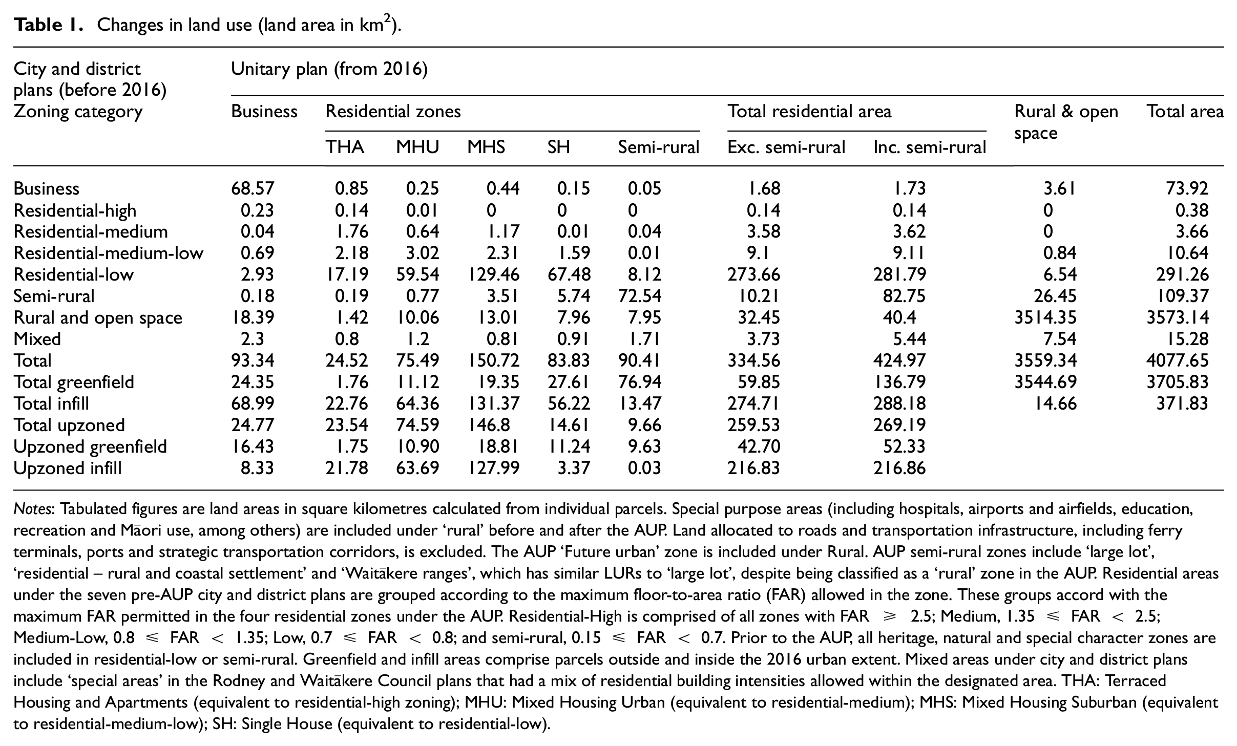
Notes: Tabulated figures are land areas in square kilometres calculated from individual parcels. Special purpose areas (including hospitals, airports and airfields, education, recreation and Māori use, among others) are included under ‘rural’ before and after the AUP. Land allocated to roads and transportation infrastructure, including ferry terminals, ports and strategic transportation corridors, is excluded. The AUP ‘Future urban’ zone is included under Rural. AUP semi-rural zones include ‘large lot’, ‘residential – rural and coastal settlement’ and ‘Waitākere ranges’, which has similar LURs to ‘large lot’, despite being classified as a ‘rural’ zone in the AUP. Residential areas under the seven pre-AUP city and district plans are grouped according to the maximum floor-to-area ratio (FAR) allowed in the zone. These groups accord with the maximum FAR permitted in the four residential zones under the AUP. Residential-High is comprised of all zones with FAR ≥ 2.5; Medium, 1.35 ≤ FAR < 2.5; Medium-Low, 0.8 ≤ FAR < 1.35; Low, 0.7 ≤ FAR < 0.8; and semi-rural, 0.15 ≤ FAR < 0.7. Prior to the AUP, all heritage, natural and special character zones are included in residential-low or semi-rural. Greenfield and infill areas comprise parcels outside and inside the 2016 urban extent. Mixed areas under city and district plans include ‘special areas’ in the Rodney and Waitākere Council plans that had a mix of residential building intensities allowed within the designated area. THA: Terraced Housing and Apartments (equivalent to residential-high zoning); MHU: Mixed Housing Urban (equivalent to residential-medium); MHS: Mixed Housing Suburban (equivalent to residential-medium-low); SH: Single House (equivalent to residential-low).
These increases in the amount of residential land under the high, medium and medium-low categories imply that many parcels were upzoned, because a shift to a higher-density zoning category entails a relaxation on LURs. Our analysis in the section ‘Changes in housing development’ requires the classification of parcels as either upzoned or non-upzoned. The final three rows of Table 1 display the total amount of residential land upzoned, including by greenfield and infill areas, where greenfield (infill) refers to parcels that lie outside (inside) of the urban extent as of 2016. 4
Upzoned land comprises: (i) all residential parcels that previously had a FAR below that of their AUP zone; (ii) all parcels zoned for residential in 2016 that were previously zoned rural or open space; and (iii) parcels zoned for business in 2016 that were previously zoned residential or rural. We also classify ‘mixed’ areas pre-AUP as upzoned. This choice makes little difference, given the small area of mixed land not re-zoned to rural under the AUP (7.74 km2).
Approximately 260 of the 335 km2 (or 77.6%) of residential land was upzoned. Looking at the four main residential AUP zones, 23.5 of the 24.5 km2 (or 95.9%) of THA was upzoned, with the majority – 17.2 km2– being rezoned from Residential-Low. Meanwhile, 74.6 of the 75.5 km2 (or 98.8%) of MHU was upzoned, again with the vast majority – 59.5 km2– from Residential-Low. Similarly, 146.8 of the 150.7 km2 (or 97.4%) of MHS was upzoned, 129.5 km2 of which came from Residential-Low. 5 In total, approximately 98% of land allocated to MHS, MHU or THA was upzoned. In contrast, most SH land was not upzoned, as it was previously classified as Residential-Low. Nonetheless, approximately 13.7 km2 of SH was previously classified as Rural or Semi-Rural, and thus was upzoned to SH. Approximately 71% (= 42.7/59.85) of greenfield residential land was upzoned, and 79% (= 216.83/274.71) of infill residential land.
Very little land was downzoned, in the sense that the parcel was in a more intensive residential category prior to 2016. For example, 0.26 km2 of MHU was classified as Residential-High or Business, while 1.61 km2 of MHS was classified as -High, -Medium or Business.
Figure 1 maps the upzoned residential areas, decomposed into upzoned to THA, MHU and MHS. For clarity, we focus exclusively on residential areas, omitting parcels upzoned to business or semi-rural. Non-upzoned residential areas comprise SH, MHS, MHU and THA zoned parcels that, prior to 2016, had a FAR greater or equal to that permitted under the AUP. The majority of this area consists of SH parcels that were not upzoned from semi-rural or rural.
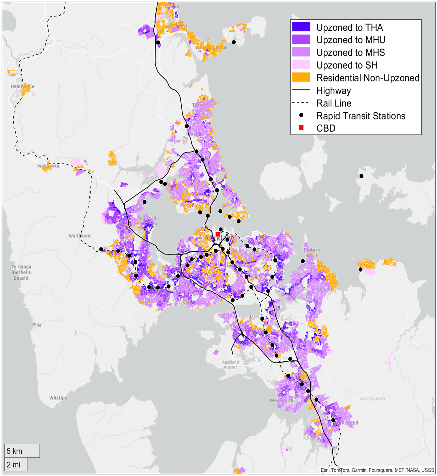
Upzoned and non-upzoned residential areas of Auckland.
Spatial distribution of upzoning
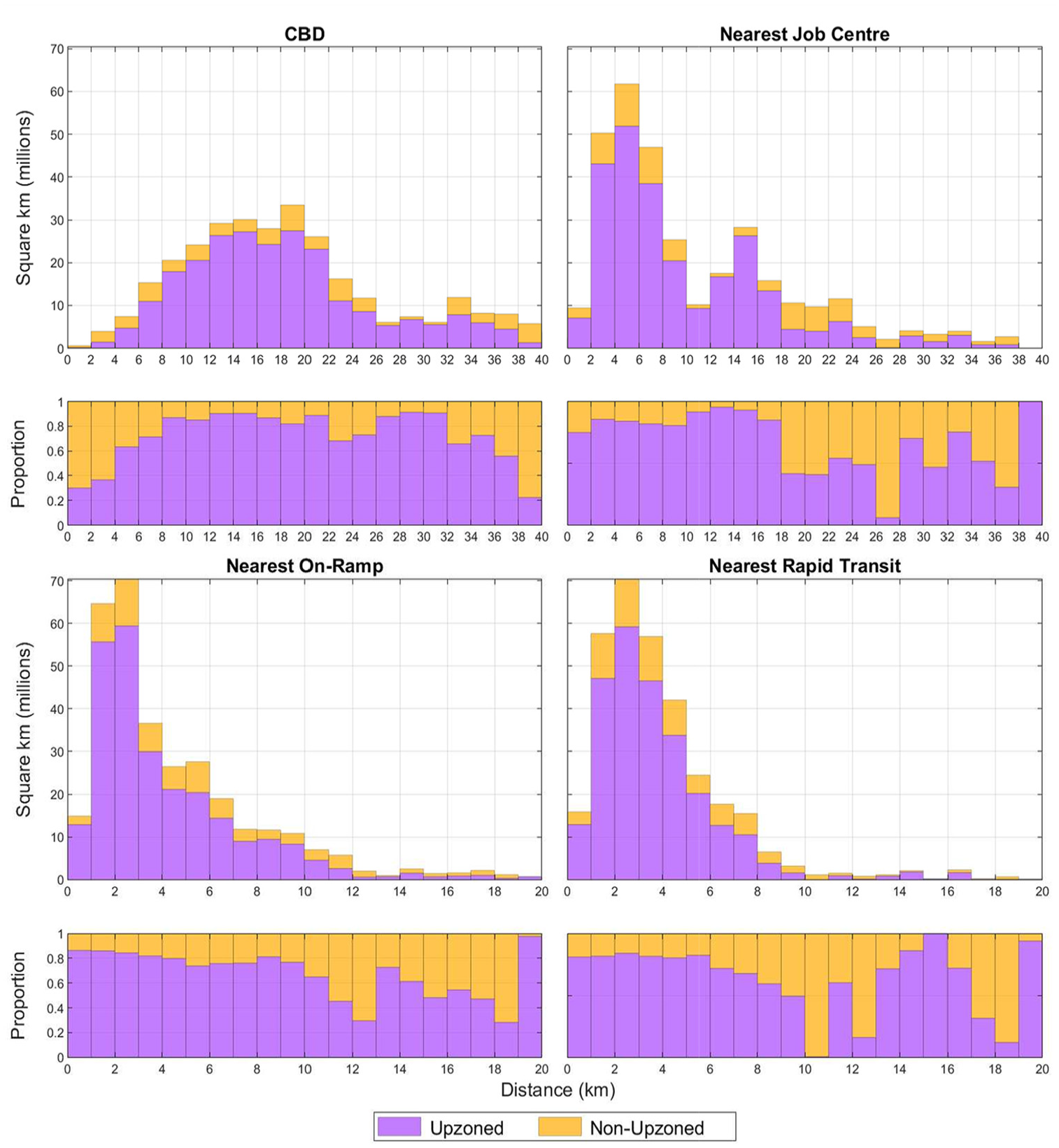
This section quantifies the amount of upzoned residential land relative to geographically fixed points that influence household locational choice. Specifically, we measure the amount and proportion of upzoned land at different distances to: the CBD; the nearest job centre; the nearest highway on-ramp; and the nearest rapid transit (RT) station. We use network distances (the shortest path on extant road networks) from the centroid of the meshblock in which the parcel is located. 6 Job centres are areas with a disproportionately high number of employees. 7
For each fixed point, we calculate the amount of non-upzoned and upzoned residential land within various distances. Figure 2 depicts the results, alongside the proportion of upzoned land. The Supplemental Material includes a figure that decomposes the upzoned areas by AUP zone.
Distance between upzoned land and locations of interest.
The bulk of residential land is between 5 and 25 km of the CBD. The upzoned proportion is highest between 5 and 35 km, consistently exceeding 60%. This reflects SH areas being predominantly located either close to the CBD, under ‘character’ neighbourhood protections, or far from the CBD. For example, within 2 km of the CBD, approximately 30% is upzoned, while between 2 and 4 km, less than 40% is upzoned. The majority of residential land is between 2 and 10 km from a job centre. The upzoned proportion is fairly constant, at approximately 80% or above, out to 18 km. The majority of residential land is within 1 – 6 km of a highway on-ramp or an RT station. The proportion of upzoned land is fairly uniform with respect to distance to on-ramps, whereas it decreases beyond 6 km from RT stations.
Changes in housing development
This section documents changes in housing development. We use a dataset of individual new building consents (hereafter ‘consents’) issued by AC and its predecessors. These are algorithmically matched to individual parcels by combining the consent’s geocoordinates and address (see the Supplemental Material for details). The matched data span 2000 – 2022.
Before proceeding, we note that consents reflect housing starts, not completed dwellings. Unfortunately, data collection and administration make it difficult to directly measure completions for dwellings consented prior to 2018. However, estimates from 2018 onwards suggest completion rates of over 90%, with higher rates in upzoned areas. Extensive details are provided in the Supplemental Material.
Conceptual framework
Our empirical analysis is motivated by economic frameworks that conceptualise zoning reform as increasing housing supply. To conserve space, we relegate the exposition of the model to the Supplemental Material, providing the intuition of the model here.
In theories of urban development such as Bertaud and Brueckner (2005), LURs place lower bounds on the amount of land required to build housing. Upzoning relaxes these minima. This reduction in input costs increases housing supply, shifting the supply curve out and generating an increase in housing, holding all else constant. 8
When there is geographical variation in upzoning, supply increases are greater in locations with larger increases in minimum constraints, since comparatively less land is required to produce housing in these areas (Greenaway-McGrevy, forthcoming). This observation informs our empirical strategy, as it implies that increases in aggregate metropolitan supply of housing are likely to be more manifest in the more permissive upzoned areas than in non-upzoned areas. We test this implication in the section ‘Consents’ using an empirical model that estimates differences in consents between upzoned and non-upzoned areas.
The increase in housing is moderated by housing demand, which varies by location under conventional models of urban development. In the canonical Alonso–Muth–Mills model, commuting time moderates demand. This principle can be generalised for access to other locational amenities. The straightforward corollary is that upzoning shifts the geographic distribution of housing construction towards desirable amenities, provided land close to these geographic features is upzoned. Again, the shift manifests in upzoned areas, and we empirically test this implication in the section ‘Consents’.
Consents are also affected by a variety of demand- and other supply-side factors. For example, exogenous reductions in interest rates, relaxation of mortgage lending criteria or increases in population would increase demand for housing, while an exogenous reduction in the cost of building materials or construction workers would generate an increase in supply. Less tangible changes, such as a more relaxed attitude towards development by local government, or improvements in the management and practice of housing construction, would also manifest as an increase in consents. However, because they plausibly affect residential construction regardless of zoning, these variables manifest as increases in both upzoned and non-upzoned areas – not the differential increase in upzoned areas relative to non-upzoned, as implied by our conceptual framework, and measured in our empirical models.
Consents
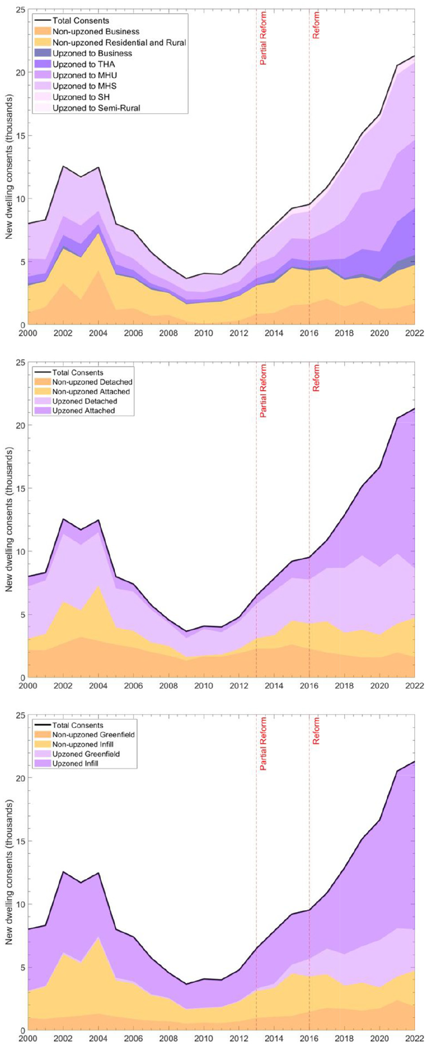
Figure 3 presents annual consents between 2000 and 2022 decomposed into different areas, including by zoning change. Total consents increase from approximately 9200 in 2015, the year prior to the AUP becoming operational in November 2016, to 21,000 by 2022, far exceeding the previous peak of 12,500 consents in 2002, which was driven by a construction boom in business areas (particularly the CBD). 9
Dwelling consents by 2016 zoning change, 2000 to 2022.
The top panel decomposes consents by zoning change. All of the increase since 2016 is in upzoned areas. In 2015, 4700 consents were issued in areas that would go on to be upzoned in 2016, while 4500 were issued in areas that would not. By 2022, 16,600 were issued in upzoned areas, while 4700 were issued in non-upzoned areas.
Most of the increase in consents since 2016 is due to increases in areas upzoned to MHS, MHU or THA. Of the 16,600 consents issued in upzoned areas in 2022, 15,300 were issued in one of these three areas.
Attached and detached housing
Upzoning is associated with attached housing structures, such as plexes, rowhouses and apartments, due to their more efficient use of space. The middle panel of Figure 3 decomposes consents into attached and detached dwellings. Most of the increase since 2016 is attached dwellings in upzoned areas.
Infill and greenfield development
A key strategic goal underpinning the zoning reform was to promote housing in existing urban areas. To examine this, we bifurcate the sample into greenfield and infill development. Following Biddle et al. (2006), we use ‘infill’ to refer to redevelopment or intensification of existing residential land, as well as residential construction on commercial zoned land.
We use the ‘urban extent’ of Auckland to delineate greenfield and infill housing development. The urban extent is a geographical measure of developed urban areas that excludes rural, peri-urban (i.e. semi-rural) and open space areas. It is constructed by AC using satellite imagery of cadastral land parcels. See the Supplemental Material for a graphical depiction and a resource describing the concept and classification methodology. We decompose the sample into parcels inside and outside the 2016 urban extent.
The bottom panel of Figure 3 shows that there have been increases inside and outside the urban extent. Most of the increase is due to upzoned areas within the urban extent (i.e. upzoned infill), although there has been an increase in upzoned greenfield development as well.
In the analysis to follow, we focus solely on residential areas (SH, MHS, MHU and THA), as the spatial plan underpinning the AUP was focused primarily on increasing density in residential areas, and most of the increase in dwelling consents is in upzoned residential areas, as shown in the top panel of Figure 3.
Empirical model
The relative increase in housing starts in upzoned areas compared to non-upzoned areas illustrated in Figure 3 is consistent with the predictions of our conceptual framework. However, the differential increase between upzoned and non-upzoned areas may reflect systematic differences in long-run trends between upzoned and non-upzoned parcels, rather than the policy change itself. For example, planners may have targeted desirable suburbs or parcels for upzoning, such that the increase in consents in upzoned areas reflects a supply response to increasing demand that would have occurred under the counterfactual of no upzoning. The differential increase could also be due to time variation in unobserved confounders occurring at the same time as the policy.
To address these potential pathologies, we fit the following regression to individual parcels:
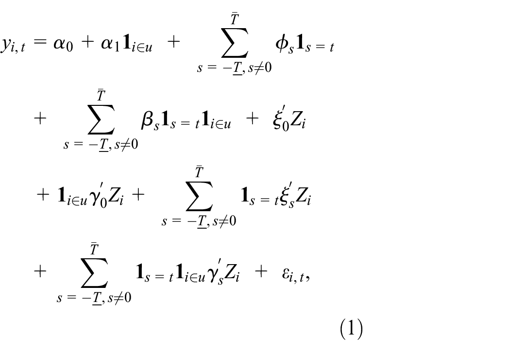
where
The sequence of coefficients
Meanwhile,
The period fixed effects
The model also includes parcel-level covariates in the vector
These covariates account for parcels selected for upzoning. These selection criteria may interact with variation in demand-side factors to generate changes in consents in upzoned areas that would otherwise be misattributed to the reform. For example, suppose that a significant increase in traffic congestion at the same time as the reform increased demand for housing close to transportation network access points, generating an increase in consents on upzoned parcels because such parcels are more likely to be close to on-ramps or RT stations. Confounders that are not included or approximated in the set of covariates will not be controlled for. For example, if, even after conditioning on these observable characteristics, areas or lands zoned for higher-density housing are more (or less) sensitive to the factors underlying construction cycles, then variation in these factors will manifest as differential construction rates between upzoned and non-upzoned parcels. However, such differentials would likely also manifest prior to upzoning, and thus be diagnosable.
Following the suggestion of Meyer (1995), the covariates have differential impacts in upzoned and non-upzoned areas. We provide evidence of this heterogeneity in the Supplemental Material to the article. We estimate models both with and without these covariates.
Figure 4 exhibits the estimates of
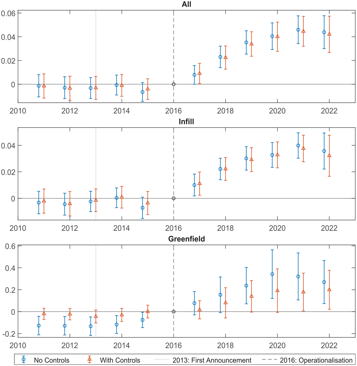
Difference in consents per parcel between upzoned and non-upzoned areas, 2011–2022.
After 2016, the coefficients trend upwards. For all consents, they reach 0.045 by 2022. This indicates that each upzoned parcel had 0.045 more consents issued (on average) than non-upzoned parcels in 2022. Unsurprisingly, upzoning has a much larger impact on the probability of greenfield development than infill. After conditioning on covariates, the increase in the probability of development reaches 0.19 by 2022.
Spatial distribution of consents
Next, we illustrate changes in the spatial distribution of consents relative to geographically fixed points. To do so, we calculate the network distance between the centroid of each consent’s meshblock and: the CBD; the nearest job centre; the nearest highway on-ramp; and the nearest RT station.
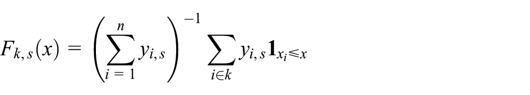
The top row of Figure 5 depicts the empirical (cumulative) distribution function (EDF) of the distance between consents and the various locations. The x-axis plots distance to the location. The EDF is then the proportion of consents that are within a given distance as measured on the x-axis. Let
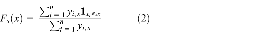
where
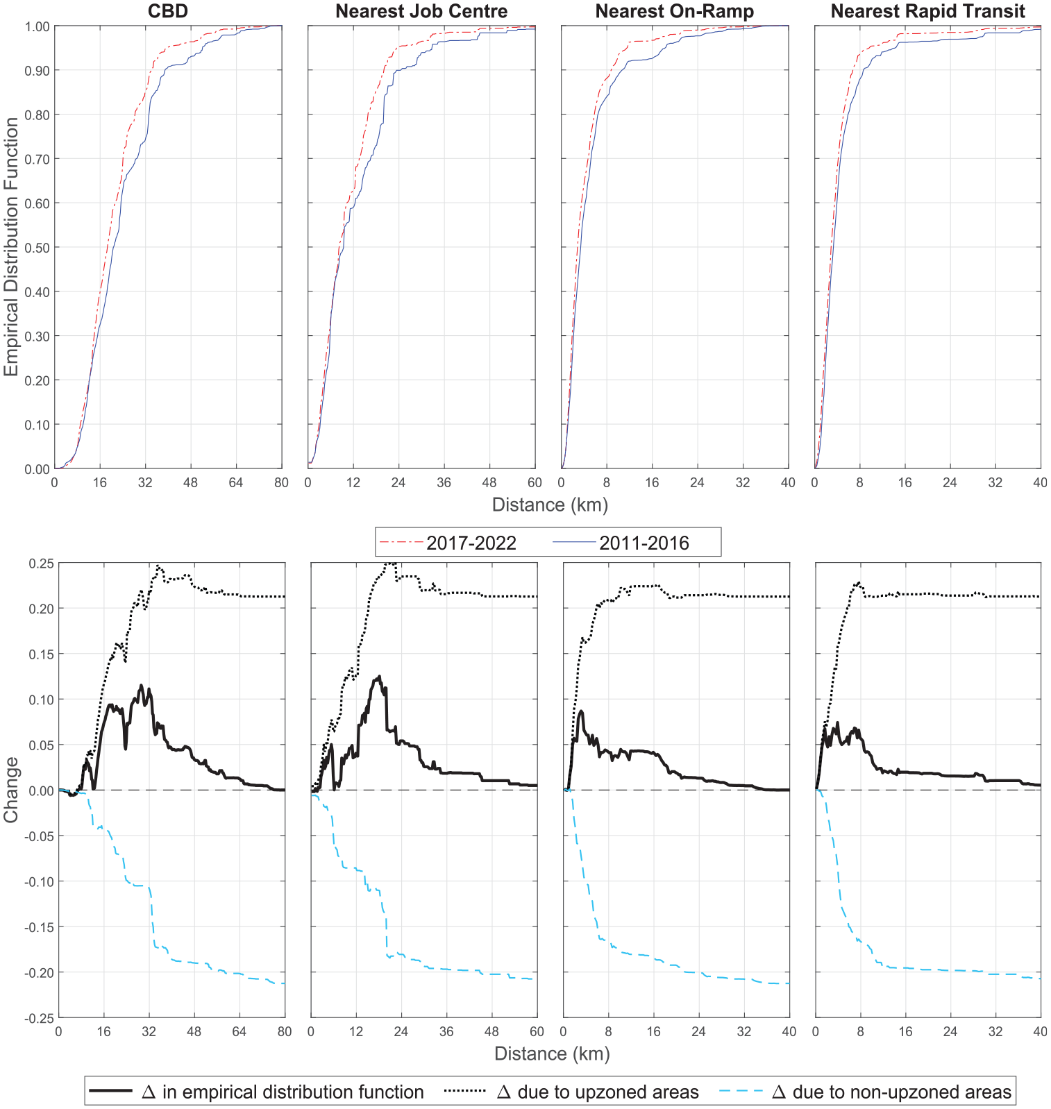
Spatial distribution of consents before and after upzoning.
The EDF for CBD has increased, showing that residential construction is moving closer to the CBD. For example, prior to the AUP, approximately 50% of consents were within 20 km of the CBD. After the AUP, 60% of consents were within this distance. Much of the contraction is occurring in the outer suburbs. The 25th percentile barely changes, from 13.2 km prior to the AUP, to 12.6 km after. Meanwhile the 50th and 75th percentiles shift from 19.9 to 17.9 km, and from 32.1 to 25.1 km, respectively. We see a similar pattern for nearest on-ramp, RT station and job centre: the spatial distribution of consents has contracted towards these locations.
The second row of Figure 5 depicts the difference in EDFs, namely
To examine whether the shift in the spatial distribution is driven by upzoning, we decompose the difference in EDFs into changes in upzoned and non-upzoned areas. Let
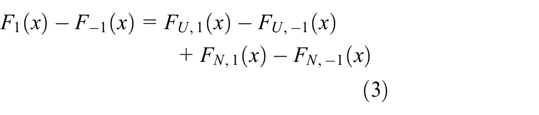
where
and
For each location, the contraction in the spatial distribution is being driven by changes in upzoned areas:
The near-uniform contraction in the distribution towards the CBD and job centres reverses an expansion prior to the AUP. Figure 11 in the Supplemental Material demonstrates that housing starts were expanding away from these areas prior to 2016, out to the 80th percentile of the EDFs.
Concluding remarks
Auckland’s zoning reform is notable for its scale and subsequent changes in housing development patterns. Subsequent to upzoning, housing starts have substantially increased; have contracted geographically towards the CBD, employment locations and transit network access points; and have become predominantly infill and attached housing.
Spatial decompositions reveal that these changes are due to substantial increases in housing starts in upzoned areas. This finding is consistent with economic models which also predict that upzoning causes an increase in housing supply. However, a limitation of empirical consistency is that it does not, as a general principle, in itself validate a model’s assumptions or causal mechanisms. While these models are standard in the field of economics, causal inference methods provide an alternative approach for assessing the effects of zoning changes on housing construction that are independent of a particular economic model (see Dong, 2024; Freemark, 2020; Greenaway-McGrevy, 2023; Maltman and Greenaway-McGrevy, forthcoming).
Auckland’s reform heralds lessons for potential reforms in other jurisdictions. Centralisation of planning decisions features prominently in the reform, through both the prior amalgamation into a single metropolitan jurisdiction and the central government’s willingness to pass laws to accelerate implementation. Fischel’s ‘homevoter hypothesis’ suggests that this centralisation was instrumental to implementation. Because development has concentrated costs and diffuse benefits, homeowners oppose local housing (Fischel, 2002). Regions with fragmented governance consequently have tighter restrictions (Fischel, 2008) and suboptimal development and sprawl. The corollary is that urban planning decisions should be centralised to the level at which the relevant costs and benefits of development are internalised, which is achieved by amalgamating fractured municipalities into a single authority.
However, while amalgamation is perhaps sufficient to enact successful reform, it need not be necessary. Allowing residents to collectively opt out, as occurred in Houston, may make zoning reform more politically acceptable. Direct monetary incentives from central or state government could overcome municipal opposition (Ehrlich et al., 2018). Finally, altering land use institutions to allow developers to bargain with neighbourhoods would enable affected residents to be compensated for bearing external development costs (Foster and Warren, 2022).
Notably, large-scale zoning reforms in North America, where metropolitan regions typically comprise multiple municipalities, have not relaxed as many restrictions as Auckland’s reform, and many appear to have had a comparatively limited impact on housing development to date. Minneapolis’ 2040 plan allows up to three dwellings per parcel, but does not relax restrictions on floorspace, and, as yet, has had no discernible effect on multifamily housing starts (Federal Reserve Bank of Minneapolis, n.d.). California’s HOME Act allows four dwellings per parcel, but has generated few permits, perhaps due to cities finding ways to subvert the policy (Garcia and Alameldin, 2023). Further research into contextual factors that moderate the effects of widespread upzoning will be an important next step to inform housing policy discourse. However, tentative conclusions from Auckland and North American experiences may be that (i) significant relaxations on floorspace restrictions in addition to reductions in minimum lot sizes enhance the efficacy of widespread upzoning, and (ii) ‘top-down’ impositions on unwilling municipalities may be less effective than ‘bottom-up’ initiatives. Maltman and Greenaway-McGrevy (forthcoming) provide another example of the latter from New Zealand: Lower Hutt.
Many social and environmental aspects of Auckland’s reform remain unexplored and deserve examination, including effects on spatial inequality, social mobility and environmental sustainability. By providing a framework for geospatially identifying the incidence and intensity of the reform, our article can assist in understanding these and other impacts.
Supplemental Material
sj-docx-1-usj-10.1177_00420980241311521 – Supplemental material for Can zoning reform change urban development patterns? Evidence from Auckland
Supplemental material, sj-docx-1-usj-10.1177_00420980241311521 for Can zoning reform change urban development patterns? Evidence from Auckland by Ryan Greenaway-McGrevy and James Allan Jones in Urban Studies
Footnotes
Appendix
Summary of land use regulations by residential zone under the Unitary Plan.
| Regulation | THA | MHU | MHS | SH | LL | RCS |
|---|---|---|---|---|---|---|
| Max. height | 16 m (5 – 7 storeys) | 11–12 m (3 storeys) | 8–9 m (2 storeys) | 8–9 m (2 storeys) | 8–9 m (2 storeys) | 8–9 m (2 storeys) |
| Height in relation to boundary | 3 m up+45° rp | 3 m up+45° rp | 2.5 m up+45° rp | 2.5 m up+45° rp | Does not apply | 2.5 m up |
| Setback (side and rear) | 0 m | 1 m | 1 m | 1 m | 6 m | 1 m |
| Setback (front) | 1.5 m | 2.5 m | 3 m | 3 m | 10 m | 5 m |
| Max. site coverage (%) | 50% | 45% | 40% | 35% | Lesser of 20% or 400 m2 | Lesser of 20% or 400 m2 |
| Max. impervious area (%) | 70% | 60% | 60% | 60% | Lesser of 35% or 1400 m2 | Lesser of 35% or 1400 m2 |
| Min. dwelling size (1 bedroom) | 45 m2 | 45 m2 | 45 m2 | n/a | n/a | n/a |
| Max. dwellings per site | Does not apply | 3 | 3 | 1 | 1 | 1 |
| Min. lot size (subdivision) | 1200 m2 | 300 m2 | 400 m2 | 600 m2 | 2500 m2 | 4000 m2 |
Notes: Restrictions are ‘as of right’ and can be exceeded through resource consent notification. Height in relation to boundary restrictions applies to side and rear boundaries. Less restrictive height in relation to boundary rules than those tabulated applies to side and rear boundaries within 20 m of site frontage. Number of storeys (in parentheses) is obtained from the stated purpose of the height restriction in the regulations. Planners have discretion in setting height in relation to boundary and setbacks in the large lot zone, with regulations requiring ‘development to be of a height and bulk and have sufficient setbacks and open space to maintain and be in keeping with the spacious landscape character of the area’. Maximum dwellings per site are permitted as of right. Minimum lot sizes do not apply to extant residential parcels. Impervious area is the area under the dwelling and structures such as concrete driveways that prevent rainwater absorption into the soil.
THA: Terraced Housing and Apartments; MHU: Mixed Housing Urban; MHS: Mixed Housing Suburban; SH: Single House; LL: Large Lot; RCS: Rural and Coastal Settlement; rp: recession plane.
Acknowledgements
We thank Auckland Council for providing the consents and code of compliance datasets, and information on the collection and collation of code of compliance certificate data. Jones thanks the Kelliher Trust for their support.
Declaration of conflicting interests
The author(s) declared no potential conflicts of interest with respect to the research, authorship, and/or publication of this article.
Funding
The author(s) disclosed receipt of the following financial support for the research, authorship, and/or publication of this article: This research was funded by the Royal Society of New Zealand under Marsden Fund Grant UOA2013.
Supplemental material
Supplemental material for this article is available online.
Notes
References
Supplementary Material
Please find the following supplemental material available below.
For Open Access articles published under a Creative Commons License, all supplemental material carries the same license as the article it is associated with.
For non-Open Access articles published, all supplemental material carries a non-exclusive license, and permission requests for re-use of supplemental material or any part of supplemental material shall be sent directly to the copyright owner as specified in the copyright notice associated with the article.