






Abstract
Geographic price differences confound comparisons of economic performance across cities by conflating nominal urban advantages with real differences in well-being. Existing tools only partially address this problem: the Bureau of Economic Analysis publishes a Regional Price Parity (RPP) Index that represents relative price levels in US cities and states, but it is available only annually since 2008 and with a publication lag, limiting its usefulness for historical or high-frequency analysis. To address this measurement gap, we use the Consumer Price Index (CPI) for 29 US cities to construct a CPI-based RPP, enabling consistent comparisons of urban economic performance over time at constant and comparable prices. We exploit standard price-parity properties using publicly available CPI data to estimate CPI-based RPPs at a higher frequency and over longer historical horizons. This results in a CPI-based RPP for any period with published CPI data, as far back as 1913 in some cities to the most recent observations. By separating nominal urban advantages from cost-of-living differences, the index allows researchers to reassess claims about urban well-being, affordability, and the real returns to agglomeration. We demonstrate the index by examining long-run regional price dynamics and comparing real per capita GDP and real per capita personal income across cities at constant and comparable prices.
Introduction
Comparing economic performance and well-being across cities can be misleading if the prices of goods and services differ significantly, distorting urban policy debates about affordability, density, land-use regulation, and metropolitan growth. For example, in 2023, per capita personal income was $69,893 in Honolulu, HI, and $63,789 in Tampa, FL, but the median rent of a three-bedroom home in Honolulu is 50% higher than in Tampa, 1 so it is not immediately clear which city offers higher living standards. Such comparisons sit at the core of urban debates over affordability, migration, inequality, and whether higher-income metropolitan areas deliver higher real returns to residents. Accounting for geographic price variation is therefore essential across urban and regional research, including labor markets, well-being, productivity, and place-based policy evaluation (Albouy, 2009; Gyourko and Tracy, 1991). Yet existing tools for adjusting urban data for price differences are limited, especially for high-frequency or long-run spatial comparisons. To help address this gap, we construct a consistent subnational Regional Price Parity (RPP) index for US cities using the US Consumer Price Index (CPI) and metropolitan area CPIs. Our CPI-based RPP can be applied (with the US CPI) to compare metropolitan economic outcomes at geographically comparable and constant prices. Our estimates do not require micro-level price data; instead, they re-level existing CPIs by adapting prior work from the Bureau of Economic Analysis (BEA) and extrapolate price levels over time based on differences between each city’s CPI and the US CPI for urban consumers, using standard price-parity-index principles.
Many questions in urban and regional research rely on geographic comparisons—including convergence, wages, productivity, inequality, and housing—yet most analyses use nominal data or national deflators that ignore spatial price variation. For example, Ganong and Shoag (2017) show that nominal income convergence across US states slowed after 1980, attributing this to spatial sorting driven by housing regulation in high-income regions. Without comprehensive price adjustment, however, it is unclear how much observed divergence reflects real differences in living standards. Similarly, Glaeser et al. (2009) note that measures of inequality are difficult to interpret when prices vary across locations and income groups. This limitation affects nearly all studies based on geographic comparisons (see, among many others, Florida and Mellander, 2016; Ganong and Shoag, 2017; Glaeser et al., 2008; Lee, 2011; Moretti, 2012).
The issue is equally acute for studies of economic mechanisms that hinge on location choices. Migration decisions reflect income opportunities (Greenwood, 1981; Kennan and Walker, 2011), amenities (Partridge, 2010; Rappaport, 2007), commodity prices (Bond-Smith et al., 2025), institutions (Parkins, 2010), welfare (Xie et al., 2021), and especially local cost-of-living differences, notably housing (Ganong and Shoag, 2017; Glaeser and Gyourko, 2018). When geographic price variation is ignored, nominal income differences cannot be interpreted as differences in real purchasing power or living standards.
Similar concerns arise across urban research, including studies of location wage premia (Farrokhi and Jinkins, 2019), agglomeration and productivity (Combes et al., 2011), housing affordability and real income distribution (Hsieh and Moretti, 2019), amenity valuation (Albouy, 2016), innovation and spillovers (Kemeny and Storper, 2015), and spatial equilibrium (Kemeny and Storper, 2012). The absence of consistent spatial price data limits inference, particularly in debates over migration and agglomeration, where the key question is whether higher nominal earnings in large metros translate into higher real living standards once housing and other urban costs—shaped by land use and urban form—are accounted for. By providing a long-run, CPI-weighted price parity series, our approach enables consistent estimation of the consumer-relevant cost offset to nominal agglomeration gains and sharper inference on the real returns to migration and urban growth.
While some sub-national cost-of-living indexes exist, most publicly available measures are ill-suited for urban analysis because they offer only cross-sectional snapshots, impose fixed consumption bundles across places, or require detailed microdata unavailable to most researchers (see, e.g. Council for Community and Economic Research, 2018; Curran et al., 2006). Within the US, the Bureau of Economic Analysis (BEA) has led efforts to measure geographic price differences, with experimental estimates in 2005 (Aten, 2006) and RPP reporting since 2014, covering the period back to 2008 (Aten, 2017; Bureau of Economic Analysis, 2023). Although the BEA RPP is the gold standard, its annual frequency, limited historical coverage, publication lag, and reliance on the Personal Consumption Expenditures (PCE) price index have constrained its use in urban studies, particularly for research on long-run urban change, housing affordability, and spatial adjustment. Because local CPIs are published more frequently and are more commonly used in urban and regional analysis, the absence of a long-run, high-frequency, CPI-consistent price parity index remains a key measurement gap, especially given evidence that regional price levels change at much higher frequencies (Nakamura and Steinsson, 2008).
Among the few studies that adjust for geographic price differences, most control only for housing costs and local inflation, yet their results underscore the need for more comprehensive indexes. For example, Moretti (2013) shows that nominal wage inequality is overstated because high-wage workers sort into high-cost cities. In particular, adjusting for local prices (largely housing, with limited coverage of other goods) substantially changes measured wage inequality across cities, highlighting both the importance of regional price deflation and the limits of housing-based proxies.
Prices vary across cities because local costs (especially labor and rent), transaction and transport costs, and imperfect arbitrage jointly shape local price levels (Engel and Rogers, 1996). City-scale forces further shift prices upward through dual-career sorting (Costa and Kahn, 2000) and downward through greater product variety (Handbury and Weinstein, 2015). These geographic price differences mean that the spending power of income and the real value of production depend on where they occur. As a result, nominally prosperous cities often deliver smaller real gains once higher prices are accounted for, while lower-income places benefit from lower costs, narrowing real differences in well-being. Applying RPPs therefore reduces measured regional inequality and substantially attenuates differences in living standards between skilled and unskilled workers when adjusted for local prices (Moretti, 2012, 2013). This motivates extending CPI-based adjustments beyond growth rates to levels of income and output, to assess urban well-being consistently across places and over time.
There are already several studies that measure geographic price differences within countries, though this literature primarily focuses on the construction of such measures, rather than their application. See Biggeri et al. (2017) for a survey of research on sub-national Purchasing Power Parity (PPP) indexes. More recently, the World Bank’s International Comparison Program has compiled a guide for a best practice method to compile within-country PPPs (Biggeri and Rao, 2021). Much of the research literature focuses on estimation methods. But without access to detailed price survey data, our focus is on the two key properties of geographic price parity indexes that we exploit to calculate indexes over a much longer period and at a much higher frequency, using metropolitan area CPIs and the US CPI. The OECD has explored estimating subnational purchasing power parities across countries using proxies such as housing prices and income levels (OECD, 2023). While such efforts offer valuable cross-sectional snapshots of spatial price variation, these methods are not designed to produce consistent time-series estimates. In particular, the reliance on housing-based regressions and cross-sectional data makes them unsuitable for constructing dynamic, multi-period RPPs.
The underlying theory of sub-national price-parity indexes comes from the concept of international Purchasing Power Parity (PPP) indexes. PPP indexes adjust for price differences to enable comparisons at comparable purchasing power (Taylor and Taylor, 2004), abstracting from distortions in exchange rates and local price levels. The same logic motivates sub-national price-parity measures: adjusting regional economic outcomes for differences in local purchasing power. In practice, while the BEA’s RPP applies this logic using the PCE basket, urban analysis often relies on the CPI to reflect out-of-pocket consumer costs, and its long-run, high-frequency metropolitan coverage makes it well suited for constructing CPI-based RPPs that support consistent analysis across cities, time, and historical periods.
To estimate our CPI-based RPP indexes, we build on BEA methods by estimating average CPI re-leveling factors for 2008–2022 to convert CPI movements into relative price levels rather than index-year changes, and apply absolute and relative price parity to extend these levels across time and frequency. This allows us to estimate CPI-based RPP indexes over several decades for 27 US cities, for more than a century in 19 cities, with two additional metros covered for shorter periods. These indexes support consistent comparisons of real wages, per capita income, GDP, housing affordability, and spatial inequality across cities and over time.
Estimating a CPI-based RPP
This section explains the calculations and data we use to estimate CPI-based RPPs for US cities and is designed to produce a price index suitable for applications in urban and regional research that require consistent adjustment for local cost-of-living differences. The method is based on the mathematical properties of price parity indexes using publicly available price indexes from the BEA and Bureau of Labor Statistics (BLS).
Mathematical properties of RPPs and price indexes
The idea of geographic price indexes is not new. Indeed, Purchasing Power Parity (PPP) was first coined by Cassel (1918) as the relevant exchange rate for countries to return to the gold standard after the war. Exchange rates deviate from the PPP rate because barriers hamper trade and currency exchange in one direction. Modern PPP rates are based on the same theory, but for a basket of consumption goods, not just gold, (Taylor and Taylor, 2004) such that

where

where
The BEA’s RPPs are constructed from detailed price and expenditure data, including CPI surveys and expenditure microdata from the American Community Survey. Because the BEA’s methodology relies on confidential microdata, it cannot be replicated or directly adapted by external researchers. However, after adjusting local CPI indexes to reflect relative price levels, the properties of absolute and relative price parity enable a relatively straightforward calculation of a CPI-based RPP. The BEA also exploits the properties of price parity indexes, as we do in this paper, to implicitly define a regional PCE price index, similar to local CPIs. Modifying equation (1) by replacing the local currency price of goods with a local price level index and the alternate country price of goods with a national price level index and rearranging enables the BEA to estimate regional price level indexes that are implicitly defined based on the mathematical property of absolute price parity. As a result, the Implicit Regional Price Deflator (IRPD) published by the BEA is calculated as:

where
Calculating the CPI-based RPP exploits the same properties. Rearranging this means that we require an index in which

where the subscript

allows us to extrapolate a CPI-based RPP for any period in which local price indexes are recorded.
We also use price index sub-indexes, which imply that the aggregate price index is a weighted average of the underlying sub-indexes. Specifically, we assume that
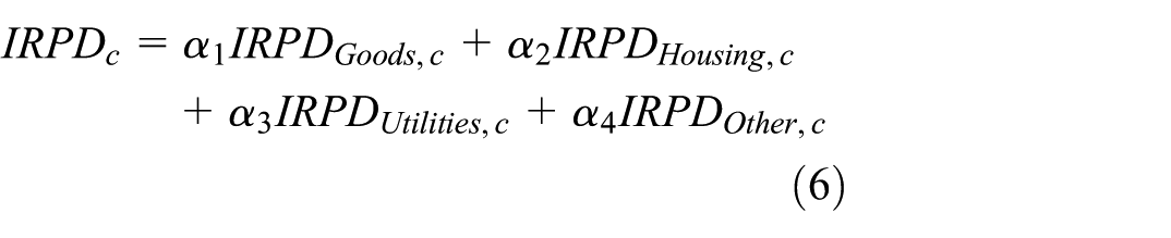
where

where
However, the BEA does not publish IRPDs for sub-indexes, but it does publish RPPs for sub-indexes. Therefore, the IRPD sub-indexes are calculated from the RPP sub-indexes in exactly the same way as the IRPDs are calculated from RPPs as specified in equation (3). Specifically,

where the subscript label refers to each of the sub-indexes: Goods, Services:Housing, Services:Utilities, and Services:Other. We use all of these mathematical properties to estimate CPI-based RPPs.
Initial calculations
We first make a few intermediate calculations using the BEA’s RPP data. We calculate IRPD sub-indexes from the BEA’s RPP and its RPP sub-indexes (See equation (8)). We also calculate an implied IRPD for the metropolitan portion of the US. This is necessary for our method to adjust the national CPI to price levels because the US CPI represents prices for all urban consumers. So, we assume that the national PCE, indexed to 2017, is a population-weighted average of metropolitan and non-metropolitan portion IRPDs. 2 Rearranging this weighted average, the implied IRPD for metropolitan areas is
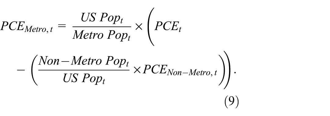
Estimating a CPI price level
The CPIs published by the BLS are indexed to an average of 100 in 1984–1986. So, differences in the level of the CPI in different cities only tell us about relative price changes since that index period and do not include the extent to which price differences already existed. Therefore, we need to re-level the CPIs using a CPI price re-leveling factor that we estimate from the BEA’s IRPDs and IRPD sub-indexes. We use a sequential least squares programming (SLSQP) algorithm of CPI sub-indexes (comparable to the IRPD sub-indexes) to estimate relevant weights of these sub-indexes in the CPI for each urban area and the US overall over 2008–2022—the period with IRPD data from the BEA at the time of writing. We apply these weights to the IRPD sub-indexes to estimate average CPI price levels over this period.
The comparable CPI sub-indexes are Commodities (eq. to IRPD Goods); Shelter (eq. to IRPD Services: Housing), and Services less rent of shelter (eq. to the combination of IRPD Services: Utilities and IRPD Services: Other). Since the third CPI sub-index is a one-to-two match with the IRPD sub-indexes, we first estimate a weighted average of IRPD Services: Utilities and IRPD Services: Other:
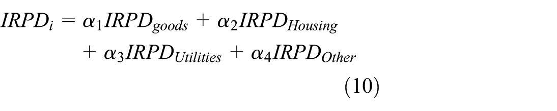
where
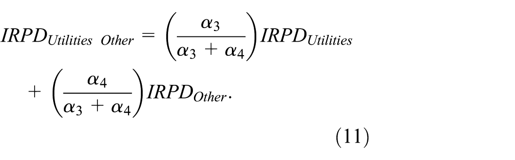
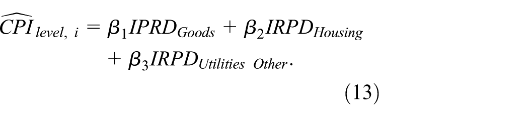
Similarly, we assume CPIs in each city are a weighted average of local CPI sub-indexes, and we estimate a regression to find the weights for each sub-index,

where
We use these weights with the IRPD sub-indexes to estimate local CPIs in relative price levels.
The ratio of the average estimated local CPI in levels to the average local CPI,

Re-leveling is equivalent to re-indexing but targeting the estimated average levels rather than a particular year. So, the final estimates of
Calculating the CPI-based RPP
After re-leveling local CPIs and the US CPI for all urban consumers, we calculate a CPI-based RPP index for the 29 US metropolitan areas with CPIs published by the BLS. This means that CPI-based RPP rates are available for any period and frequency where CPI data is published. It is calculated using the mathematical property of absolute price parity shown in equation (1):

This CPI-based RPP also achieves the mathematical property of relative price parity.
Data
The data requirements for our approach are not intensive. Calculating the re-leveling factors requires annual CPIs for each Metropolitan Statistical Area (MSA) and the US, as well as CPI sub-indexes for Goods, Shelter, and Services less rent of shelter between 2008 and 2022, to match the IRPDs published by the BEA or calculated in our initial calculations. The CPI-based RPPs are calculated for any period in which CPI-data is published.
The BLS publishes monthly CPI observations for the US and monthly, two-monthly, or sometimes three-monthly CPIs for individual MSAs. In addition, the BLS publishes annual and semi-annual observations. Observations are less frequent during historical periods, and occasionally, some observations are missing. For our estimates of weights, we use the annual figures between 2008 and 2022 to match the frequency and period covered by the IRPDs published by the BEA.
In six cities (Pittsburgh, PA; Cleveland-Akron, OH; Milwaukee-Racine, WI; Cincinnati-Hamilton, OH-KY-IN; Kansas City, MO-KS; and Portland-Salem, OR-WA) the BLS stopped publishing CPIs in 2018, with the last annual observation in 2017, so the regressions for these cities use data for 2008–2017. Similarly, the CPI in Riverside-San Bernardino-Ontario, CA, is only available for the period since 2018, so for this city the regressions only used data for 2017–2022. With fewer data points, this creates a risk that the estimates of the CPI re-leveling factors are less accurate in these cities, but the weights estimated are very similar for all cities, so we are not concerned about this risk, though we are cautious of using the estimate for Riverside. For all other cities, we use the full period from 2008 to 2022.
In two cities (Washington-Arlington-Alexandria, DC-VA-MD-WV, and Baltimore-Columbia-Towson, MD), seven of the 15 annual CPIs were not reported, but two-monthly observations were reported. So, we calculate the annual observation as an average of monthly observations with straight-line extrapolation of months in-between the two-month-to-two-month observations which are comparable to the observed annual CPI observations in cities where these are reported.
Outputs
Our CPI-based RPP estimates are available for any period in which CPI data are published. 3 For recent periods, this is usually a two-month-to-two-month frequency for each MSA, but some MSAs such as New York-Newark-Jersey City, NY-NJ-PA have monthly data since September 1940. For any missing observation, we also publish monthly RPPs based on extrapolations between CPI observations. Alongside monthly data, we report semi-annual and annual observations of RPPs based on the BLS reported annual and semi-annual CPIs.
There are historical periods with differing frequencies, including some years with three-monthly observations or as low as just one month in the year observed, especially in more historic time periods over a century ago. Different cities are also often on different two-month-to-two-month reporting cycles, making the estimated CPI-based RPPs in different places inconsistent in the time periods reported. And lastly, there are occasionally observations missing.
Given the missing observations, there are two sets of results. Firstly, there is a set of CPI-based RPPs for the periods when the BLS has reported CPIs. But to make the data more useful, we straight line extrapolate missing monthly CPI observations or calculate any missing semi-annual and annual observations from period averages to fill in any missing data periods. We then also calculate the CPI-based RPPs from this complete series. This allows researchers to use the resulting CPI-based RPPs for any frequency and time period within the time ranges for which CPI data are available.
Comparing our results to the BEA’s RPPs helps to assess the plausibility of our estimates and any divergences (see Figure 1). The two RPP measures track each other closely in most metros, confirming that they share the same broad spatial and temporal signals. Where they differ, the CPI-based series is systematically higher in metros with higher housing costs (e.g. San Francisco, Los Angeles, San Diego, Seattle, Denver, Miami, and Urban Hawaii) and slightly lower in Midwest metros with cheaper housing. Moreover, the gap is time-varying: it tends to widen during housing booms—most visibly after the mid-2010s and again post-2020—consistent with the greater weight for housing costs in the CPI, making it more sensitive to higher rents and house prices. Despite these level differences, the ranking of high- and low-cost cities is generally stable across measures. The alignment between our CPI-based RPPs and the BEA series provides a strong plausibility check: both measures deliver very similar levels and time paths across metros and any gaps are concentrated in places where shelter costs are known to be especially high, which is exactly where a CPI-weighted basket can be expected to diverge from a PCE-weighted one.
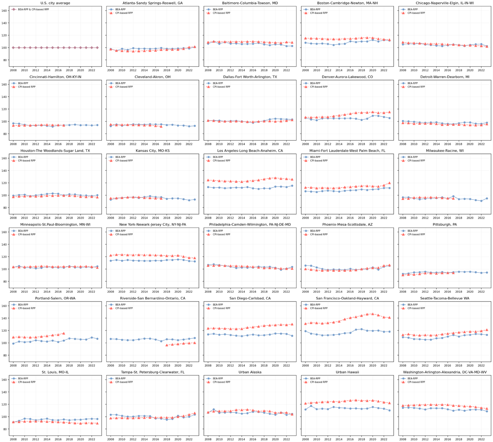
BEA versus CPI-based RPPs.
The CPI-based RPPs offer three distinct advantages: (1) the frequency of observations (typically bimonthly, and monthly in some metro areas); (2) the availability of recent data (allowing construction of a plausible current RPP); and (3) historical coverage (with series in some MSAs extending back more than a century). The advantage of the BEA indexes is their geographic coverage, but they are only published annually, with a one-year delay, and only back to 2008. By enabling price-level adjustment at high frequency and over long historical horizons, our CPI-based RPP expands the scope of empirical urban analysis beyond what has previously been feasible with existing price indexes.
CPI-based RPP price trends
In this section, we explore the resulting CPI-based RPP levels and trends in the 29 cities.
The geography of relative prices
Figure 2 shows the CPI-based RPP indexes in 1918, 1965, and 2023 for comparisons geographically and between time periods. We use these dates as the start and ends of our data range for most cities, and an intermediate date when several more cities were added.
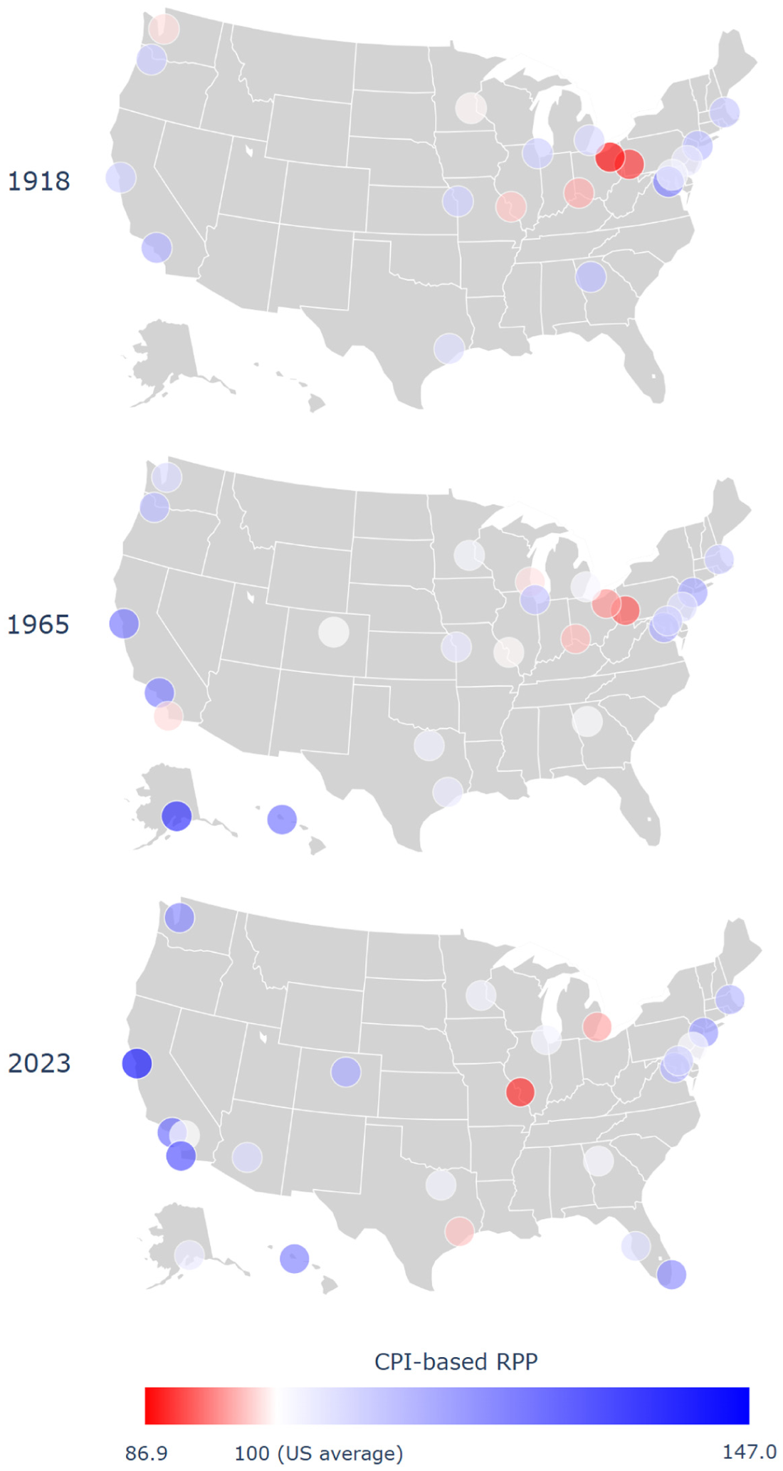
US Map of CPI-based RPPs (1918, 1965 and 2023).
Notably, price trends are spatially uneven. Inland cities are usually relatively lower cost compared to coastal cities and saw declining relative price levels between time periods. Midwestern cities like Kansas City and Pittsburgh typically have lower-than-average. Cities around the Rust Belt, like Detroit and Chicago, saw relative price declines. Cities on the East Coast tended to be consistently more expensive than average, while cities on the West Coast tended to experience relative price increases. But these geographic patterns are not uniform either. Anchorage has become considerably less expensive, while Denver has become considerably more expensive.
Relative price levels
Figure 3 shows our CPI-based RPPs for each MSA over time, emphasizing the five top and bottom MSAs based on the average values of their CPI-based RPPs.
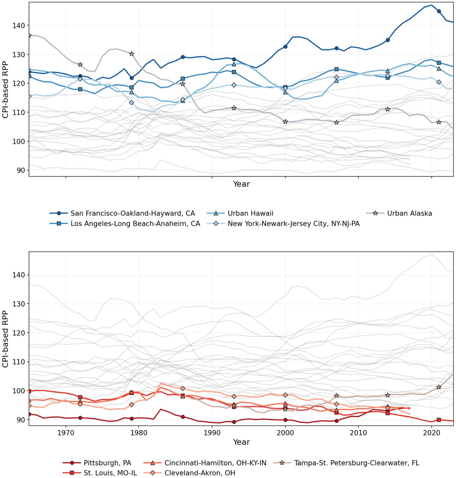
Top and bottom five MSAs by average CPI-based RPP, 1965–2023.
In the first chart, the city with the highest average price level is shown in a darker shade of blue, while lighter shades indicate lower price levels. The CPI-based RPP for San Francisco-Oakland-Hayward, CA, has increased gradually and continuously but was already elevated in 1920. It reached a brief peak in 2000 and its highest peak at 150 in 2020. That is, for a CPI basket of goods, San Francisco had prices about 50% higher than the average in 2020. Los Angeles-Long Beach-Anaheim, CA, and Washington-Arlington-Alexandria, DC-VA-MD-WV, also had increases in prices between 1915 and 2023, though at a much slower growth rate and often with long periods of declines too. Urban Honolulu, HI, and New York-Newark-Jersey City, NY-NJ-PA, on the other hand, have maintained relatively similar, but still elevated, price levels over time.
In the second chart, the city with the lowest average CPI-based RPP is shown in the darkest shade of red, while others are lighter shades based on their levels. Cities in the bottom five have generally maintained their relatively lower price levels over time, mostly ranging between 90 and 100 throughout the entire period. There was a slight upward shock in price levels in the 1980s in a few of these cities, but relative prices returned to their long-run average by 1990. More recently, Tampa-St. Petersburg-Clearwater, FL has shown a rapid increase in its relative price level since 2020, although arguably since around 2000. A number of factors could explain this spike.
The locations and geography of these cities generally implies a few possible explanations. Larger cities tend to have higher prices that reflect the real estate market’s higher prices, scarcity of supply, and the value of proximity to large city centers, as well as the greater willingness and ability to pay when residents earn higher incomes due to agglomeration economies. Cities in isolated places, like Hawaii and Alaska, which were not in the top five, also have higher prices, due to higher transportation and transaction costs. Prices diminished over time in Urban Alaska, but the popularity of Hawaii as a tourism destination has meant that Honolulu did not experience the same relative price level declines as Anchorage. Inland cities perhaps have greater land availability, reducing the cost of housing. Finally, growth in the US has been concentrated in a handful of coastal, superstar cities, and prices often reflect income growth.
Relative price changes
While the above discussion compared cities by their relative price levels, referring to the magnitudes of the CPI-based RPPs, here we specifically focus on relative price changes over time, focusing on 1965 onward as this period captures more cities. We categorize MSAs into five groups: cities where relative prices increased by at least 5%, cities where relative prices decreased by at least 5%, and cities with prices that maintain a stable level, within plus or minus 5% of the initial value, but classified by high, moderate, and low prices relative to all urban consumers. To be clear, all cities faced aggregate inflation of more than 5% over this long period, but the CPI-based RPP measures relative prices compared to the average for the US overall, and we categorize them by the relative increase or decrease in their CPI-based RPP value. We categorize cities with three levels of relatively stable prices within 5% and the 5% change threshold because this generates five groups that are about equal in size, and we examine percentage change in the CPI-based RPP value because it allows for a fair comparison between cities with otherwise differing relative price levels.
Figure 4 summarizes the categories by plotting the CPI-based RPP in 1965 (or initial year) compared to 2023 (or final year) with lines depicting the region in which prices changed by more or less than 5%. Notably, relative price levels usually persist, with most MSAs within the 5% change band. For example, Urban Hawaii has always been expensive, with only a slightly lower relative price level in 2023 compared to 1965. Similarly, Pittsburgh was always a relatively low-cost city and, in 2017, was only slightly above its relative price level in 1965.
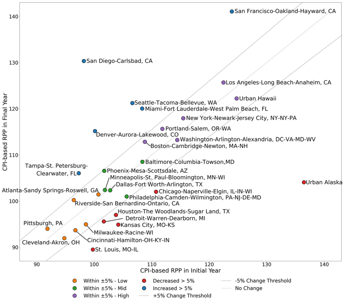
CPI-based RPP in 1965 or initial year versus 2023 or final year by Category.
Cities with accumulated CPI-based RPP increases of at least 5%, are primarily tech centers in California and Washington and cities with a desirable climate in Florida, both factors that could be driving demand for real estate and factors of production, increasing prices. Conversely, MSAs where the CPI-based RPPs declined by at least 5% appear related to industrial and population decline, in the case of Detroit and Chicago, an abundant supply of real estate and housing, such as Kansas City and Houston. The major outlier here is Urban Alaska, which could be due to a large decline in the cost of isolation and geography on prices, although counteracting forces may have prevented this decline in Urban Hawaii.
There are a number of different explanations that might explain why high-priced cities sustained high, stable relative prices (which remain within 5% of their initial value, but are consistently at a higher level than the average for all urban consumers at 100). As noted above, Urban Hawaii and Urban Alaska had high prices in 1965—likely related to their geographic isolation—but prices remain elevated in Hawaii, perhaps partly due to its desirable amenities, a large tourism industry, and a restricted housing market (Tyndall et al., 2023). That said, prices fluctuated considerably, with declines by almost 10% relative to the initial price level in the 1970s and early ’80s and again in the 1990s after a peak in the early ’90s. Los Angeles and New York appear in this list mostly due to population size. Boston-Cambridge-Newton, MA-NH probably maintains high prices both through city size and a strong local economy. Washington-Arlington-Alexandria, DC-VA-MD-WV, hosts the federal government and a relatively higher-skilled workforce with higher incomes. In all of these cities, restrictive land-use policies are also likely to play a role.
Moderately priced MSAs with stable relative prices (within 5% of their initial value, but at a moderate price level) include larger regional inland cities. These cities can benefit from an abundant land supply since they are not geographically constrained by a coastline, and are often also less geographically constrained by mountains. Anecdotally, Baltimore is relatively lower cost because of industrial decline, but it did not fall into the declining category, likely due to its proximity to the DC metro area. Similarly, low-priced MSAs with stable prices (within 5% of their initial value, but at a relatively low price level) are also inland, with abundant land supply keeping prices for real estate low. Industrial decline will also likely play a role in persistently low price levels. While Riverside, CA, is in this group, it only has data since 2018 and has rising prices, so it would likely be part of the rising price group if more time periods were available.
Applying the CPI-based RPP to economic performance measures
The ultimate purpose of the CPI-based RPPs are to fairly adjust economic outcomes to reflect well-being afforded by economic activity in different cities and to consider the extent that observed urban advantages actually reflect productivity or higher costs. We apply the CPI-based RPPs to adjust two key measures of regional economic performance: GDP per capita and per capita personal income. These CPI-based RPPs could also be applied to any other monetary measure of economic performance. By adjusting for regional price differences, these indicators reflect the actual local value of economic activity and income to give a more accurate reflection of the well-being achieved in different cities.
GDP per capita
We compare real GDP per capita for cities from 2001 to 2023 in constant 2023 dollars, firstly adjusted for inflation only and then also adjusted by CPI-based RPPs. We examine this period as GDP data is available by MSA back to 2001.
Per capita GDP is adjusted downward by the CPI-based RPP in high-cost cities such as Honolulu, New York, and San Francisco. At the other end of the scale, per capita GDP is adjusted upward by the CPI-based RPP in relatively low-cost cities such as St. Louis, Detroit, and Atlanta. So, this adjustment tends to bring thriving and lagging regions closer together in terms of geographic-price-adjusted economic activity.
In most cases cities generally maintain their relative position because price levels are correlated with per capita GDP, but the distribution of outcomes across cities is much narrower. From an urban perspective, this suggests that much of the apparent economic dominance of high-cost metropolitan areas partly reflects higher prices. The exception to this general ranking rule is Urban Hawaii, which drops from the middle of the range to near the bottom, reflecting its consistently higher price levels despite modest incomes. So, when real per capita GDP is not adjusted for geographic price differences, it appears to mask a persistent lag in economic outcomes in Hawaii.
In addition to these level effects, adjusting per capita GDP for the CPI-based RPP also affects growth rates if cities have relatively higher or lower inflation rates than the US overall. Cities with rising prices, such as San Francisco, experienced relatively lower GDP growth than shown by real per capita GDP unadjusted for geographic price differences. On the other hand, cities that experienced relatively lower inflation than the US overall, such as Houston-The Woodlands-Sugar Land, TX, show higher per capita GDP growth after adjusting for geographic price differences.
Figure 5 shows how adjusting for CPI-based RPP affects real per capita GDP growth. The bars show real compound annual growth rates of per capita GDP and the red dot shows how these estimates change when real per capita GDP is adjusted for geographic price differences with our CPI-based RPPs.
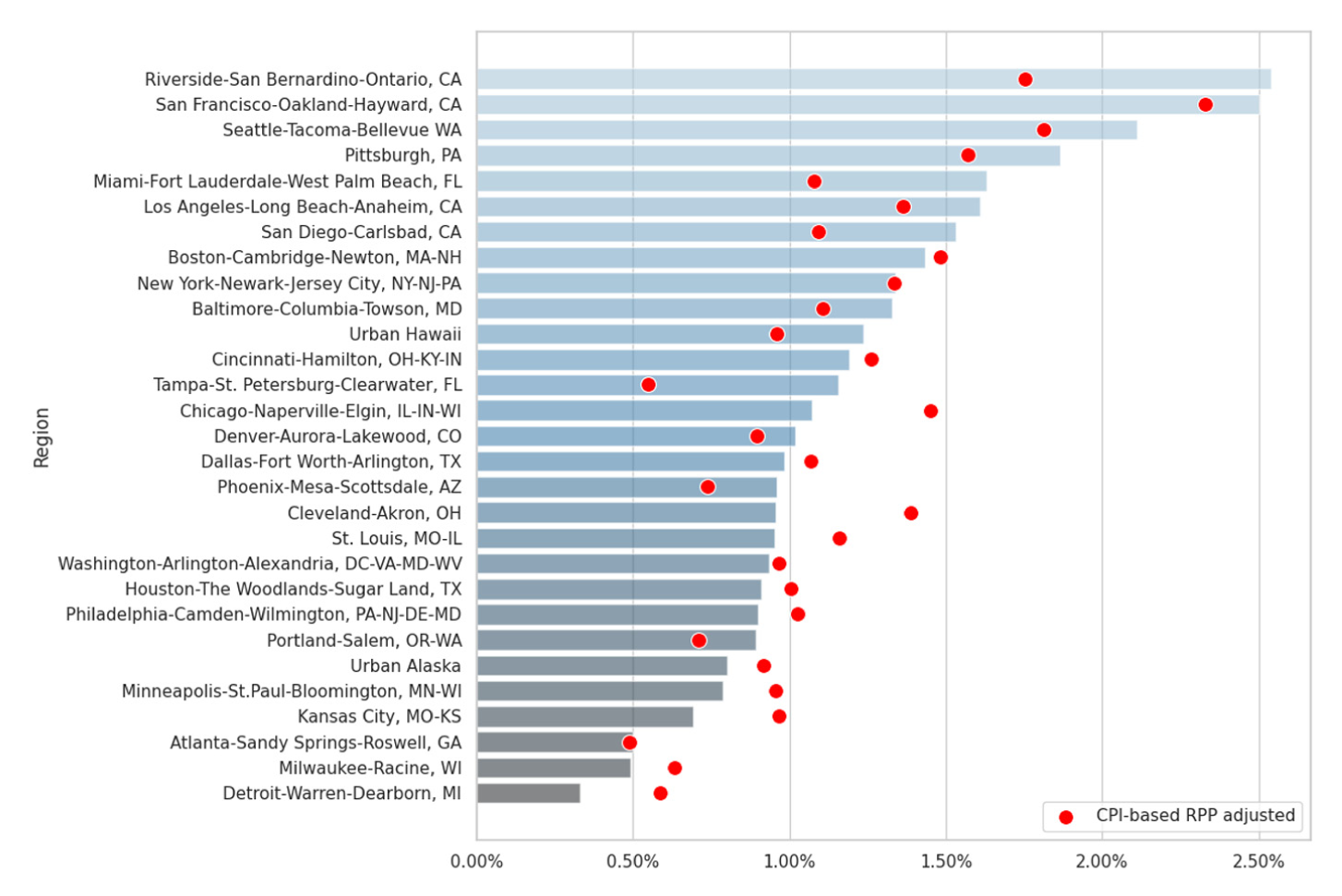
Real GDP per capita Average Compound Annual Growth Rate 2001–2023.
While Riverside-San Bernardino-Ontario shows a substantial annual growth rate (over the shorter period of CPI data), much of this growth is lost to relatively higher inflation. The two cities in Florida show significant adjustment downward in growth rates due to relatively higher inflation with Miami’s CPI-based RPP increasing from 106 in 2000 to 120 in 2023, and Tampa’s CPI-based RPP increasing from 92 in 2000 to 106 in 2023. Surprisingly, San Francisco’s growth rate diminishes only slightly, reflecting that its price level was already elevated in 2000 and remained relatively flat for the next decade.
The charts highlight the importance of adjusting (or interpreting) economic performance measures for relative price differences in order to accurately understand urban well-being. Some places that otherwise appear to lag behind the leading cities according to unadjusted real GDP per capita growth rates, such as Chicago and Cleveland, are actually doing better than average according to CPI-based RPP adjusted Real GDP per capita.
Income
We also examine per capita personal incomes from 1969 to 2023 in constant 2023 dollars, firstly adjusted only for inflation and then also adjusted for our CPI-based RPPs.
Major global cities, such as New York and San Francisco, still show high incomes, but the magnitude has been reduced by around $10–30k in 2023. Similarly, real incomes in low-cost cities such as Pittsburgh and Kansas City increase after the CPI-based RPP adjustment, reflecting the well-being afforded by a lower cost of living. These adjustments are especially relevant for urban research on affordability and displacement, where nominal income growth may coincide with stagnant or declining real purchasing power for residents.
Figure 6 shows how adjusting for CPI-based RPPs affects the average annual growth rate of real per capita personal incomes. The bars show real income growth, while the blue squares show real income growth, also adjusted for our CPI-based RPPs.
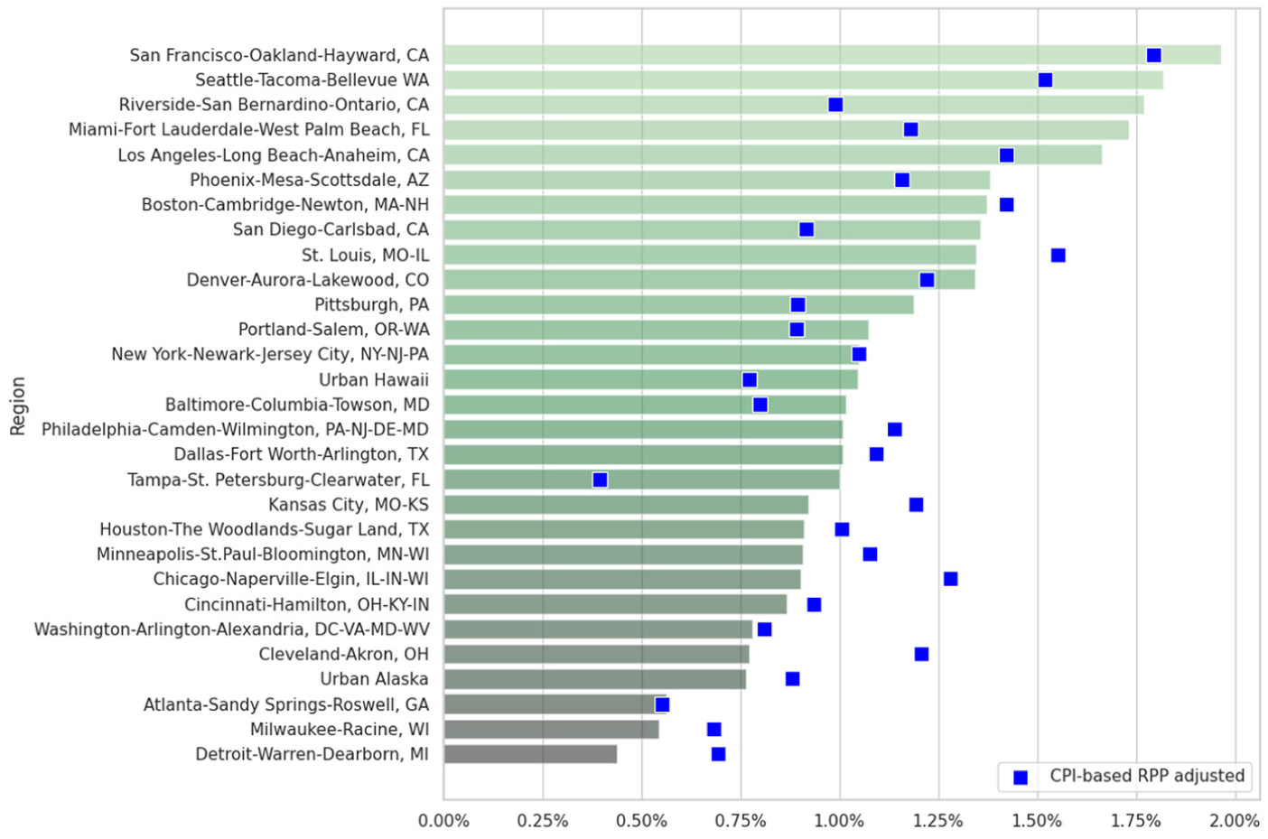
Real per capita personal income average compound annual growth rate 1969–2023.
Income growth in San Francisco remains relatively strong after adjusting for relative price levels with only a slight downward shift, reflecting that San Francisco already had elevated prices in 1969 and only slightly higher rates of inflation in most years than the US overall. But again, in Riverside-San Bernardino-Ontario, CA, recent per capita income growth is diminished significantly by the increase in prices, albeit over the much shorter period that CPI data is available. On the other hand, St. Louis, MO-IL, now experiences the second-highest real income growth rate among these cities, reflecting the gains in well-being due to relative price level declines. For urban research, these growth-rate adjustments matter because they show that nominally fast-growing metros can deliver much smaller gains in resident welfare once relatively faster rising urban costs—especially shelter—are accounted for, altering conclusions about the real returns to living in high-growth cities. This dynamic is evident in classic high-income metros such as San Francisco–Oakland–Hayward, but it can also arise in peripheral metros such as Riverside–San Bernardino–Ontario, where measured growth may partly reflect housing-price spillovers and decentralization from the Los Angeles region rather than stand-alone local productivity gains.
Concluding remarks
This project offers credible, CPI-based RPPs that describe relative price levels of the CPI baskets of goods in the 29 cities where CPIs are published by the BLS, as far back as 1913 and through to the most recently published CPI observations. The CPI-based RPPs are consistent with the mathematical properties of both absolute and relative price parity, which we use to calculate them. Importantly, the CPI-based RPPs can be calculated with any CPI observations, whenever they are published by the BLS, which is usually at a two-month-to-two-month frequency for most cities and has been published for several decades. As a result, the CPI-based RPP offers a suitable price-adjustment index to allow fair comparisons of regional economic data at price parity, high frequency, and over a long historical period through to the most recent observations. Combined with the US CPI, such comparisons can also be made at constant and comparable prices.
Our intention is that the CPI-based RPP provides a long-run, consumer-relevant price adjustment that supports more credible comparisons of urban well-being across space and time. This allows existing conclusions about urban economic performance to be reconsidered in light of geographic price differences. More broadly, the series provides a practical tool for reassessing the magnitude and evolution of real urban wage premia and the welfare gains from agglomerated labor markets. In doing so, policymakers can respond in ways that recognize the effects of both economic growth and urban planning on well-being by properly accounting for the cost of living. In particular, our results and others show how the thriving superstar cities did not benefit as much from growth as nominal figures imply (Glaeser and Gyourko, 2018; Gyourko et al., 2013; Hsieh and Moretti, 2019). This distinction is especially relevant in cities facing affordability constraints, where nominal income growth may mask declining real purchasing power. Adjusting for geographic price differences brings thriving and lagging places much closer together in terms of economic outcomes. Before this project, adjusting for local inflation allowed policy-makers to consider local price changes, but not price levels, and regional comparisons risked being misleading.
Adjusting for price levels may be particularly important for federal place-based policies, where the allocation of funding is partly driven by relative levels of income or GDP. For example, the Code of Federal Regulations (CFR)—used by the Economic Development Administration for particular grants—defines regions that are economically distressed. One requirement is for a region to have “Per capita income that is, for the most recent period for which data are available, 80 percent or less of the national average per capita income” (13 CFR 301.3(a)(1)). Adjusting for price levels would offer a more accurate reflection of economic distress by accounting for the local out-of-pocket purchasing power of per capita income.
For urban research, the index enables sharper distinctions between productive agglomeration benefits and housing-driven cost escalation. In much of the empirical literature, high nominal wages, incomes, and output in large metropolitan areas are interpreted as evidence of superior economic performance or stronger agglomeration forces, even though these same places often face substantially higher prices—most notably for shelter. A consistent geographic price deflator makes it possible to better distinguish these channels and to ask whether observed metropolitan “success” reflects higher real purchasing power or primarily higher costs that absorb much of the nominal advantage. This reframing is central to comparative work on spatial inequality and convergence, and it is especially relevant in settings where housing supply constraints, land-use regulation, and local amenities generate persistent differences in price levels across cities. The CPI-based RPP supports credible urban welfare assessments across space and time by supporting high-frequency real comparisons over longer historical horizons.
For urban planners and local governments, the indexes also provide a consistent framework for evaluating urban development strategies, since nominally higher incomes can coexist with stagnant or declining real living standards when rents and land values rise faster than earnings. In this way, the CPI-based RPP series can inform evaluations of local planning and housing institutions to assess whether they are accommodating real income advantages. In this sense, the CPI-based RPP offers a practical tool for interpreting the distributional and affordability consequences of urban policy and housing supply constraints.
More broadly, the series facilitates empirical work that links urban form, housing markets, and economic outcomes to resident welfare rather than nominal performance alone. In particular, it supports research that treats the cost of living—especially shelter—as an endogenous component of urban change rather than being absorbed implicitly by fixed effects. With a consistent geographic price adjustment, researchers can more directly evaluate how land-use regimes, housing supply elasticities, and neighborhood change shape the extent to which nominal income gains translate into real improvements in living standards. In this way, the CPI-based RPP strengthens empirical work on affordability, displacement pressures, and the welfare consequences of metropolitan expansion, densification, and decentralization.
Lastly, we aim to promote the development of alternative RPP indexes. Such research could help to improve the estimates of our re-leveling factors, increasing confidence in a CPI-based RPP. Academic debate would also help to refine other publicly reported indexes that can be misleading. Or research could offer new RPPs, such as ones representing the basket of goods produced locally, to help understand real productivity in different places at comparable prices: a regional RPP equivalent of the national GDP deflator. Of course, it is even possible that the BLS could consider publishing its own CPI-based RPP (and implied CPI-based re-leveling factors that translate the CPI to relative price levels) using its extensive CPI survey data. In any case, we appreciate the indexes published by both the BEA and BLS, and look forward to future developments.
Supplemental Material
sj-pdf-1-usj-10.1177_00420980261457721 – Supplemental material for Estimating a CPI-based regional price parity index for US cities
Supplemental material, sj-pdf-1-usj-10.1177_00420980261457721 for Estimating a CPI-based regional price parity index for US cities by Steven Bond-Smith and Younghan Lee in Urban Studies
Footnotes
Acknowledgements
We thank the Bureau of Economic Analysis for their work developing and producing regional price parity data and publishing a detailed methodology, which we use extensively in this article. We are also grateful to the Bureau of Labor Statistics for publishing Metropolitan Area CPI data, often for over a century, which allows the price parity indexes produced in this article to cover an extended period. For helpful comments and suggestions, we are grateful for comments from participants at the North American Regional Science Council Annual Meeting.

Funding
The authors disclosed receipt of the following financial support for the research, authorship, and/or publication of this article: This research was supported by a Research Support Award from the College of Social Sciences at the University of Hawai‘i at Mānoa.
Declaration of conflicting interests
The authors declared no potential conflicts of interest with respect to the research, authorship, and/or publication of this article.
Notes
References
Supplementary Material
Please find the following supplemental material available below.
For Open Access articles published under a Creative Commons License, all supplemental material carries the same license as the article it is associated with.
For non-Open Access articles published, all supplemental material carries a non-exclusive license, and permission requests for re-use of supplemental material or any part of supplemental material shall be sent directly to the copyright owner as specified in the copyright notice associated with the article.
