






Abstract
The current study examined the association between playing high school football and involvement in violent behaviors in sibling pairs drawn from the National Longitudinal Study of Adolescent Health (Add Health). The analysis revealed that youth who played high school football self-reported more violence than those youth who did not play football. Quantitative genetic analyses revealed that 85% of the variance in football participation was the result of genetic factors and 62% of the variance in violent behavior was due to genetic factors. Additional analyses indicated that 54% of the covariance between football participation and violence was due to genetics and 46% was the result of nonshared environmental influences. However, even after controlling for genetic influences, participation in football appeared to increase violent behavior.
During almost every professional athletic season, there are a series of high-profile athletes who engage in acts of serious physical criminal violence (Benedict, 2004; Benedict & Yaeger, 1998; Otto, 2009). This is particularly true for two of the most popular American professional sporting events of football and basketball, wherein media reports and TV channels devoted to covering issues related to sports routinely air documentaries and provide coverage to the latest criminal scandals plaguing the professional sporting industry. During the past couple of decades, moreover, there have been a number of published reports indicating that the prevalence and incidence of criminal acts are disproportionately high among professional football and basketball players, as well as for athletes from other less popular sports, such as boxing and hockey (Otto, 2009; but see Blumstein & Benedict, 1999). Although gaining a reliable and accurate estimate of the extent of criminal involvement among professional athletes is exceedingly difficult, the most consistent estimates suggest that approximately 32% of all professional football players and about 40% of all professional basketball players have been arrested for a crime (Benedict, 2004; Benedict & Yaeger, 1998). These numbers paint an alarming picture of the relatively widespread use of violence among professional athletes, a particularly problematic issue given that professional athletes are frequently viewed as heroes and role models among youth.
The potential association between violence and athletic participation is not confined solely to professional athletes, as there is also empirical evidence that participation in certain sports is associated with increased use of violence and misconduct at the collegiate level (Crosset, Benedict, & McDonald, 1995; Crosset, Ptacek, McDonald, & Benedict, 1996). Rule infractions, drug use, and even physical and sexual assaults have been found to be much more common among student-athletes than among college students who do not participate in an NCAA sport (Crosset et al., 1996; Cullen, Latessa, & Byrne, 1990). The link between violence/misconduct and athletic participation also appears to trickle down to high school sports. Indeed, some of the most methodologically sound studies examining the potential criminogenic effects of sports participation have analyzed samples consisting of high school students. While there is variability in findings across studies, a relatively consistent finding is that male athletes who participate in certain types of contact sports, especially football, self-report more involvement in aggression and delinquency than youth who participate in sports other than football or who do not participate in any sport (e.g., Kreager, 2007).
If these studies are correct, and there is a link between participating in football and the use of violence, then the next logical step is to begin to uncover the mechanisms that are responsible for producing this association. Although a number of explanations have been advanced, and some of these explanations have been tested using quantitative methodologies, there is not a single study to our knowledge that has ever examined the potential role of genetic factors. The aim of the current study is to address this gap in the literature by using a genetic analysis capable of estimating the extent to which genetic factors are responsible for driving the association between participation in football during high school and involvement in acts of serious violence.
Explanations for the Nexus Between Sports and Violence
Given that there is a good deal of empirical evidence linking participating in high school contact sports and different types of violence and misconduct, there has been a small but emerging body of research attempting to identify the various processes that might produce this association (see Kreager, 2007). Virtually, all these studies have focused on sociological or social-psychological factors that might be responsible for producing this association, but none to our knowledge has ever entertained the possibility that the nexus between participation in high school sports and violence is partially the result of a genetic etiology. This is a surprising omission from the literature because there is now an extensive line of empirical research examining genetic influences on virtually every behavior ever studied (Bouchard & McGue, 2003; Turkheimer, 2000). Most of this research has used twin-based research designs (or variants of it) to estimate the proportion of variance in the behavior of interest that is influenced by genetic and environmental influences. With the twin-based research design, the similarity of twins from monozygotic (MZ) twin pairs is compared against the similarity of twins from dizygotic (DZ) twin pairs. Because MZ twins share twice as much genetic material as DZ twins, the only reason that MZ twins should be more similar to each other on a behavior (provided that the assumptions of twin-based research are met) is because they are more genetically similar to each other. And the genetic influence tends to increase in magnitude as the similarity of MZ twins increases relative to the similarity of DZ twins. Overall, the proportion of variance that is accounted for by genetic influences is referred to as the heritability estimate (Plomin, DeFries, McClearn, & McGuffin, 2008).
Importantly, the variance that is not accounted for by genetic factors is attributable to environmental influences (and measurement error). The twin-based methodology, however, makes the distinction between two different types of environmental influences: shared environmental influences and nonshared environmental influences. Shared environmental influences are those environmental factors that are the same between siblings and that account for them being similar to each other. Nonshared environmental influences, in contrast, are those environmental factors that are unique to each sibling and that account for them being different from each other. The effects of error are also pooled together with the nonshared environmental estimate. Collectively, the heritability influence, shared environmental influences, and nonshared environmental influences account for 100% of the variance in any behavior that is studied (Plomin et al., 2008).
There have been thousands of studies published using the twin-based research design to estimate heritability, shared environmental, and nonshared environmental effects on variance for virtually every behavior ever measured (Pinker, 2002). The precise values for these estimates vary depending on study-specific factors. Importantly, though, the results tend to be relatively consistent across studies. For most behaviors, genetic factors account for about 50% of the variance, shared environmental influences explain between 10% and 20% of the variance, and the remaining 30% to 40% of the variance is the result of nonshared environmental influences (Turkheimer, 2000). This same general pattern of findings has been detected for various types of antisocial behaviors (Moffitt, 2005), as well as for various measures of athletic abilities (Stubbe, Boomsma, & De Geus, 2005). Precisely how genetic factors could explain the covariation between participating in high school sports and use of violence, however, has never been studied, but the findings from twin-based research suggest that this is certainly a possible explanation. Against this backdrop, we detail below three broad explanations that can potentially explain the link between participating in certain types of high school sports and violence and note how two of these explanations are consistent with a genetic explanation to this association.
The Social Causation Perspective
Perhaps the most commonly advanced explanation to account for the association between participating in various types of sports and violent behavior is what can be called the social causation perspective. According to the social causation perspective, youth who decide to participate in contact sports are no more violent and aggressive than youth who opt not to play sports or who participate in noncontact sports. Rather, participating in sports actually causes adolescents to become more violent and aggressive because they are socialized to adopt hyper-masculine norms and values, and they learn to deal with problems in an aggressive and violent way (Burstyn, 1999). The end result is that through participation in certain types of sports, youth learn to resort to violence, aggression, and other forms of physical hostility throughout their daily lives (Curry, 1998; Eder, Evans, & Parker, 1997). Had the youth never participated in the high school sport, they would never have been socialized to act in accordance with the norms, values, and mores governing a hyper-masculine subculture and thus would not have become as violent and aggressive (Eder et al., 1997).
There are a limited amount of studies that directly test the social causation perspective and are able to take into account rival explanations (see below). The most common way to test the social causation perspective is to control for a host of potential confounding factors, such as prior levels of aggression and certain personality traits, and then examine whether participating in certain types of sports is associated with increased levels of violence, aggression, and other forms of antisocial behavior. Studies that have used this approach to test the social causation perspective have found some support in favor of it. For instance, Kreager (2007) analyzed data from the National Longitudinal Study of Adolescent Health to estimate the effect that playing a number of different sports had on adolescent violence. The results of his analysis revealed that playing high school football was associated with a significant increase in violent behaviors even after controlling for a range of factors including involvement in delinquency and prior levels of physical fighting. The fact that playing football remained a significant predictor of violence even when taking into account violent behaviors prior to playing football provides strong support for a social causation explanation to the link between playing high school sports and violent behaviors.
The Self-Selection Perspective
The self-selection perspective stands in direct opposition to the social causation perspective. According to the self-selection perspective, there are a wide range of behaviors, traits, and other characteristics that cause youth to participate in certain types of sports (Baumert, Henderson, & Thompson, 1998; Begg, Langley, Moffitt, & Marshall, 1996). What this necessarily means is that youth who participate in particular sports, such as football and wrestling, are qualitatively different from youth who do not participate in these sports even before they enter into the sport. As a result, any overlap between playing sports and engaging in violence is not the result of a socializing effect, but rather the result of individual differences that existed before the youth began to participate in the sport. Had the youth never participated in the sport, they would have been just as violent and just as aggressive as they were after participating in the sport.
The self-selection perspective is tested in much the same way that the social causation perspective is tested—that is, by controlling for confounding factors and determining whether the “sport variable” (e.g., participation in football, wrestling, etc.) remains statistically significant. If the sport variable falls from statistical significance, then the most common interpretation is that the association between participating in sports and violent behavior is the result of self-selection. There is some evidence consistent with at least a partial self-selection perspective (e.g., Begg et al., 1996; Kreager, 2007), but these studies failed to control for many potentially confounding factors. Without controlling for all potentially confounding factors, any evidence in favor of a social causation perspective could flip and be evidence in favor of a purely self-selection perspective after accounting for all confounding factors (Begg et al., 1996).
Importantly, one group of potentially confounding factors that has been overlooked by researchers examining the link between participation in high school sports and violence is genetic factors. As a result, existing studies that have failed to control for the role of genetic propensity in the link between high school sports and violent behavior may be misspecified and what appears to be evidence of social causation might simply be a methodological artifact. Although it might seem a bit odd that genetic factors could account for selection into a particular sport, the logic of active gene–environment correlation helps to shed light on the mechanism that can account for this possibility. Active gene–environment correlation captures the process by which genetic factors are involved in an individual selecting into one environment over another (Scarr & McCartney, 1983).
To understand the process of active gene–environment correlation, it is important to keep in mind that individual-level traits have long been found to be linked to exposure to different types of environments (Jaffee & Price, 2007). A person with an outgoing personality, for example, is likely to select into environments that are highly social whereas an introverted person is likely to select into very different types of environments. The point is, however, that personality traits partially script which environment a person selects into. And, given that personality traits have been found to be about 50% heritable, it stands to reason that genetic factors are responsible for selection into environments via the effects that they have on personality traits (Jaffee & Price, 2007). The logic of active gene–environment correlation can also be applied to participation in high school sports, wherein individuals who are athletically talented are more likely to select into certain sports (and to make the team) than youth who are not naturally gifted. Without directly modeling this possibility with some type of quantitative genetic methodology, any association between participating in sports and violence could be rendered spurious and provide evidence of a self-selection explanation (Cleveland, Beekman, & Zheng, 2011). To date, no study has explored this possibility, and thus it is impossible to make any firm conclusions about the merit of social causation versus self-selection explanations in terms of the violence-sports association.
A Shared Etiology Perspective
In addition to the social causation and self-selection perspectives is the shared etiology perspective. With the shared etiology perspective, the association between sports and violence is due to a common factor or set of factors that cause variation in sports and violence. The covariation between participating in sports and engaging in violence, in short, is due to the fact that both share a common cause. For example, youth who are highly competitive might be more likely to participate in sports and may also be more likely to resort to violence to demonstrate their rank and status in comparison with their same-age peers. Precisely, which factor or factors are responsible for creating covariation between participating in sports and violent behavior has not been fully explored yet. Findings from behavioral genetic studies, however, are useful for identifying groups of factors that might be integral to the shared etiology perspective.
A relatively established finding that has been generated by a wide range of studies and summarized in a number of literature reviews and four meta-analyses is that violent behavior is about 50% heritable with most of the remaining variance being attributable to the nonshared environment (Ferguson, 2010; Mason & Frick, 1994; Miles & Carey, 1997; Moffitt, 2005; Rhee & Waldman, 2002). Similarly, various measures of athleticism and participating in sports more generally also tend to reveal a similar pattern of results with genetic factors accounting for about one half of the variance and the nonshared environment explaining most of the rest of the variance (Entine, 2000; Stubbe et al., 2005; Vinkhuyzen, van der Sluis, Posthuma, & Boomsma, 2009). When taken together, these findings point to the possibility that certain genetic factors or certain nonshared environments that cause variation in violent behavior may also cause variation in participation in certain high school sports. Given that no study has directly explored this possibility, it is not yet possible to determine whether the shared etiology perspective has any merit in explaining the covariation between sports and violent behavior.
The Current Study
The three explanations discussed above are not mutually exclusive. It is quite possible, for instance, that all three of them are involved in creating the overlap between participating in sports and the use of violence. At the same time, however, there exists the possibility that only one or two of the explanations have any merit or would garner any empirical support. As a result, the overarching purpose of the current study is to examine which of these explanations is viable in explaining the football participation-violence link. Of course, testing these three explanations hinges on first establishing that there is a statistically significant association between participating in high school sports and violent behavior. The focus of the current study is only on one high school sport—football—for three main reasons. First, the most consistent association between participating in high school sports and violent behavior is found with contact sports, especially football (Kreager, 2007). Second, in the sample of sibling pairs analyzed in this study, there was enough variation in football participation to allow for stable parameter estimates generated from quantitative genetic analysis. While it would be interesting to explore other types of contact sports, such as wrestling, the lack of variation restricted our ability to estimate these models in the current study. Third, prior research analyzing these same data (but not the twin subsample) and exploring the potential criminogenic effects of high school sports participation detected the largest and most consistent association between participating in high school football and violence (Kreager, 2007).
Method
Data
Data for this study were gathered from the National Longitudinal Study of Adolescent Health (Add Health; Harris, 2009). The Add Health has been described at length elsewhere (Harris et al., 2009; Kelly & Peterson, 1997). To be brief, the Add Health data were gathered from a nationally representative sample of middle- and high school students who were enrolled in school during the 1994-1995 academic year. Sampling began at the school level, and 132 schools were selected for inclusion in the study. All students from these schools were asked to respond to a self-report questionnaire during a designated class session, and responses were gathered from more than 90,000 students. This round of data collection is referred to as the in-school survey. Immediately following the in-school surveys, a subsample of respondents was asked to complete a follow-up interview in their home. These follow-up interviews were more extensive and used alternative interviewing techniques such as computer-assisted personal interviewing (CAPI) and computer-assisted self-interviewing (CASI). A total of 20,745 students completed the follow-up interview. This round of interviews is referred to as Wave 1. Following the completion of Wave 1 interviews, three more rounds of in-home interviews have been conducted (i.e., Waves 2, 3, and 4). The current study drew data from the in-school survey and the Wave 1 interview.
A unique feature of the Add Health study is that a subsample of siblings who lived together during Wave 1 is available for behavior genetic analyses. Twins were sampled with certainty, and full siblings were allowed to enter the sample probabilistically. The original sibling files were constructed in a way that allowed more than one pair of siblings to be interviewed per household. To limit any biases, the current study was restricted to two children per home. A total of 578 MZ twins were included in the sample, along with 900 DZ twins and 2,072 full siblings (FS). After omitting cases with missing values on the study variables, the analytic sample sizes were 334 MZ twins, 428 DZ twins, and 1,244 full siblings.
Measures
Football participation
During the in-school interviews, all students were asked the following question: “Here is a list of clubs, organizations, and teams found at many schools. Darken the oval next to any of them that you are participating in this year, or that you plan to participate in later in the school year.” One of the response options was “Football.” To measure football participation, all students who marked this response option were coded as 1 (i.e., participated in football) and all others were coded as 0 (i.e., did not participate in football). Nearly 300 respondents from the sibling subsample reported involvement in football (13.36%). Importantly, chi-square analysis suggested the distribution of scores was not significantly different for MZ and DZ twins as compared with others (MZ compared with others χ2 = 0.35; DZ compared with others χ2 = 3.58). Full siblings were slightly less likely to report football participation as compared with others (FS compared with others χ2 = 4.22).
Violence indicator
During Wave 1 (in-home) interviews, all respondents were asked a series of questions that tapped their involvement in violent behavior. First, each respondent was asked how often during the past 12 months they had gotten into a serious fight, used a weapon to get something from someone, took part in a group fight, and hurt someone badly enough to need bandages or care from a doctor/nurse. Each of these items was coded so that 0 = never, 1 = one or two times, 2 = three or four times, and 3 = five or more times. Next, respondents were asked whether they had ever carried a weapon to school and whether they had ever used a weapon in a fight. Both of these items were coded so that 0 = no and 1 = yes. Finally, respondents were asked to report how often during the past 12 months they had pulled a knife or gun on someone and how many times they had shot or stabbed someone. Both items were coded so that 0 = never, 1 = once, and 2 = more than once. Because the base rate of violent offending was low in this sample (see below), we opted to include as many items in the scale as was possible to measure general violence. As a result, all these items were included in the final scale.
To generate the violence indicator variable, a violence scale was created by summing across the eight items outlined above. Importantly, we examined the internal reliability of the scale via Cronbach’s alpha (=.75). These analyses revealed that alpha levels were lower when any of the above variables were excluded from the scale. Moreover, the correlations between the scale and augmented versions of the scale with individual items removed were all above .95, suggesting that none of the individual variables had an undue influence on the overall measure. Once constructed via summation, the scale ranged from 0 to 18 but was severely skewed due to the large majority of cases being coded 0 (≈61%) or 1 (≈17%). As a result, the violence scale was dichotomized into a violence indicator variable by coding any respondent who scored a 1 or higher on the violence scale as 1. Thus, respondents were coded as either 0 = no involvement in violence (n = 1,222) or 1 = involved in at least one violent incident (n = 784). Importantly, chi-square analysis suggested that the distribution of scores was not significantly different for any of the sibling types compared with the others (MZ compared with others χ2 = 1.10; DZ compared with others χ2 = 0.85; FS compared with others χ2 = 2.51).
Control variables
Age was coded as a count variable in years. Sex was coded dichotomously where 0 = female and 1 = male. Each respondent was asked to indicate his or her race, and respondents who indicated that they were Black were coded 1 and all others were coded 0.
Analysis Plan
The analysis proceeded in a series of four steps. First, the relationship between football participation and violent behavior was analyzed with a logistic regression model. Specifically, the violence indicator variable was used as the dependent variable, and football participation, age, sex, and race were used as covariates. This model was an important first step in establishing the relationship between football participation and involvement in violence.
The second step to the analysis was to analyze the genetic and environmental influences on football participation and the violence indicator variable, respectively. Drawing on behavior genetic theory (Plomin et al., 2008), we performed several analyses that elucidated the genetic and environmental influences on these two variables (i.e., football participation and violence indicator). During this portion of the analysis, we estimated cross-sibling correlations and concordance rates to determine whether MZ twins were more similar in their behavior as compared with DZ twins and FS. The tetrachoric correlation was estimated and concordance rates were calculated by carrying out the following equation: 2C/(2C + D), where C = a pair of concordant siblings and D = a pair of discordant siblings.
Following the calculation of tetrachoric correlations and concordance rates, the ACE model was estimated (Plomin et al., 2008). In brief, the ACE model is a structural equation model that produces estimates of the amount of variance in a phenotype (i.e., any measurable trait such as participation in football) that is attributable to genetic factors (i.e., A), shared environmental influences (i.e., C), and nonshared environmental influences (i.e., E). The nonshared environmental estimate also captures measurement error. To estimate the ACE model, we used the statistical package, Mx (Neale, Boker, Xie, & Maes, 2004). A diagram of the ACE model is presented in Panel A of Figure 1. As can be seen, the figure shows that the correlation between the latent A terms (i.e., heritability) is set either at 1.00 or .50. For MZ twin pairs, the parameter is set to 1.00 because they share 100% of their DNA whereas the parameter is set to .50 for DZ twins and full biological siblings because they share, on average, 50% of their distinguishing DNA. The C terms are set to correlate at 1.00 because by definition, shared environments are the same between siblings, whereas the E terms are set to correlate at .00 because by definition, nonshared environments are uncorrelated between siblings.
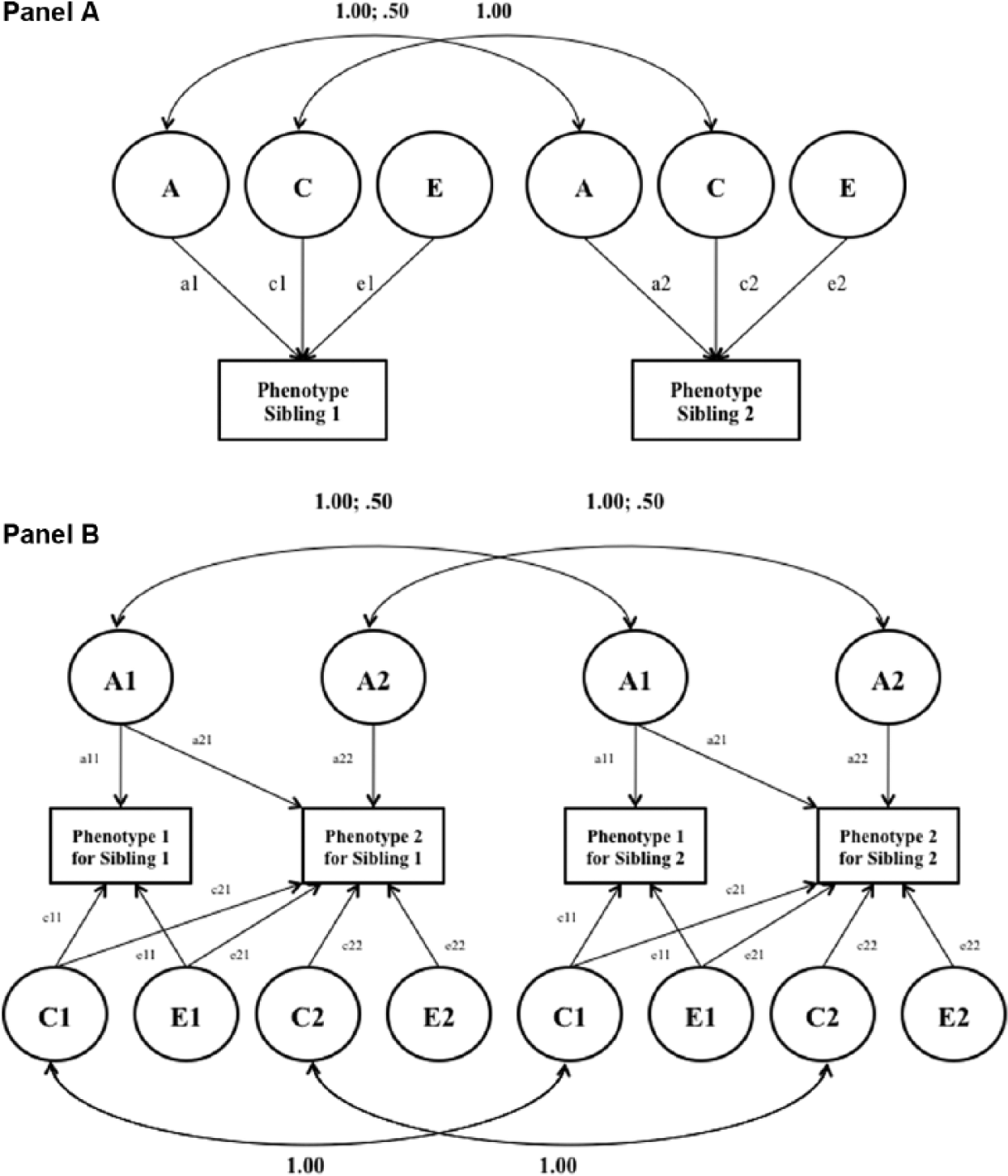
Diagram of the ACE and Cholesky models.
The third step to the analysis used a bivariate behavior genetic modeling technique known as the Cholesky model. This model is referred to as bivariate because it analyzes two outcomes at once. In this way, the Cholesky model is able to decompose variance in two outcomes simultaneously, as well as decompose the covariance between the two measures. To this point, the Cholesky model decomposed the correlation between football participation and violent behavior into genetic (A), shared environmental (C), and nonshared environmental (E) components that are common to both outcomes. In other words, the Cholesky model revealed the degree to which football participation and violent behavior covary due to a shared genetic etiology. A diagram of the Cholesky model, which was estimated using Mx (Neale et al., 2004), is presented in Panel B of Figure 1.
Two final points about the ACE and Cholesky models are worth noting before discussing the next step to the analysis. First, the ACE and Cholesky models were estimated along with a series of “nested” models. Nested models are models that constrain one or more of the paths (i.e., the A, the C, or both A and C) to zero. If a nested model was found to fit the data better than (or equivalent to) the full model, the nested model was chosen over the full model. What this necessarily means is that if a nested model is selected, then the path that was constrained to zero (and, therefore, omitted from the model) was not significantly contributing to the overall model fit. For instance, if an AE model is found to be the best-fitting model, then this could be interpreted to mean that shared environmental influences are inconsequential for explaining the variance or covariance of the model. Chi-square difference tests (i.e., Δχ2) and AIC fit statistics were consulted to determine the best-fitting model. Second, the threshold versions (Derks, Dolan, & Boomsma, 2004; Neale & Maes, 2004) of the ACE and Cholesky models were estimated due to the dichotomous coding of football participation and the violence indicator.
The fourth step to the analysis estimated the influence of football participation on violent behavior after genetic influences had been controlled. To control for genetic influences, we used the MZ difference score approach (Beaver, 2008; Plomin et al., 2008). Because MZ twins share 100% of their DNA, they cannot differ due to genetic differences. The corollary of this point is that the only reason MZ twins should differ on a phenotype is because they experience different environments. Thus, to the extent that football participation and violent behavior are causally related, MZ twins who are involved in football should be more violent than their co-twin who is not involved in football. To perform the analysis, cross-sibling difference scores were created for the football participation variable and the violence indicator variable. Thus, respondents were coded −1 = respondent not involved in football/violence but co-sibling was, 0 = neither respondent nor co-sibling were involved in football/violence or both respondent and co-sibling involved in football/violence, or 1 = respondent involved in football/violence but co-sibling was not. Next, the violence indicator difference score was regressed on the football participation difference score. A positive regression coefficient indicates that the respondent who was involved in football was more likely to be involved in violent behavior as compared with his or her co-sibling who was not involved in football.
Findings
Presented in Table 1 are the results from the logistic regression analysis where the violence indicator variable is used as the dependent variable and the other variables are used as covariates. Most important was the coefficient (i.e., the odds ratio) for the football participation variable. As shown in the table, the odds ratio was positive and statistically significant. The odds ratio revealed that respondents who were involved in football were 37% more likely to report being involved in violence than those who did not play football.
Logistic Regression of the Violence Indicator on Football Participation and Covariates.
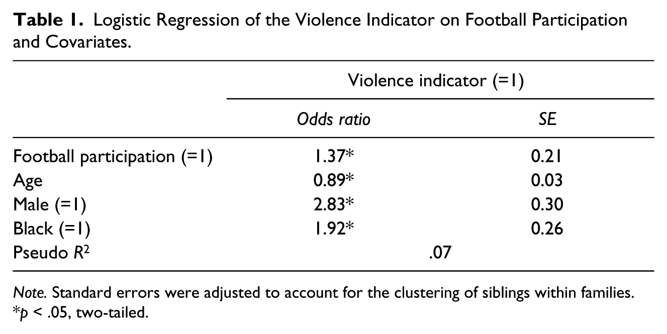
Note. Standard errors were adjusted to account for the clustering of siblings within families.
p < .05, two-tailed.
There were a number of females who admitted violent behavior and several indicated football participation so we chose to include these cases in the analyses. To be specific, 0.01% of females indicated football participation and 57.14% of those females also admitted to violence. Because sex determination is a genetic process (i.e., females carry two X chromosomes while males carry one X and one Y chromosome), because certain females reported football participation, and because females were involved in violence at a nontrivial rate (nearly 27% of all females reported violence, 57% of females participating in football admitted violence), we felt that it was important to include these cases in the analysis. Nonetheless, male sibling pairs were analyzed as a sensitivity check. These sensitivity analyses were estimated in recognition of two points. First, sex disparities in football participation are likely to result from genetic factors given that sex determination is a genetic process (as noted above). Second, although genetic factors will have an indirect effect on football participation via sex determination, it is also possible that cultural factors play a role in football participation (i.e., football is more popular in certain areas and females may be encouraged to participate in some areas but not others). Thus, the sensitivity analyses were important to consider.
When male participants were analyzed as a sensitivity analysis, the same substantive results were observed (Football participation odds ratio = 1.36, p < .05), indicating that the inclusion of females did not affect the logistic regression parameter estimates presented in Table 1. We report the results from male sensitivity checks for all analyses that follow.
The next step to the analysis was to estimate the genetic and environmental influences on football participation and the violence indicator.
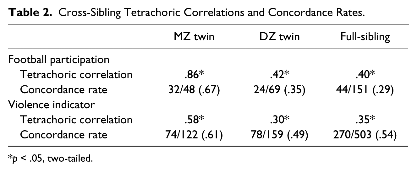
As noted above, tetrachoric correlations and concordance rates were observed first. These statistics are reported in Table 2. Turning first to the tetrachoric correlation for football participation, MZ twins had a cross-twin correlation of .86 (p < .05), which was higher than the tetrachoric correlation observed for DZ twins (r = .42, p < .05) and FS (r = .40, p < .05). A similar pattern emerged when the concordance rate was analyzed. As shown in the table, the concordance rate was .67 for MZ twins, .35 for DZ twins, and .29 for FS. Substantively similar results were gleaned from the tetrachoric correlations and concordance rates for the violence indicator variable. To be specific, MZ twins were more similar in their violent behavior (r = .58, p < .05) than DZ twins (r = .30, p < .05) and FS (r = .35, p < .05). The concordance rates revealed a substantively identical pattern of results. Taken together, these findings suggest that football participation and involvement in violent behavior are, at least partially, influenced by genetic factors. The next step to the analysis was to analyze exactly how much of the variance in football participation and violence was attributable to genetic, shared environmental, and nonshared environmental factors.
Cross-Sibling Tetrachoric Correlations and Concordance Rates.
p < .05, two-tailed.
To estimate the degree to which football participation and involvement in violence were influenced by genetic and environmental factors, the ACE model was analyzed. The ACE model results, along with three nested models, are presented for football participation and the violence indicator in Table 3. In both cases (i.e., for football participation and for the violence indicator), the AE model was the best-fitting model, meaning that shared environmental influences accounted for none of the variance in these models. In terms of football participation, the AE model revealed that approximately 85% of the variance was attributable to genetic factors. The remaining variance was attributable to nonshared environmental influences (15%). Similar results were gleaned from the ACE model analyzing the violence indicator. Specifically, the AE model best fit the data, and the results suggested that genetic factors explained the majority of the variance (62%) with the nonshared environment capturing the remaining variance (38%).
ACE (Threshold) Decomposition Models for Football Participation and the Violence Indicator.
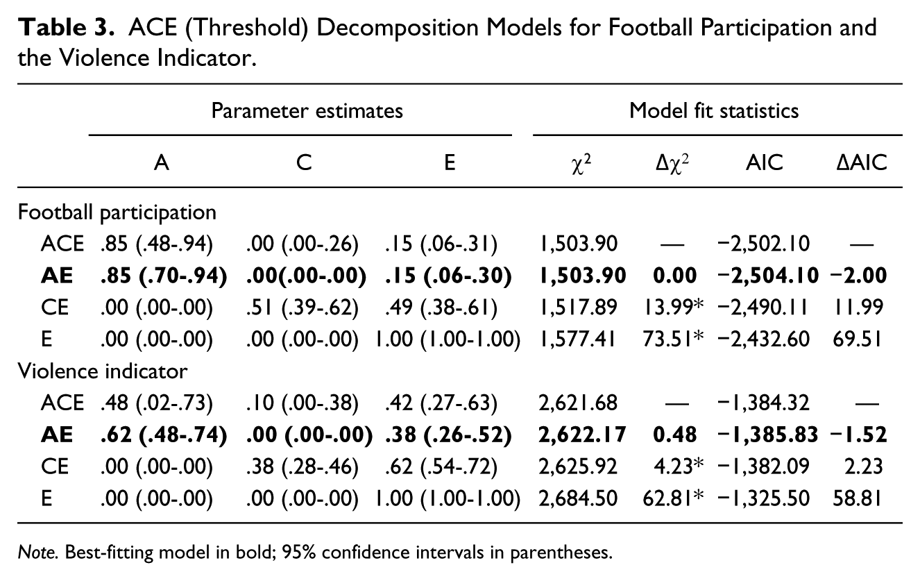
Note. Best-fitting model in bold; 95% confidence intervals in parentheses.
The ACE models were reestimated on the subsample of male sibling pairs as a sensitivity check. Under these conditions, the ACE model results indicated a genetic link to violence (A = .53, E = .47 in best-fitting model [Δχ2 = 0.00, Δdf = 1]) but suggested that the CE model (C = .69, E = .31 [Δχ2 = 2.31, Δdf = 1]) was the slightly better fit when football participation was analyzed (full ACE results were A = .39, C = .44, E = .17; for reference, the AE results were A = .88, E = .12 [Δχ2 = 5.05, Δdf = 1]). That the CE model is the best-fitting model for football participation when male sibling pairs are analyzed suggests that sex plays an important role in determining football participation—an unsurprising finding. These results, therefore, indicate that once the genetic effects that operate through sex determination are controlled (i.e., by analyzing only male siblings), the factors that explain variance in football participation are attributable to shared environmental factors (e.g., cultural influences) and nonshared environmental influences (e.g., physical size differences between siblings).
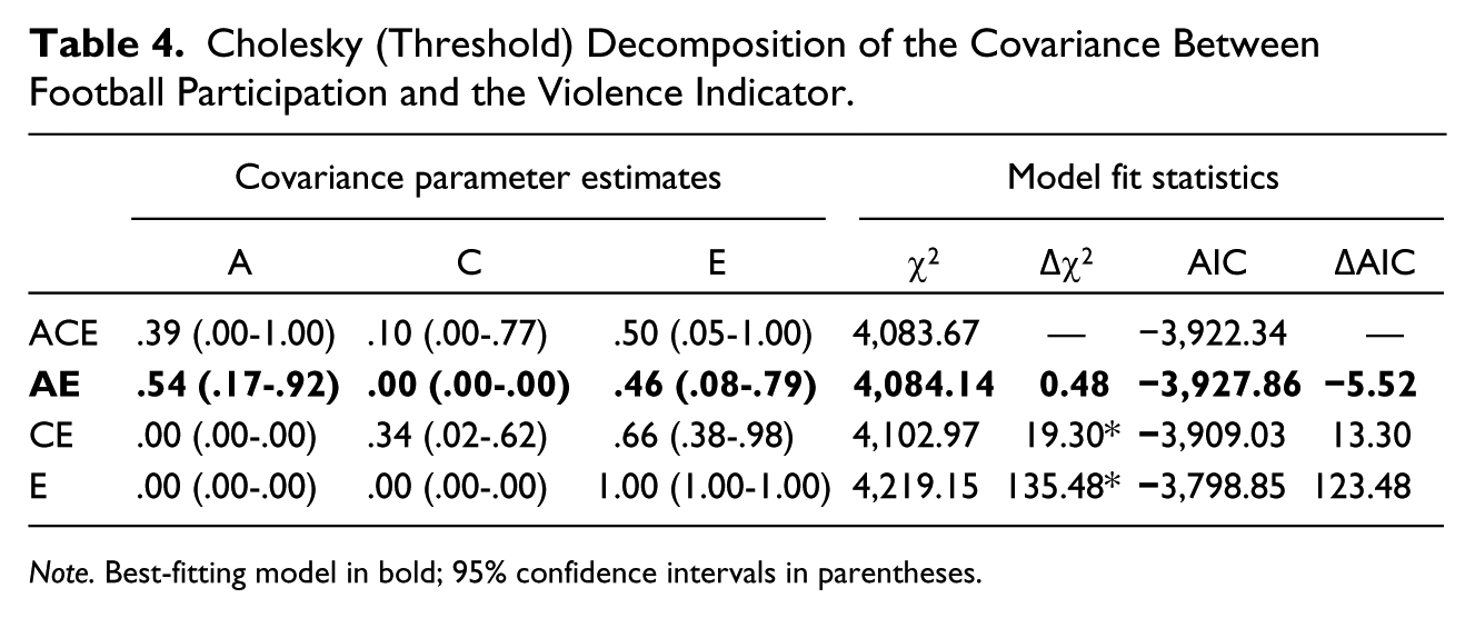
Thus far, the results have indicated that (1) football participation is associated with violent behavior (Table 1), (2) football participation is strongly influenced by genetic factors (Tables 2 & 3) and that much of this genetic influence is likely due to the genetic determination of sex (see sensitivity analysis results discussed above), and (3) violent behavior is strongly influenced by genetic factors (Tables 2 & 3). The extent to which football participation and violent behavior share a genetic etiology has yet to be examined. To do so, the Cholesky model was analyzed and the results from this model can be found in Table 4. As with the ACE model results, Table 4 presents parameter estimates and fit statistics for the full ACE model and the three nested models. The table reveals the AE model as the best-fitting model. The AE model results indicated that 54% of the association between football participation and violent behavior was attributable to genetic factors common to both outcomes. In other words, football participation and violent behavior share a genetic etiology, but this was not the only reason these two variables were correlated. The remaining covariance was explained by nonshared environmental factors (46%). When the Cholesky model was estimated on the male sibling pairs, the results were substantively similar to those reported here. To be sure, the AE model was the best-fitting model and the parameter estimates suggested that A = .32 and E = .68 (Δχ2 = 6.59, Δdf = 3).
Cholesky (Threshold) Decomposition of the Covariance Between Football Participation and the Violence Indicator.
Note. Best-fitting model in bold; 95% confidence intervals in parentheses.
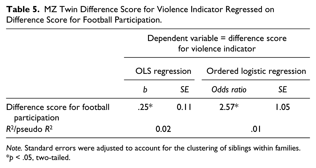
The final step to the analysis was to estimate the effect of football participation on violent behavior after genetic factors had been controlled. This is an important point to bear in mind because the Cholesky model revealed a genetic overlap for the two variables. Moreover, the violence indicator variable showed a large genetic influence, meaning that any variable used to predict involvement in violence may be (partially) spurious owing to uncontrolled genetic factors. Thus, not controlling for genetic influences on violent behavior may work to inflate the association between football participation and violence. To control for genetic influences on violent behavior, the MZ difference score method was used, and the results are presented in Table 5. As shown in the first two columns of Table 5, when the violence indicator difference score was regressed on the football participation difference score, OLS estimates suggested that football participation was correlated with violence. Interpreting these results is slightly different than a standard OLS model. This finding indicates that respondents who were involved in football were more likely to be involved in violence as compared with their co-sibling who was not involved in football. Because the dependent variable only included three categories (i.e., −1, 0, and 1), an ordered logistic regression model was estimated to confirm the OLS results. These findings are presented in the last two columns of Table 5. The substantive results garnered from the ordered logistic regression model are identical to those gleaned from the OLS model. Finally, when the models presented in Table 5 were reestimated on the male subsample, the substantive results were unchanged (OLS coefficient estimate = .23, p = .05; ordered logistic odds ratio = 2.21, p = .05).
MZ Twin Difference Score for Violence Indicator Regressed on Difference Score for Football Participation.
Note. Standard errors were adjusted to account for the clustering of siblings within families.
p < .05, two-tailed.
Discussion
Given the amount of media attention that has been devoted to high-profile athletes engaging in various forms of crime and violence (Benedict, 2004; Benedict & Yaeger, 1998; Otto, 2009), there has been a line of research examining whether there is indeed an association between playing sports and violent behaviors (e.g., Blumstein & Benedict, 1999; Crosset et al., 1995; Curry, 1998; Kreager, 2007; Otto, 2009). Although the results of these studies have been mixed depending on the sample analyzed and the types of sports examined, one of the more consistent findings to emerge from the literature is that adolescents who participate in football are more violent than youth who do not play sports or who play noncontact sports. The current study used this finding as a springboard to examine the genetic and environmental mechanisms that might be able to explain the association between playing high school football and involvement in violent behaviors. The findings provided partial support for three key explanations of why there is covariation between participating in high school football and violence.
First, to estimate the extent to which genetic and environmental factors are responsible for selection into playing football, univariate twin models were estimated. The results of these models indicated that 85% of the variance in football participation was attributable to genetic factors, and the remaining 15% was the result of nonshared environmental factors. Shared environmental influences explained none of the variance in football participation. These findings provide strong evidence suggesting that the decision to participate in high school football is scripted in large part by genetic factors. This genetic effect appears to work primarily through sex determination because the variance in football participation was attributable to shared and nonshared environmental factors when male sibling pairs were analyzed (see sensitivity results discussed in text). These findings, when juxtaposed against the findings from the full sample, reveal that football participation is the result of a complex arrangement of genetic factors (that likely work via sex determination) and cultural influences that affect a youth’s willingness to engage in contact sports such as football. Given that participating in high school football is largely influenced by genetic factors in the full sample, this necessarily suggests that future research examining the potential casual effect of sports on antisocial outcomes must control for genetic propensities; failure to do so would leave the statistical models misspecified and the findings generated from these models to be biased. Fortunately, samples such as the Add Health include sibling pairs allowing for genetically informative statistical models, which will allow for more accurate and reliable parameter estimates for sports variables, such as participating in football.
The second mechanism that was examined in the current study was the shared etiology explanation. According to this explanation, the factors that are causing football participation are also causing violent behavior. For this explanation to have merit, variance in football participation and violent behavior must be due to at least some of the same factors. The results of the univariate twin models provide support for this possibility as football participation and violence are influenced by genetic and nonshared environmental factors. This leaves open the opportunity for genetic factors, nonshared environmental factors, or some combination of the two, to explain at least part of the covariance between football participation and violence. A bivariate Cholesky decomposition model was estimated to directly test the shared etiology explanation. The findings from this model indicated that 54% of the covariance between football participation and violence was due to common genetic factors, and the remaining 46% was the result of common nonshared environmental influences. To our knowledge, this is the first study revealing that part of the overlap between playing high school football and adolescence violence is the result of genetic influences.
The last explanation that was examined in this study was the causal effect explanation that posits that participating in football causes youth to become more violent. To take into account the potential confounding effects of genetic factors, we estimated an MZ-twin-difference-score model that holds genetic influences constant. The results of this model revealed a statistically significant influence of football participation on violent behavior. Because the MZ-difference-scores model has been identified as a strong research design capable of addressing salient sources of confounding (Vitaro, Brendgen, & Arseneault, 2009), this finding represents some of the most convincing evidence to date that participating in high school football has some causal effect on violence.
Study Limitations
The analyses conducted in this study provide evidence in favor of all three explanations of the association between high school football participation and violent behavior. Even so, there are a number of limitations that need to be addressed in future studies. First, we were only able to assess the associations between genetics, football participation, and violence at a single point in time. Prior research, however, has revealed that genetic influences on participating in sports and violent behavior vary across different periods of the life course (Stubbe et al., 2005). As a result, it is quite possible that the estimates reported here would differ at various ages. Future research should address this possibility by examining the longitudinal association between sports and violence by collecting data on these measures at multiple time points in adolescence. Doing so would provide a more rigorous analysis of the cross-sectional and longitudinal influence of sports on subsequent violent behaviors.
Second, the current study only examined participation in one sport—football—and only at one level—high school. The decision to focus only on football was due to the fact that it was the only contact sport that had sufficient base rates to examine within the genetically informative analysis. It would be interesting to examine a broader range of sports and the differential associations that they might have with violence. Moreover, it would be important to examine whether participation in sports at different levels—such as high school, college, and even professionally—are associated with violent behaviors.
Third, only violent behavior was examined as an outcome measure. We focused on violence because prior research has shown a statistical link between football participation and violence (Kreager, 2007), but it would be important to examine whether other outcomes, including drug and alcohol use, would show a similar pattern of results as those reported with violence. Relatedly, the measure of violence used in the current study was dichotomized. Our decision to use a dichotomous, as opposed to continuous, measure of violence was driven by the distribution of the violence measure, wherein more than 60% of the sample reported no acts of violence. Although previous research has used dichotomous measures of violence (Kreager, 2007 analyzed a dichotomous measure of involvement in serious fighting, a variable included in our violence indicator), it is possible that a different pattern of results would emerge when using alternative measures of violence. Future research is needed addressing these shortcomings to determine whether the current findings are robust.
Last, there are some potential limitations and shortcomings with twin/sibling-based research designs. Of particular salience is whether the findings from these studies are generalizable to the larger population of nontwins/siblings. In a recent article, Barnes and Boutwell (2013) examined this possibility by comparing twins from the Add Health to the nationally representative sample of Add Health respondents across a range of demographic and behavioral measures. The results of their analysis revealed that the two samples were largely similar, suggesting that findings from the kinship pairs of the Add Health would generalize to the larger population. In addition, the methodology used in the current study only provides estimates of variance explained and thus does not provide any information as to the precise genes or the precise nonshared environments that are involved in explaining the variance. Based on previous research (Beaver, 2013), it would stand to reason that genes involved in neurotransmission and environments that capture peer influences would be integral to understanding the link between football participation and violence. To more fully address this possibility, research using different methodological approaches is needed to identify the genes and nonshared environments that might link sports to violent behaviors.
While there can be little doubt that participating in sports can have prosocial effects on adolescents, including an emphasis on the importance of teamwork and persistence, analysis of sibling pairs from the Add Health also indicates that there are negative effects that are evident as well. Future research is needed to continue to examine the various outcomes associated with participating in high school sports, but as our findings indicate, such research must use genetically informative research designs or it may produce biased findings that might result in distorted views about high school sports and athletes.
Footnotes
Acknowledgements
Special acknowledgment is due to Ronald R. Rindfuss and Barbara Entwisle for assistance in the original design.
Authors’ Note
Persons interested in obtaining data files from Add Health should contact Add Health, Carolina Population Center, 123 W. Franklin Street, Chapel Hill, NC 27516 -2524 (
Declaration of Conflicting Interests
The author(s) declared no potential conflicts of interest with respect to the research, authorship, and/or publication of this article.
Funding
The author(s) disclosed receipt of the following financial support for the research, authorship, and/or publication of this article: This research uses data from Add Health, a program project designed by J. Richard Udry, Peter S. Bearman, and Kathleen Mullan Harris, and funded by Grant P01-HD31921 from the Eunice Kennedy Shriver National Institute of Child Health and Human Development, with cooperative funding from 17 other agencies. No direct support was received from Grant P01-HD31921 for this analysis.