
Abstract
This research fills the gap in the tourism literature on the impacts of country stability—including political, financial, and economic—on tourism development (i.e., international tourist arrivals, international tourism revenues, and travel and leisure sector returns). To account for possible asymmetric and nonlinear relationships among variables, we apply a new method of moment quantile regression, by using panel data from 106 countries spanning the period 2006–2017. From a global perspective, the empirical results indicate that higher country stability generally leads to higher tourism development, while there is no salient influence of financial stability on travel and leisure sector returns. This suggests that the effects of country risk ratings are mostly nonlinear across different tourism development quantiles. Additionally, different components of risk rating scores have diverse impacts on tourism development. The findings mean that policy makers should consider their tourism condition when setting country stability strategies.
Keywords
Introduction
It is widely acknowledged that the most important sector in the path of a country’s economic development is travel and leisure. According to the World Travel and Tourism Council (WTTC) (2019), in 2018 it contributed US$8.8 trillion to the global economy, created 319 million jobs, and increased global GDP by 10.4%. Travel and leisure, the second-fastest growing sector in 2018 only marginally behind manufacturing, certainly has had an impressive impact on the world economy (WTTC 2019). In fact, the sector is now the most noteworthy service sector globally, becoming an agent of economic growth and development that has been broadly adopted and officially sanctioned by most countries (Lee and Chang 2008; Lee, Olasehinde-Williams, and Akadiri 2020). Therefore, the factors that are influencing the flow of travelers around the world, such as destinations’ institutional environments, continue to affect travelers’ behaviors. With nearly all countries looking to attract international visitors, the significant contribution of the tourism industry and many economies’ increased dependency on its revenues warrant a more detailed analysis of the underlying factors and trends that drive this industry.
Tourists are generally regarded as longing for relaxing and unconcerned holiday making and therefore are sensitive to events of violence at holiday destinations, because such events can jeopardize their holiday goals (Neumayer 2004). Ankomah and Crompton (1990) suggest that a major consideration in a potential traveler’s decision to visit any foreign destination is that country’s political stability and general internal security conditions. Ma and Hassink (2014) pinpoint that new pathways for tourism are created based on preexisting tourism attractions and institutional environments, for which the latter include the set of rules, laws, regulations, customs, practices, and procedures that influence human behavior within an economic system (Martin and Sunley 2006).
Based on the institutional environments theory, most studies in the related literature discuss the impact of political risks on tourism. For example, Hall and O’Sullivan (1996) find that perceptions of political instability and violence profoundly affect tourist visitation. Eilat and Einav (2004) note that political risk of a destination country is a crucial consideration in the tourism economy. Endo (2006) depicts that political and/or economic risks significantly affect foreign direct investment in tourism. Ghalia et al. (2019) find that the prevalence of political turbulence can cause a significant number of service providers and operators in the tourism sector to suspend business activities.
Although the tourism literature has extensively analyzed the impact of political risk, three components of country risk rating (CR) (economic, financial, and political) have not received appropriate attention. Specifically, knowledge is limited as to whether all types of CR exhibit similar impacts on tourism development. Country risk assessment evaluates economic, financial, and political factors and their interactions in determining the risk associated with a particular country (Chiu and Lee 2020). As tourism is a service export, tourism earnings are accommodated in the current account balance, or one of the variables among a country’s economic and financial risks. Therefore, higher tourism earnings lead to a higher current account balance, higher economic and financial stability, and subsequently country stability. The higher the country stability is, the higher is the likelihood that a country will repay its obligations to its foreign lenders/investors, and the higher the creditworthiness a country has (Hoti, McAleer, and Shareef 2007). Overall, the creditworthiness of a country with an increasing stability results in higher inflows of foreign capital and investment, which in turn assist in that country’s economic development (Hoti, McAleer, and Shareef 2007).
Country risk (country instability) may be prompted by a number of country-specific factors or events (Hoti and McAleer 2004; Chiu and Lee 2020). Additionally, economic and financial risks include factors such as a sudden deterioration in the country’s terms of trade, rapid increases in production costs and/or energy prices, and unproductively invested foreign funds (Nagy 1988). The lack of empirical evidence on the topic is particularly surprising given the growing awareness of country risk assessments, as well as the close link among country risks and economic activities (Hoti 2005; Sari, Uzunkaya, and Hammoudeh 2013; Liu, Hammoudeh, and Thompson 2013; Brückner and Gradstein 2015). Risk affects visitors and investors alike (Sequeira and Nunes 2008). For instance, country risk may be present as a result of various unexpected and random events that can affect consumer decisions, such as the Tiananmen Square event, 9/11 terrorist attacks, the SARS outbreak, and the Bali bombing in 2002 (Hoti, McAleer, and Shareef 2007). Therefore, the influence of country risks (country instability) on tourism development needs to be appreciated in order to execute optimal economic management and policy decision regarding tourism growth and country risk.
This article extends the existing literature on the rapidly growing tourism field by examining how different dimensions of country risk ratings (economic, financial, and political) affect tourism development (i.e., international tourist arrivals, international tourism revenues, and travel and leisure sector returns) in an international framework. We employ International Country Risk Guide (ICRG) data and a new panel quantile regression to assess whether the influences of country stability are positive on tourism development under different tourism distributions over the period 2006–2017. This topic deserves a more in-depth investigation, because the risks of institutional environments, such as political stability, economic volatility, and financial unrest, influence tourism development, thereby altering a country’s economy.
The contributions of this article are threefold. First, to our knowledge, this study provides initial international evidence regarding the effects of multifaceted country risk (i.e., economic, financial, and political risks) on tourism development. Second, considering the nonlinear and/or asymmetric relationship between country risk (country instability) and tourism development, we take advantage of a new panel quantile regression (i.e., method of moment quantile regression [MMQR]) approach proposed by Machado and Silva (2019) to identify how country risk ratings affect the entire conditional distribution of tourism development. The moment estimation offers a flexible tool to assess panel quantile regression, especially when the parameter estimations are hard or even impossible (e.g., a model with endogenous effects and a panel data model with individual effects), thus generating reliable and robust results for policy formulations (Guo, You, and Lee 2020). This article is a pioneering tourism study that uses MMQR to beneficially complement the present literature.
Third and finally, we check the nonlinear relationship between country risk ratings and tourism development across different quantiles of tourism data, which allows us to identify different responses of tourism development to country risk ratings at varying points of the conditional development distribution. The findings suggest that countries with different levels of tourism development can employ diverse strategies to improve their tourism economy. This new empirical evidence from our study provides a more complete picture of the determinants of tourism development and indicates that government policies are unlikely to succeed equally across countries under different development levels.
Our research is organized as follows. The second section briefly reviews the literature and hypotheses. The third section illustrates the research methodology. The fourth section analyzes the empirical results obtained and presents a discussion. The final section concludes the study.
Literature Review and Hypothesis Development
Hoti and McAleer (2004) state that country risk has become a topic of major concern for the international financial community over the last two decades. Using survey-based country credit ratings, Erb, Harvey, and Viskanta (1995, p. 76) find that lower country risk ratings (i.e., higher country risks) are associated with higher average equity returns for most countries. Employing three country risk ratings from ICRG—political, economic, and financial risk ratings—Erb, Harvey, and Viskanta (1996) further show that financial and economic risks have the most explanatory power on expected equity returns, while political risk has the least. Diamonte, Liew, and Stevens (1996) find that political risks have a greater influence on the expected market returns in emerging markets than in developed markets. Sari, Uzunkaya, and Hammoudeh (2013) demonstrate that political and financial risk ratings significantly and positively affect equity market movements in the short run for Turkey. Liu, Hammoudeh, and Thompson (2013) examine the asymmetric relationship between stock market indices and three country risk ratings and suggest that there is asymmetry in the long-run relationship in response to positive and negative shocks for each country. We therefore observe abundant findings on different country risks-return relations in the financial filed.
While the aforementioned literature is critical to our understanding of the risk–returns relation, there is a growing awareness on the connection between country risks and tourism. Tourism, as a service industry, seems to require an institutional environment that is fundamentally different from that common in resource peripheries (Carson and Carson 2011). The institutional environment may be understood as the set of rules, laws, regulations, customs, practices, and procedures that influence human behavior within an economic system (Martin and Sunley 2006). A favorable institutional environment includes high levels of local social capital as well as explicit formalized institutions that support tourism (Carson and Carson 2011). Ma and Hassink (2013) note that the institutional environment is considered to be a source of constraining or enabling influence on the evolution of tourism sectors and products. Additionally, Ma and Hassink (2014) pinpoint that new pathways for tourism-related products and firms are created based on preexisting tourism attractions and institutional environments. Therefore, governments in countries that are dependent on tourism should strive to put in place sound institutions and a stable political environment, which might enable them to reap further gains from the tourism sector.
Using ICRG country risk ratings, Shareef and Hoti (2005) explore the relations between small island tourism economies (SITEs) and country risk ratings and find that the tourism economic growth rate positively correlates with risk ratings in only 13 of the 24 cases, concluding that the tourism economic characteristics of SITEs should be examined more carefully in the country risk literature. Hoti, McAleer, and Shareef (2005) find that the relation between tourism and country risk is not statistically adequate for all their sample cases. Saha and Yap (2014) note that terrorism increases tourism at a very low to moderate level of political instability, but after a certain threshold level it substantially lowers the value of tourist arrivals and tourism revenue. Schnusenberg, Madura, and Gleason (2007) also present that stock market valuations are not affected by changes in country ratings. Therefore, the relationships between country stability and tourism developments are not always positive or negative, indicating an asymmetric or nonlinear relationship possibly exists across different tourism development quantiles.
The finding of a linear or nonlinear relationship between country risks (country instability) and the tourism literature is still inconsistent. For example, Neumayer (2004) states that conflicts and other politically motivated violent events negatively affect tourist arrivals. Yap and Saha (2013) suggest that although country risk is a robust and significant determinant of tourist arrivals and tourism revenues of countries, an increase in the corruption index does not have an adverse influence on tourist arrival numbers, particularly for those countries that have historical and natural heritage. This suggests a possible nonlinear and/or asymmetric relationship between tourism development and country risk. Saha and Yap (2015) show that corruption has a significant nonlinear effect on tourism demand. Accounting for asymmetry in this context is critical as investors’ reaction to good versus bad news regarding political or economic developments can lead to markedly different effects on the local stock market (Ben Nasr et al. 2018). If one argues that investors overreact to bad news and not necessarily to good news, then such an asymmetric reaction may open up arbitrage possibilities for investors depending on the direction of a firm’s credit rating change, and this can translate into significant arbitrage profits for investors (Ben Nasr et al. 2018).
Employing data from 139 countries, Saha and Yap (2014) show that countries experiencing high levels of political risk witness significant reductions in their tourism businesses. Cervelló-Royo, Peiró-Signes, and Segarra-Oña (2016) state that since the link between tourism and economic growth is not automatic, a country must possess certain characteristics in order for this link to arise and be sustainable through time. Among the characteristics the authors list, environmental and sustainable policies, the existence of hard and soft infrastructure, and economic and financial indicators play key roles, and thus policy makers should consider their impacts. However, Cervelló-Royo, Peiró-Signes, and Segarra-Oña (2016) focus on environment awareness, which is different from our aim. Muzindutsi and Manaliyo (2016) note that political risks have a long-run effect on factors fostering tourism flows for destination countries. Consequently, little is known about the three individual impacts of economic, financial, and political risk ratings (ECO, FIN, and POL) on tourism development factors (i.e., TA, TR, and SR) with respect to international empirical evidence. We develop the following hypotheses to generalize the relationship of country risks with international tourist arrivals, international tourist revenues, and travel and leisure sector returns, respectively.
Hypothesis 1a: Economic stability has a positive effect on international tourist arrivals.
Hypothesis 1b: Financial stability has a positive effect on international tourist arrivals.
Hypothesis 1c: Political stability has a positive effect on international tourist arrivals.
Hypothesis 2a: Economic stability has a positive effect on international tourism revenues.
Hypothesis 2b: Financial stability has a positive effect on international tourism revenues.
Hypothesis 2c: Political stability has a positive effect on international tourism revenues.
Hypothesis 3a: Economic stability has a positive effect on travel and leisure sector returns.
Hypothesis 3b: Financial stability has a positive effect on travel and leisure sector returns.
Hypothesis 3c: Political stability has a positive effect on travel and leisure sector returns.
Hypothesis 4: The relationship between country stability and tourism varies at different quantiles of the tourism distribution.
Methodology
Data
We employ ICRG risk rating score data constructed by the Political Risk Services Group, which comprises three subcategories: economic (ECO), financial (FIN), and political (POL) risk ratings. The three indices evaluate a country’s political stability and ability to finance its official, commercial, and trade debt obligations on a comparable basis. Political risk compounds the degree of political uncertainty in a given country. Economic risk is a measure of assessing a country’s current economic strengths and weaknesses. The overall aim of financial risk is to provide a measure of a country’s ability to finance its official, commercial, and trade debt obligations (Hayakawa, Kimura, and Lee 2013; Lee, Lee, and Lien 2019, 2020). Except for the political risk rating scoring from 0 to 100, financial and economic risk ratings both range from 0 to 50. Each of the five economic and financial components account for 25%, while the 12 political components account for 50% of the composite risk rating (Hoti, McAleer, and Shareef 2007). The ICRG rating system comprises 22 variables representing three major components of country risk: economic, financial, and political (Hoti 2005). The country risk increases as the rating declines. In other words, a lower (higher) given rating implies a higher (lower) associated risk. Thus, an ascending rating score indicates a descending degree of risk (Lee and Lee 2018; Chiu and Lee 2020).
ICRG risk ratings have been cited by experts at the International Monetary Fund, World Bank, United Nations, and other international institutions as a standard against which other ratings are measured. ICRG has also been acclaimed by publications such as Barron’s and the Wall Street Journal for the strength of its analysis and rating system (Suleman, Gupta, and Balcilar 2017). As tourism is a service export, tourism earnings are accommodated in the current account balance, or one of the 22 variables in the ICRG rating system. Therefore, higher tourism earnings lead to a higher current account balance as well as greater economic and financial stability.
Our sample covers 106 countries/regions over 2006–2017, which is an unbalanced panel due to data availability. Table A1 provides the sample countries/regions, and Table A2 gives all detailed definitions and sources of the variables in the empirical analysis. Our main dependent variables to proxy tourism development are TA, TR, and SR, which are the widely used measures for tourism development in the empirical literature. For example, employing international tourism revenues, Belloumi (2010) explores the relationship among tourism revenues, real effective exchange rate, and economic growth. Eugenio-Martin, Martín Morales, and Scarpa (2004) use the number of tourist arrivals to study the relationship between the number of tourist arrivals and economic growth. Chen (2011) and Cave, Gupta, and Locke (2009) employ tourism sector stock returns to evaluate the performance of supply-side investments in the tourism industry. Following the abovementioned studies, the three dependent variables of tourism development used herein are log of international tourist arrivals (TA), log of international tourism revenues (TR) from the World Bank database, and yearly travel and leisure sector prices from the DataStream database. Sector returns (SR) are estimated by (Pt − Pt −1) / Pt −1, where Pt is the adjusted closing price at time t in US dollars. Because the latest data of TA and TR are for the year 2017, our empirical study uses the 106 countries/regions possessing tourism and risk ratings.
We also include a number of control variables in the MMQR models to strengthen our empirical results. According to the tourism demand model, Lim (2006) pinpoints that the five most common explanatory variables used in tourism demand models are income (GDP), relative prices (i.e., the ratio of prices in the destination country to prices in the origin country), transportation costs, exchange rates, and trend. Saha and Yap (2014) state that governments in high-income countries can afford to invest funds to build up and maintain infrastructure for the tourism industry, which in turn attract more tourists, expecting that high income increases demand for tourism. Castro-Nuño, Molina-Toucedo, and Pablo-Romero (2013) also show a positive relationship between GDP and tourism. CPI is commonly used as a proxy to count relative price (Wang 2009). While Aki (1998) finds a negative relationship between tourist arrivals and relative prices, Chen (2010) notes that a host country’s ΔGDP does not have a significant influence on hotel stock performance.
Chang and McAleer (2012) find in the case of Taiwan that the exchange rate typically has an expected negative effect on tourist arrivals to Taiwan. Chao et al. (2013) examine how currency depreciation affects the prices of inbound tourism, illustrating that the exchange rate has a dominant effect on the amount of tourists who enter a country. Consequently, domestic currency depreciation may harm the revenue of inbound tourism (Chao et al. 2013). Martins, Gan, and Ferreira-Lopes (2017) indicate evidence that an increase in GDP per capita (GDP), a depreciation in the national currency (EXG), and a decline of relative domestic prices (RP) all help boost tourism demand. Fereidouni and Al-mulali (2014) present the existence of a long-run, bidirectional causal relationship between FDI and international tourism. Craigwell and Moore (2008) find that FDI provides much needed capacity for countries and therefore allows them to expand their tourism product. Inchausti-Sintes (2015) denotes that tourism promotes economic growth and reduces unemployment. Chatziantoniou et al. (2013) show that oil-specific demand shocks exercise a significant negative impact on tourism sector equity returns.
Following Webster and Ivanov (2014) and Albaladejo, González-Martínez, and Martínez-García (2016), this study takes the natural logarithm of each variable in the following analysis (except for global crisis dummy [CRISIS] and SR, which have negative values) in order to avoid favoring countries with large populations, economies, tourism sectors, or per capita GDP, as well as coefficients that may be interpreted as presenting elasticities. All data are gathered in US dollars. We thus consider the influence of economic factors by including RP (relative prices), EXG (official currency exchange rate), FDI (foreign direct investment), GDP (GDP per capita), OIL (crude oil price ratio), and UMP (unemployment, total % of total labor force). Among the six macroeconomic factors, five of them are from the World Bank database, while OIL is from http://oilpirce.com. Additionally, as tourism involves discretionary income, it is anticipated during hard economic times that people may select to save cash for use on the basics of life such as food, shelter, and family necessities (Papatheodorou, Rosselló, and Xiao 2010). Therefore, according to Aizenman and Hutchison (2012), we set the global financial crisis period at 2008-2009 and examine this period using a CRISIS dummy.
In addition to a full-sample analysis, we also divide all observations into high- and low-country risk rating groups by the composite risk rating score of ICRG to explore whether the impact of country stability on tourism development is different by risk rating scores. Balli, Tsui, and Balli (2019) forecast visitor arrivals by controlling regional structural changes. Eugenio-Martín, Martín Morales, and Scarpa (2004) find that the nexus in the number of tourist arrivals and economic growth exists in developing countries, but not in developed countries. Therefore, to conduct robustness tests we divide the sample data into three subgroups: developing country, high- and low-country risks, as well as 36 countries in Europe.
Table A3 provides summary statistics of our main variables. We see from Table A3 that SR varies between −0.836% and 5.852% during the sample period, with the median being 0.023% and the average at 0.12%. The travel and leisure sector returns are positively skewed, suggesting that the tail on the right side of the probability density function is fatter than that on the left side. The kurtosis coefficients are greater than 33.024 for SR, indicating that the series have fatter tails. Moreover, the distributions are asymmetric. The Jarque-Bera (JB) statistics of all variables indicate departures from normality and display the existence of nonlinear portions in the data-generating process, thus providing further motivation to use panel quantile regression on the equations.
The average TR in log form is 8.031, and it ranges between 9.36 and 5.791, with a 0.486 standard deviation during the sample period. The average TA in log form is 6.957. Before estimation, the correlation matrix is checked to confirm that collinearity is not a problem. Table A4 displays that the Pearson correlations between tourism developments and country risk ratings are all positive, except for POL and SR. The correlation coefficients of country risk ratings and control variables are generally significant with each other. The negative associations here between EXG with TR and TA are consistent with Forsyth, Dwyer, and Spurr (2014) in that an increased exchange rate places intentional visits to Australia at a competitive disadvantage, reducing international leisure tourism demand. Though previous research has addressed a negative effect of oil prices on the tourism sector (e.g., Yeoman et al. 2007), OIL saliently and positively correlates to SR, implying a higher oil price does influence SR. The panel unit-root test results show a uniform conclusion that all variables are stationary in level. The probabilities for the Fischer-ADF and Levin, Lin, Chu (LLC) tests are computed using an asymptotic chi-square distribution in Table A5.
Models
Liu, Hammoudeh, and Thompson (2013) note a long-run asymmetric relationship between countries’ stock markets and their respective country risk ratings, depending on the direction of the shock as well as the specific type of risk. Chiu and Yeh (2017) identify that if one ignores the possibility that the tourism–economic growth nexus could be nonlinear, then the results of a linear model often cause bias due to using a false valuation method. The conventional ordinary least squares (OLS) method affords summary point estimations for the mean results of the explanatory variables. Focusing on the average effects may under- or overestimate the related coefficient estimates or may even fail to identify important relations (Binder and Coad 2011).
Ike, Usman, and Sarkodie (2020) explore the long-run effects of oil production on environmental pollution that is controlled for distributional heterogeneity by using the novel MMQR, which is useful for a more robust assessment of the empirical relationship and is proposed by Machado and Silva (2019). Using MMQR, Guo, You, and Lee (2020) analyze the impacts of affecting factors on CO2 emissions at various quantiles and control for diverse econometric challenges such as endogeneity and heterogeneity. Elheddad et al. (2020) employ MMQR to estimate models with fixed effects and models with endogenous explanatory variables. Because the inherent heterogeneity is usually higher under volatile market conditions, the relations between market returns and independent variables might vary across their conditional distributions (Badshah 2013). Based on the above discussion, we implement the models to mainly estimate whether country risks influence TA, TR, and SR by expanding upon the descriptive statistics in Table 1 and from testing equations (1), (2), and (3) via TA, TR, and SR as the dependent variables, respectively.


Estimates of the MMQR-Based International Tourist Arrival Models.
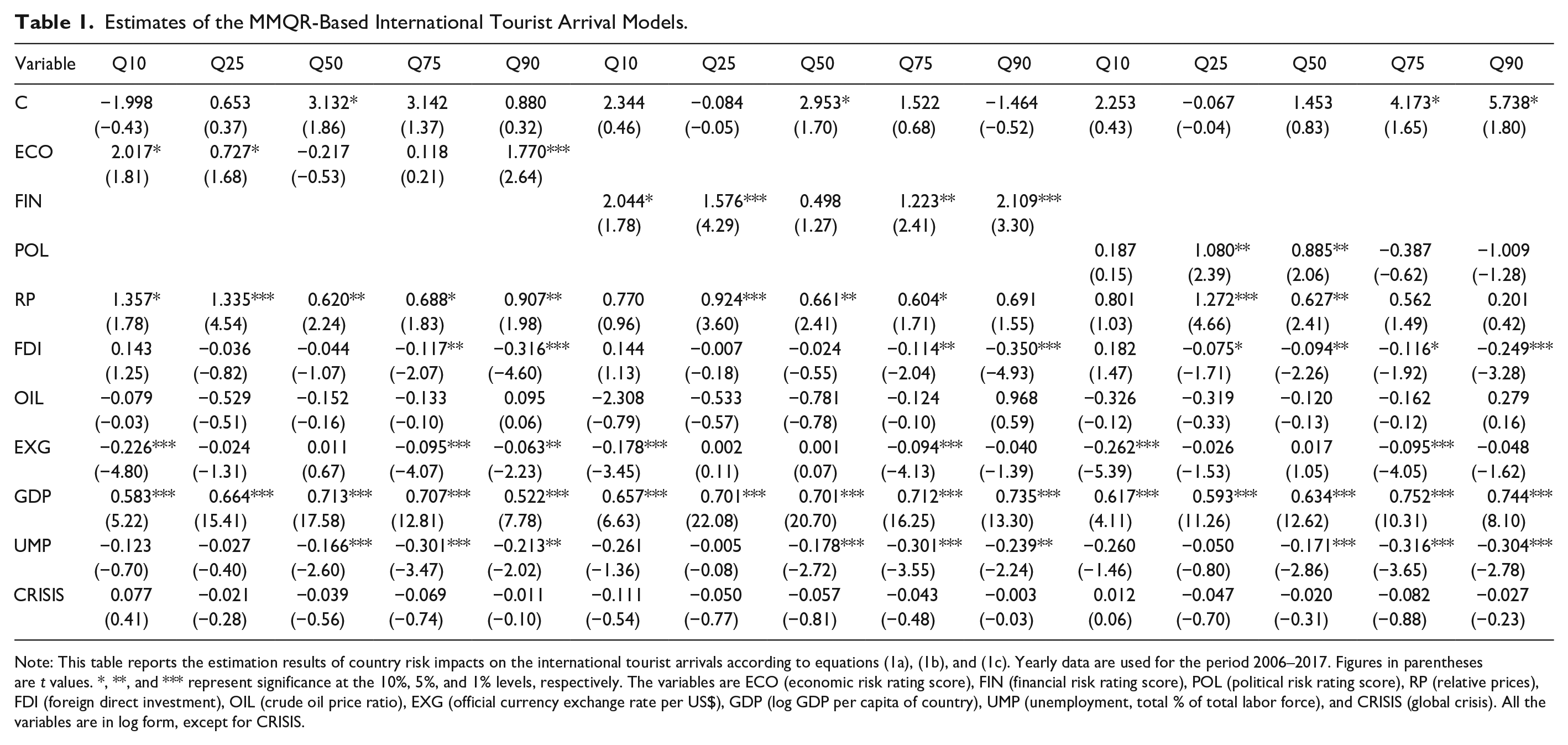
Note: This table reports the estimation results of country risk impacts on the international tourist arrivals according to equations (1a), (1b), and (1c). Yearly data are used for the period 2006–2017. Figures in parentheses are t values. *, **, and *** represent significance at the 10%, 5%, and 1% levels, respectively. The variables are ECO (economic risk rating score), FIN (financial risk rating score), POL (political risk rating score), RP (relative prices), FDI (foreign direct investment), OIL (crude oil price ratio), EXG (official currency exchange rate per US$), GDP (log GDP per capita of country), UMP (unemployment, total % of total labor force), and CRISIS (global crisis). All the variables are in log form, except for CRISIS.
We note here that
Equations (1) to (3) can answer the question of “whether country stability symmetrically affects tourism development.” However, it does not solve the problem if “country stability can affect tourism development differently for countries with different levels of tourism development.” From the viewpoint of policy making, it is more interesting to understand what happens in extreme cases. To answer these questions, quantile regression can be very useful. It is an extensive form based on the traditional regression and can offer a complete picture of a conditional distribution. For our study, this method helps obtain the full influences of country risk ratings across the entire distribution of tourism development. Furthermore, this model is robust to outliers, heteroskedasticity, and skewness (Koenker and Hallock 2001).
We write the equation as follows:

where 0 <
More and more researchers are concerned about addressing this problem by including quantile regression with panel data in the tourism field (Lv and Xu 2017; Akron et al. 2020). Compared with time series data, the advantages of panel data comprise an increased amount of observations and corresponding variations, as well as a reduction of noise caused by individual time series regression (Westerlund, Narayan, and Zheng 2015). Thus, equation (4) is modified as the following panel quantile regression form:

While the literature has broadly examined the quantile regression model with panel data, the studies always assume that the individual effect is just a location shifter and does not affect the whole distribution. Even more imperative is that these approaches cannot process the model with endogenous variables. In order to solve these problems, Machado and Silva (2019) propose a new panel quantile regression model via moments. Following Machado and Silva (2019), we identify the following equation:

where

where

where
As with other panel quantile fixed effect approaches, one of the main problems in this method lies in the incidental parameters due to the abundant fixed effects adopted (Neyman and Scott 1948; Lancaster 2002). The estimated results are not consistent, in which case the quantity of cross-sectional units moves toward infinity, whereas the observations’ amount of per cross-sectional unit is fixed (Kato and Galvao 2010). To deal with this concern, one can utilize the sequential estimation procedure based on the method of moment quantile regression proposed by Machado and Silva (2019).
Results
Impacts of Country Risk Ratings on International Tourist Arrivals
Table 1 shows the estimation results of panel quantile regression based on the Machado and Silva (2019) approach with fixed effects. Table 1 reports the MMQR parameter estimates for the impacts of CRs on different TA at the 10%, 25%, 50%, 75%, and 90% levels. ECO (FIN) has a saliently positive effect on TA at lower and higher TA quantiles, while POL notably has positive effect at lower and intermediate quantiles. This indicates that increasing TA ECO and FIN (POL) is important for countries with lower- and higher- (intermediate-) levels of TA. In other words, when tourism activities develop to a certain high level, POL inverts to having no effects on country tourism development. Since a higher risk rating indicates lower country risk (more stability), the results suggest that countries with lower and higher (intermediate) TA quantiles benefit from higher ECO and FIN (POL). This runs in line with Dacin, Goodstein, and Richard Scott (2002) as well as Ritchie, Goeldner, and McIntosh (2003) in that institutional quality in potential destination countries is an important determinant of inbound tourism.
The three CRs show partially positive and significant relations with TA. The results partially support hypotheses 1a, 1b, and 1c in that ECO, FIN, and POL have a positive effect on international tourist arrivals for the majority of TA quantiles. Thus, the estimation results in Table 1 clearly imply that the effects of different CRs on TA are heterogeneous. The corresponding results appear in Figure 1, which allows us to observe the diverse change patterns in the coefficients of CRs with respect to different quantiles. The solid line shows the point estimation results at different quantile levels, and the shaded bands represent the corresponding 90% confidence intervals. In each subfigure of Figure 1, coefficient estimates of CR are on the y-axis, while the quantile index of TA is on the x-axis. As can be seen, the intensity of the effects varies across the entire spectrum of quantiles. The estimation and testing results indicate that the effects of different CR on TA are quite heterogeneous.
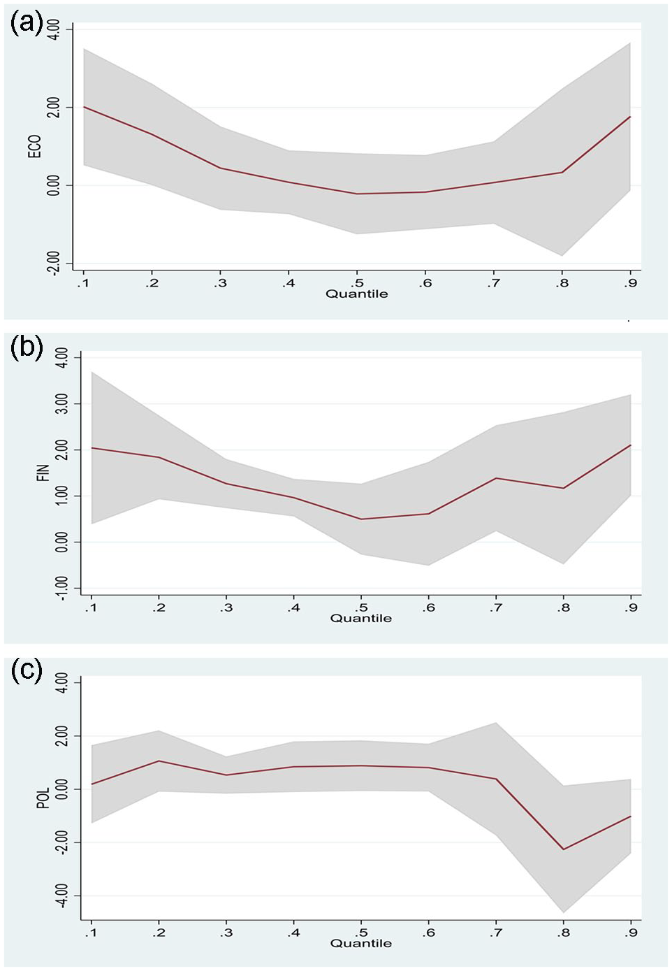
(a) The impacts of the economic risk rating score on international tourist arrivals. (b) The impacts of the financial risk rating score on international tourist arrivals. (c) The impacts of the political risk rating score on international tourist arrivals.
From a statistical perspective in Figure 1a (1b), the impact of ECO (FIN) is significant at the 10% level and positive at the majority of quantiles. To be specific, the ECO (FIN) coefficient initially decreases from 2.017 (2.044) at the 10% quantile to 0.727 (1.576) at the 25% quantile and then slowly increases to 1.77 (2.109) at the 90% quantile. The positive coefficient means that an increase in ECO and FIN will increase TA. The coefficient of POL is insignificant at higher quantiles levels of TA, but is significant at lower and intermediate levels (see Figure 1c). This result implies that the promotion of TA may increase country risk rating. The results indicate that the influences of CRs are nonlinear, as the OLS method might overlook the individual and distributional heterogeneities. Policy makers of countries with lower TA should be aware of the beneficial effects of CR on TA.
Regarding control variables, RP and GDP are positively and significantly related with TA, while FDI, EXG, and UMP are negatively related with TA. GDP positively influences TA, which is consistent with Saha and Yap (2014) in that governments of high-income countries can afford to invest funds to build up and maintain infrastructures for the tourism industry, which in turn attracts more tourists, expecting that a high income increases demand for tourism. However, the positive impact of RP is inconsistent with prior studies (Choong-Ki, Var, and Blaine 1996; Aki 1998). Muchapondwa and Pimhidzai (2011) present no significant relationship between relative prices and tourism demand, because the enhancement of the quality of services to tourists in order to reinforce taste formation is important for attracting more international tourists.
Using a destination country’s CPI as proxy of RP for the robustness test, we obtain a positive RP effect (we omit the CPI results to save space). Increases in tourism goods and service prices negatively affect tourism demand in a destination, as shown in many empirical studies (Hiemstra and Wong 2002; Garín-Muñoz and Montero-Martín 2007). However, a few other studies find no significant relationship between tourism goods and service price and tourism demand (e.g., Muchapondwa and Pimhidzai 2011). Tsai et al. (2006) pinpoint that “fluctuation in CPI may make tourists feel visiting and staying in Las Vegas a relatively more expensive or cheaper decision. Either a positive or a negative coefficient of CPI could be expected.” According to Arain et al. (2020) for France, Germany, Italy, the United Kingdom, and the United States, the most prominent relationship among tourism activities and FDI inflows are observed merely during the time of a deep economic recession; however, the negative nexus between tourism and FDI is noticed in some quantiles for China, Russia, Mexico, Spain, and Turkey, possibly because of the limited direct impact of tourism to these particular markets. We also find a negative relation between FDI and TA.
Our negative UMP effect is similar to Inchausti-Sintes (2015) who shows that tourism promotes economic growth and reduces unemployment. The negative EXG effect is in line with Hanafiah, Harun, and Jamaluddin (2011) in that tourism demand negatively correlates with the exchange rate. In addition, Forsyth, Dwyer, and Spurr (2014) find a higher exchange rate poses significant problems for tourism. Thus, the expected positive (negative) effects of GDP and RP (UMP, FDI, and EXG) are validated, whereas OIL and CRISIS do not show salient impacts. In sum, TA is sensitive to macro-economic variables.
Impacts of Country Risk Rating on International Tourism Revenues
Table 2 shows quantile estimates from equation (2). Figure 2 reports MMQR parameter estimates for the predictive power of CR effect on TR distribution for different TR components. Coefficient estimates are on the y-axis, while the quantile index is on the x-axis. The solid line shows the point estimation results at different quantile levels, and the shaded bands represent the corresponding 90% confidence intervals. Figures 2a, 2b, and 2c noticeably display that the effects of ECO, FIN, and POL on TR are individually diverse across different TR quantiles. The results in Table 2 also show that ECO (FIN) saliently and positively influences TR at the highest (lower and higher) TR quantile(s), partially supporting hypotheses H2a and H2b that ECO and FIN (country stability) have significantly positive effects on partial quantiles of TR. To be specific, the FIN coefficient initially increases from 1.237 at the 25% quantile to 1.292 at the 75% quantile and then saliently increases to 1.684 at the 90% quantile. The positive coefficient means that an increase in FIN will increase TR, suggesting that lower financial risk increases tourism revenues. However, we observe negative and significant impacts of POL at the highest quantile, signifying that the effects of CR are diverse across TR quantiles. In line with the results of TA, FIN is the most notable CR versus POL and ECO. Past related literature focuses on POL or a composite country risk, while our findings provide evidence that the multidimensional risk measure gives a more comprehensive evaluation. Additionally, the effects of CR are diverse across different TR quantiles.
Estimates of the MMQR-Based International Tourism Revenue Models.
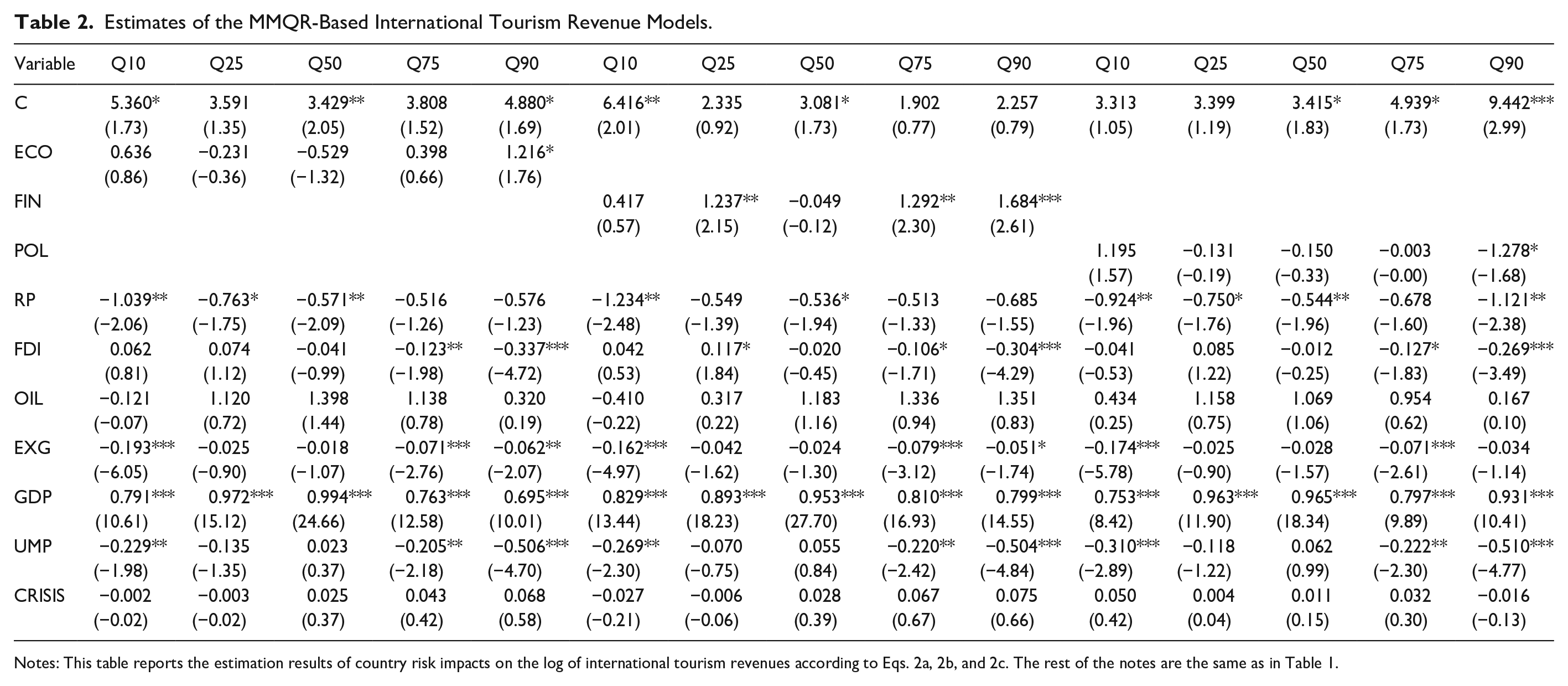
Notes: This table reports the estimation results of country risk impacts on the log of international tourism revenues according to Eqs. 2a, 2b, and 2c. The rest of the notes are the same as in Table 1.

a. The impacts of the economic risk rating score on international tourism revenues.
Regarding control variables, GDP (EXG, UMP, FDI, and RP) has a notably positive (negative) impact(s) on TR at some of the TR quantiles. Our finding is in line with Hiemstra and Wong (2002) and Garín-Muñoz and Montero-Martín (2007) whereby increases in tourism goods and service prices negatively affect tourism demand in a destination. GDP has a salient and positive impact on most of the TR quantiles, which is consistent with Ghalia et al. (2019) and Saha and Yap (2014) in that GDP per capita positively correlates with tourism flows. Martins, Gan, and Ferreira-Lopes (2017) pinpoint evidence that an increase in the World’s GDP per capita, a depreciation of the national currency, and a decline of relative domestic prices do help boost tourism demand. The negative UMP effect is similar to Inchausti-Sintes (2015) who note that tourism promotes economic growth and reduces unemployment. Like in Table 1, the TR result is also in line with Hanafiah, Harun, and Jamaluddin (2011) in that tourism demand negatively correlates with the exchange rate. Thus, the expected positive (negative) effect(s) of GDP (RP, UMP, and EXG) are validated, whereas FDI does not show any expected signs. In sum, the salient effects of macro-economic variables on TR are diverse across different TR quantiles. The positive effect of GDP on all TR quantiles suggests that increasing GDP leads to a greater TR. However, OIL and CRISIS do not show any salient effect on TR.
Impacts of Country Risk Rating on Travel and Leisure Sector Returns
Table 3 shows the estimates of the MMQR model introduced by equation (3). FIN has no significant impact on SR at all quantiles. The impact of ECO notably positively influences SR at the 10%–75% quantiles, revealing that ECO promotes tourism revenues, whereas the increasing effects tend to disappear at the highest SR quantile countries. POL has salient impacts on SR at the lowest and intermediate SR quantiles, revealing that POL is an important factor especially for countries at the lowest and intermediate SR quantiles. To be specific, the ECO coefficient initially increases from 1.238 at the 10% quantile to 1.778 at the 50% quantile and then saliently increases to 2.071 at the 75% quantile, revealing that lower economic risk denotes higher SR for countries with 10%–75% SR quantiles. The positive coefficient means that an increase in ECO and FIN will raise SR.
Estimates of the MMQR-Based Travel and Leisure Sector Return Models.
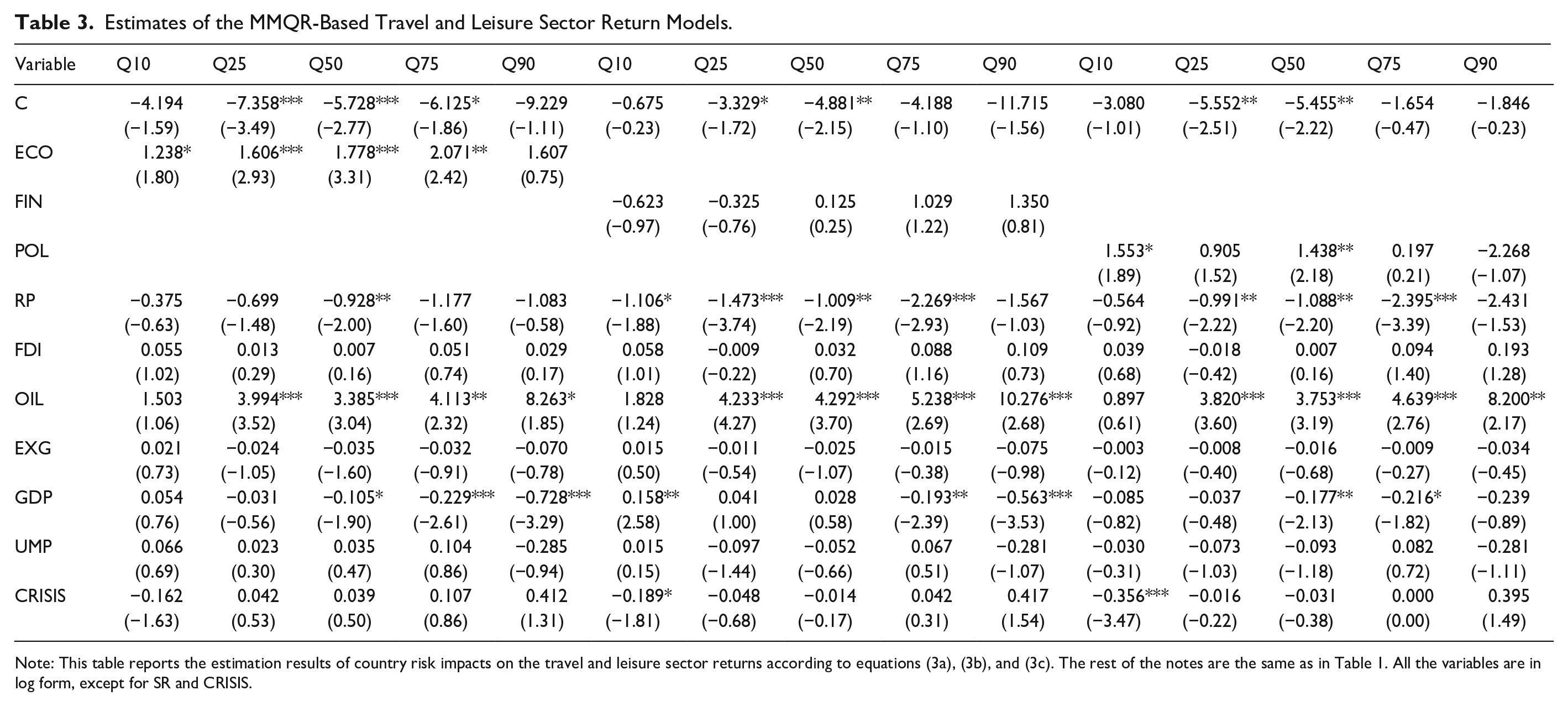
Note: This table reports the estimation results of country risk impacts on the travel and leisure sector returns according to equations (3a), (3b), and (3c). The rest of the notes are the same as in Table 1. All the variables are in log form, except for SR and CRISIS.
Our findings thus partially support hypotheses 3a and 3c that ECO and POL (country stability) have significant effects on travel and leisure sector returns. Specifically, the evidence supports that higher ECO leads to higher SR except for the highest SR quantile, and that POL only significantly affects the lowest and intermediate SR quantiles. Hence, the effects of ECO and POL are nonlinear. This is consistent with Liu, Hammoudeh, and Thompson (2013) whereby for all five members of BRICS, the relationships between the stock market and the three risk rating variables of each country respond asymmetrically to shocks. The results of SR that ECO, FIN, and POL have no significant effects on the highest SR quantile are in line with Muzindutsi and Manaliyo (2016) in that South Africa’s tourism revenues have continued to grow, even during the period of increasing political risk, and suggest further analysis is needed for how different dimensions of political risk affect different categories of tourism revenues.
The results for control variables included in the model are also informative. RP, GDP, and CRISIS show generally salient negative impacts on SR quantiles, while OIL shows notably positive impacts on SR. There is a sizable strand in the literature on the relationship between oil prices and stock prices, and their results are mixed (Bai and Koong 2018). Nonlinearities in the oil price–stock returns relationship occur, as stock returns respond to oil prices differently in periods of low and high economic volatilities associated with recessions or booms (Smyth and Narayan 2018). Mohaddes and Pesaran (2017) find no stable relationship between oil prices and stock returns in the United States over the period 1946-2017. Tsai (2015) shows that US stock returns responded differently to oil price shocks before, during, and after the global financial crisis. Interestingly, Apergis and Miller (2009) state that oil market shocks do not have a very large or significant impact on stock prices. Therefore, the impact of oil price on stock returns is not always negative. The negative RP impact on SR is consistent with Hiemstra and Wong (2002) as well as Garín-Muñoz and Montero-Martín (2007) in that increases in RP negatively affect tourism demand in a destination. The expected positive (negative) effects of OIL (RP and CRISIS) are validated. However, EXG and UMP do not show any salient effect on SR. In sum, the salient effects of macroeconomic variables on SR are nonlinear and diverse across different SR quantiles.
Our findings indicate that the ECO-SR nexus is generally remarkable, which is consistent with Ghalia et al. (2019), whereby institutional quality and absence of conflict are the driving factors that foster tourism flows for both source and destination countries. Our findings suggest that higher country risk ratings (i.e., better institutional environments/more stability) can boost SR for the nonhighest quantile SR countries where tourism development is needed. In the following robustness checks section, we further test the impact of the time-lag effect, different risk-level country, country development condition, and geographic area.
Table 4 displays the associated p values for the equality of quantile slope coefficients across the various pairs of quantiles. The tests confirm the visual inspection, revealing the F tests reject the null hypothesis of homogeneous coefficients at the 10% significance level for TA and TR pairs of quantiles and indicating that the impact of the explanatory variables is different across the different parts of the TA and TR distributions, except for the nexuses of CR-SR quantile level changes.
Statistic Tests of the Equality of Slope Estimates across Various Quantiles between Country Risk and Tourism Development.
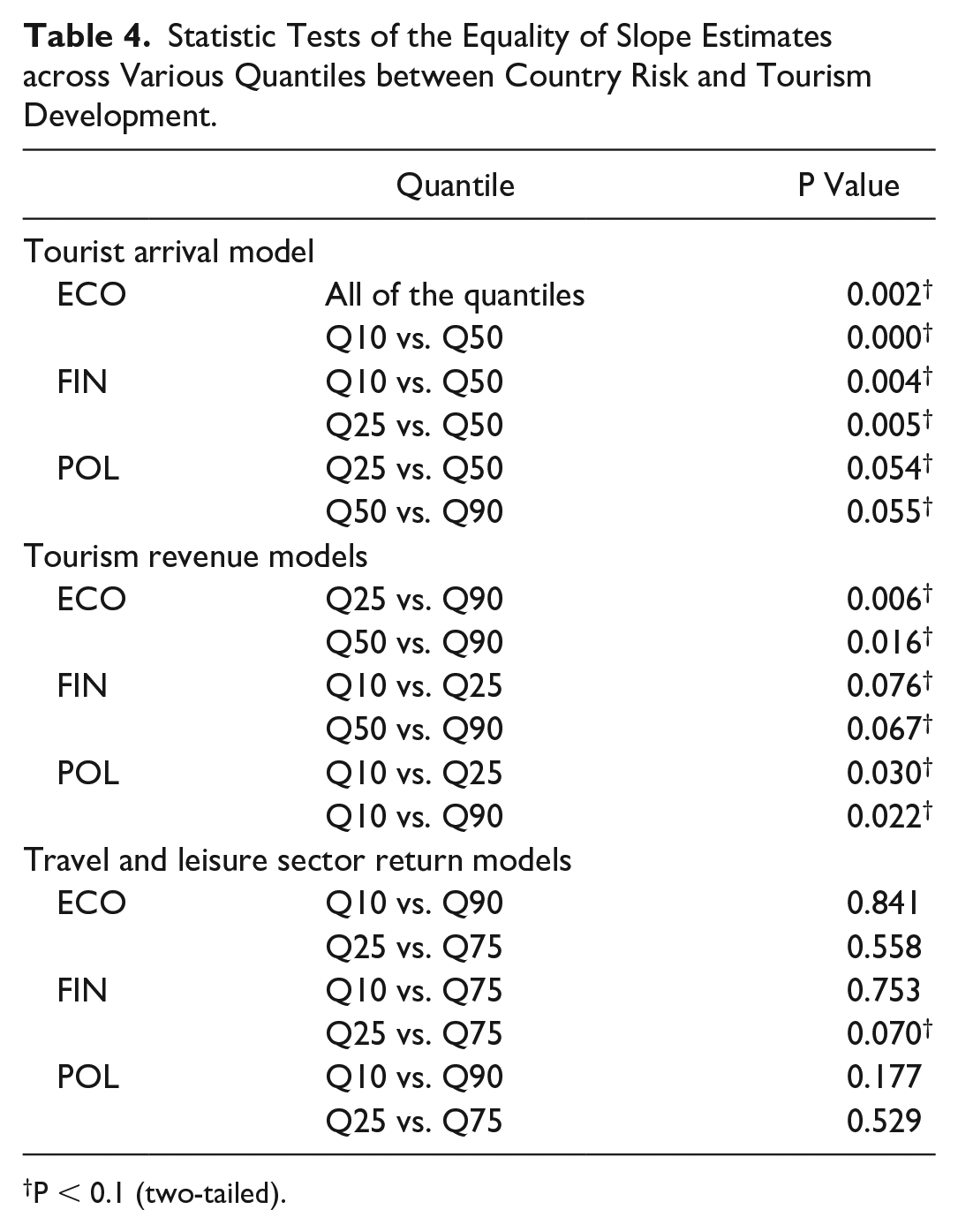
P < 0.1 (two-tailed).
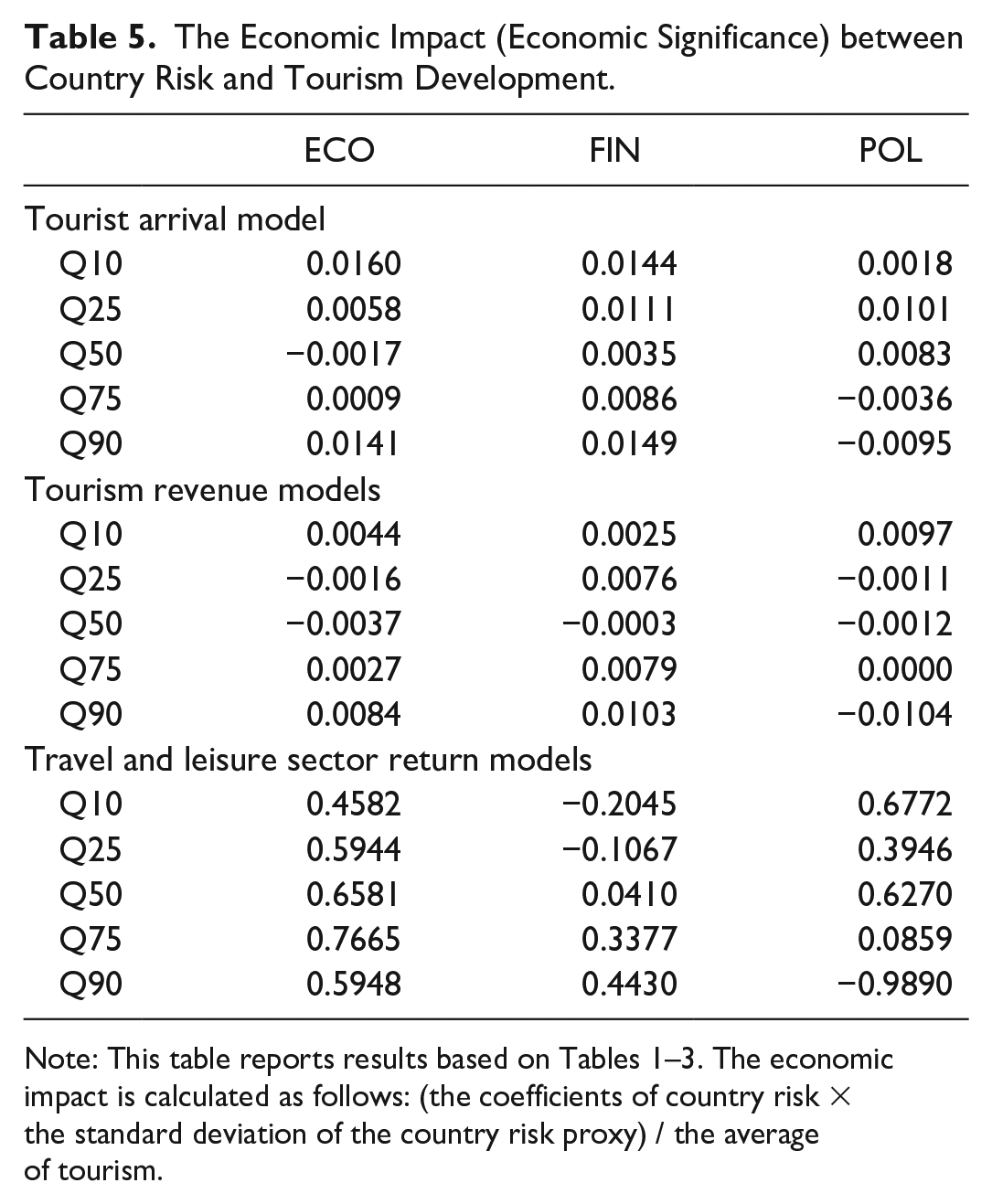
The economic impacts are shown in Table 5. We multiply the standard deviation of country risk and the coefficient of country on three risk proxies and divide by the mean of the three tourism proxies. For instance, we look at the economic impacts: the ECO coefficient (Q1) of 2.017 on TA implies that a one–standard deviation change of that economic risk rating on tourist arrivals is about 1.6%. As shown in Table 5, the economic impact of ECO is 0.58%, –0.17%, 0.09%, and 1.41% for the 25%, 50%, 75%, and 90% TA quantiles, respectively. We observe that the economic impacts of FIN (ECO) on TA (SR) all have a positive economic significance, implying that lower financial (economic) risk increases TA (SR). Comparably, the economic significances of ECO and POL are largest on SR among other nexuses, which is consistent with Erb, Harvey, and Viskanta (1996) that country risk ratings correlate with fundamental valuation attributes. However, there are some negative economic impacts for ECO on TA and TR, FIN on TR and SR, and POL on TA, TR, and SR. Thus, the economic impact of CRs on tourism development is nonlinear and asymmetric—that is, CRs improve tourism development (TD) at the majority of TD quantiles, while some are worse. However, we should note that Chen (2011) pinpoints that the movement of hotel stock price relies on not only a hotel firm’s current and future expected cash flows (measured by net income), but also on the perceived riskiness of stock cash flows from holding stocks (the discount rate). Thus, there exist other important variables to impact SR.
The Economic Impact (Economic Significance) between Country Risk and Tourism Development.
Robustness Checks
Effect of country risk rating on subsequent international tourism revenues
The results in Table 2 do not address issues regarding lag effect and/or endogeneity. To avoid this problem and incorporate the main variables into the models, in Table 6 we advance TR by one period to avoid simultaneity. This advance allows for the effect of any change in CRs to show up in TR. Comparing the CR impact of TR in Table 2 for concurrent as well as subsequent periods, the positive FIN-TR nexus (stability–tourism revenue) still holds for the higher and lower (25% and 75% as well as 90%) TR quantiles, indicating that FIN exerts a significantly positive and nonlinear impact on TR. However, POL shows a saliently positive impact on TR at the 10% quantile, but no significant impact of ECO on subsequent TR. Our findings illustrate that FIN has both concurrent and lagged effects on TR. In line with the results of TR, FIN is the most notable factor effect compared with POL and ECO. Additionally, different CRs exert diverse impacts on TR. Moreover, RP, EXG, FDI, and UMP (GDP) show saliently negative (positive) impacts on the subsequent TR. The findings of Tables 1–6 support hypothesis 4 in that the relationships between country risks and tourism development are nonlinear, varying at different quantiles of tourism distribution.
Estimates of the MMQR-Based International Tourism Revenues of Period t+1’s Models.
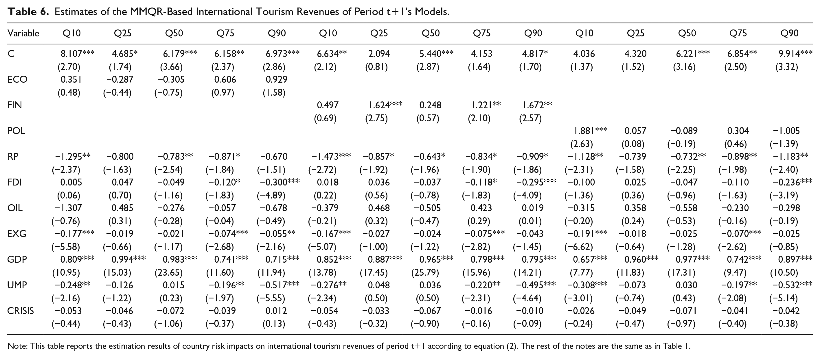
Note: This table reports the estimation results of country risk impacts on international tourism revenues of period t+1 according to equation (2). The rest of the notes are the same as in Table 1.
Comparisons of the results of high- and low-stability countries
To assess how different levels of CR affect TR, we replicate the analysis with subgroup samples by using the average of composite country risk ratings divided into high- and low-risk rating countries (i.e., high- and lower-stability countries), instead of the full sample. In this regard, Table 7 summarizes the results of the two subgroups. Evidence shows that regarding low-CR countries (instability countries), POL (FIN) has a positive impact on the intermediate (lower) and highest quantiles of TR, whereas ECO has no salient impact on TR quantiles. FIN (ECO) has a positive impact at the higher (highest) quantiles of stability countries, whereas POL has no salient impact on TR. This indicates that CRs exert diverse impacts between high and low risk rating countries. Thus, high-risk countries with higher TR can improve their ECO and FIN in order to increase TR. Low-risk courtiers can improve their FIN and POL to increase their TR. Our findings show the diverse impacts of CR on TR for high- and low-stability countries. Policy makers should know their countries’ tourism condition and then find the appropriate CR strategy to improve their TR.
Estimates of the MMQR-Based Comparison between High- and Low-Risk Impacts on Tourism Revenue.
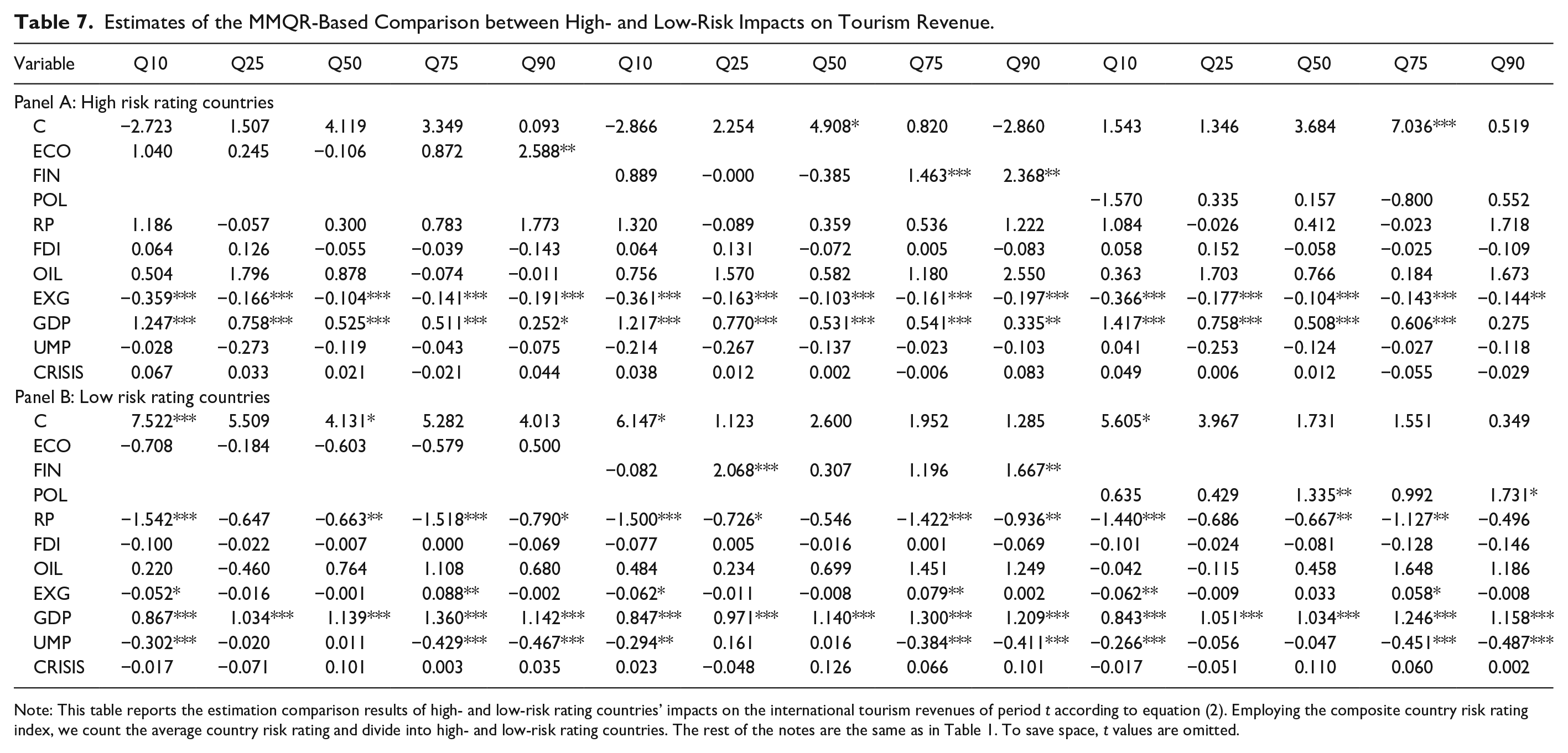
Note: This table reports the estimation comparison results of high- and low-risk rating countries’ impacts on the international tourism revenues of period t according to equation (2). Employing the composite country risk rating index, we count the average country risk rating and divide into high- and low-risk rating countries. The rest of the notes are the same as in Table 1. To save space, t values are omitted.
Subsample of developing countries
Diamonte, Liew, and Stevens (1996) find that political risks have a greater influence on expected market returns in emerging markets than in developed markets. Tourism policy makers of a country play an important role in developing regulations to ensure tourists’ security and stability through control over resource mobility (Williams 2004). However, Eilat and Einav (2004) present that political risk is important for both developed and developing countries. We investigate whether CRs have different impacts on tourism using developing countries as the subsample and report the empirical results in Table 8. FIN and POL show a constant, notably positive relation with TA and TR at several quantiles, suggesting that higher levels of FIN and POL (more stability) imply higher TA and TR for developing countries. However, the nexuses of ECO-TR and ECO-TA show no salient relations. As Shareef and Hoti (2005) state, the economies of developing countries, which have limited resources and need consistent inflow of foreign direct investment to maintain economic growth, are perceived to suffer from frequent disasters, and the international financial community considers them to be risky entities. Therefore, policy makers, tourism investors, and related participants of developing countries should be sensitive to FIN and POL country risks.
Estimates of the MMQR-Based International Tourist Arrivals and Tourism Revenues for Developing Countries.
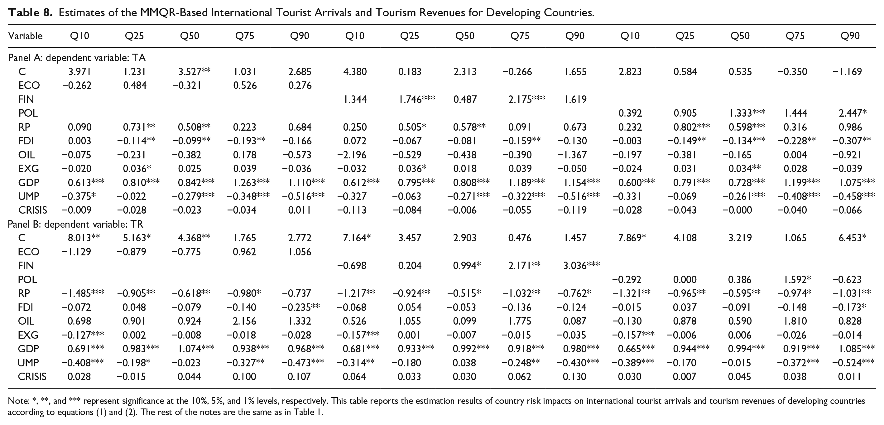
Note: *, **, and *** represent significance at the 10%, 5%, and 1% levels, respectively. This table reports the estimation results of country risk impacts on international tourist arrivals and tourism revenues of developing countries according to equations (1) and (2). The rest of the notes are the same as in Table 1.
Subsample of European countries
According to the website of International Tourism Highlights (2019) from the World Tourism Organization, Europe accounts for half of the world’s international arrivals and receives almost 40% of international tourism revenues, followed by Asia and the Pacific. Because the association between tourism revenue and GDP varies with geographic areas (Çağlayan, Sak, and Karymshakov 2012), we use the largest sample area, 33 European countries, as a subgroup to test the robustness of CR indices of specific region samples in Table 9. Regarding European countries, POL (ECO) shows significantly negative (positive) impacts on TA and TR. However, FIN shows an asymmetric impact on TR. Compared with the full sample, we find several differences in the results of the European countries.
Estimates of the MMQR-Based Tourist Arrivals and International Tourism Revenues of European Countries.
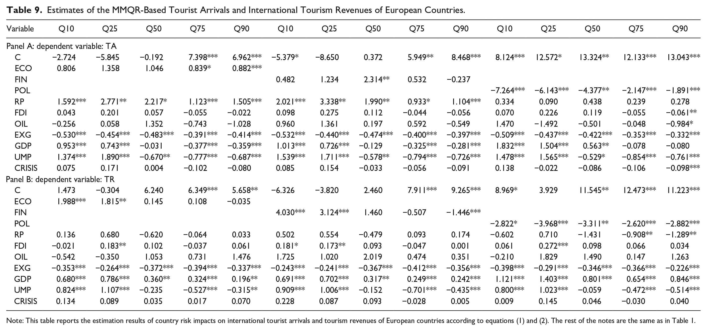
Note: This table reports the estimation results of country risk impacts on international tourist arrivals and tourism revenues of European countries according to equations (1) and (2). The rest of the notes are the same as in Table 1.
Alternative country crisis results
Following Laeven and Valencia (2020) and Lee and Lin (2018), we set different countries up with their own different financial crisis year (the delimitation crisis) dummy to test the robustness of CR indices in different crisis periods in Table 10. FIN (POL) shows significantly positive (negative) impacts on TR at all quantiles (at the highest quantile). The finding of a negative POL impact at the highest quantile is the same with Table 2 after using the global crisis (2008–2009) dummy, suggesting that nations with highest tourism revenues should account for the negative impact of political stability strategy. Therefore, the finding using the delimitation crisis year dummy supports our findings above. We summarize the findings in Table A6.
Estimates of the MMQR-Based International Tourism Revenue Models with Delimitation of Crisis Year.
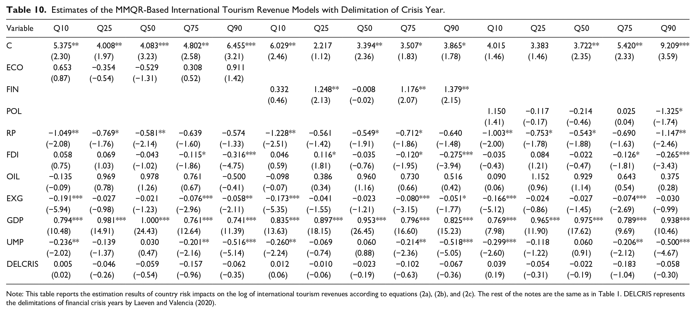
Note: This table reports the estimation results of country risk impacts on the log of international tourism revenues according to equations (2a), (2b), and (2c). The rest of the notes are the same as in Table 1. DELCRIS represents the delimitations of financial crisis years by Laeven and Valencia (2020).
Implications and Discussion
Our results in this study have several implications. First, our findings raise questions on whether it is prudent to use a composite country risk rating or merely a political risk rating as a single variable when studying country risks’ impacts on tourism development. Our findings show that different prospects of CRs diversely influence tourism development, and thus merely using a composite country risk rating or a political risk rating might not provide the full picture of CRs’ impact on tourism development. Second, the significant changes in country stability’s impact across different tourism development quantiles show that it is important to account for CRs’ influence at different quantiles of tourism development countries over time. Our findings from MMQR reveal that financial stability is positively significant for tourism revenues and tourist arrivals for higher and lower quantiles, while economic stability is positively significant from the lowest to higher sector return quantiles. This implies that the positive relationship between financial stability and tourism development is insignificant at intermediate quantiles of the conditional distribution of tourism revenues and tourist arrivals, while economic stability benefits all travel and leisure sector returns except for the highest quantile. This implies that financial stability may probably account for a relatively important degree of tourism development.
A visual inspection of Figures 1 and 2 shows that the MMQR estimates of different country risk ratings follow different dynamics. The estimate of the economic risk rating has its most salient influential positive coefficient at most of the SR quantiles except for the highest one; while that of financial stability has its most notable influential positive coefficient on TR quantiles. This denotes that countries can improve their economic (financial) stability in order to upgrade their travel and leisure sector returns (tourist arrivals). This is arguably especially true for the highest- and lower-quantiles tourism development countries, where tourism conditions might change quickly.
Third, it is noteworthy to point out from the panel-quantile regression results that a developing country, which is much more dependent on tourism to improve its economy, might enhance financial and political stabilities to develop their tourism sector, while political stability hinders European countries’ tourism development. Our finding addresses that the three country risk ratings have no salient impact on countries at the lowest and intermediate tourism revenue quantiles, as well as at the highest SR quantile. In addition, financial stability exhibits little effect on countries’ travel and leisure sector returns. We observe that political stability negatively influences tourism revenues at the highest quantile.
The fact that there are significant and positive impacts of country stability on tourism has important implications for policy makers that govern institutional substantiality in order to optimize their economy. From the managerial perspective, travel and leisure managers should consider establishing early warning and response mechanisms for economic and political country risk changes. Finally, we observe that different impacts exist for the features of geography and country risk level. This suggests that a useful policy implication can only be made once the empirical tests take into account the evidence of factors’ sensitivity, as is done in this study.
Conclusion
There is a growing perception that the world is a riskier place to live and travel, which could have serious implications for tourism (Fischhoff, Nightingdale, and Iannotta 2001). Thus, the concerns over safety and physical security within tourism warrant greater attention and research (Reisinger and Mavondo 2005), which could help at implementing sound institutional environments and assist policy makers in developing economies. This article takes a comprehensive view of the impacts from three types of country stability on three aspects of tourism development. Specifically, this research studies the relationships between destination country stability as well as tourism development by paying special attention to the distributions of international tourist arrivals, international tourism revenues, and travel and leisure sector returns using yearly data of 106 countries/regions for the period 2006–2017.
The main purpose of this study is to explore if international evidence exists regarding whether country stability positively influences tourism development across the conditional distortion of tourism factors. For this purpose, we employ a new panel quantile regression approach (i.e., the method of moment quantile regression proposed by Machado and Silva [2019]), which allows for the analysis of the different impacts of the exogenous variables across different quantiles of the conditional distribution of country risk ratings and which is useful for a more robust assessment of the empirical relationship. Additionally, we consider that the dependence relationships might change because of macroeconomic factors, a time lag effect, geographic region, country economic development level, and countries’ level of different risk rating score.
Our results generally support that country stability positively influences international tourist arrivals, tourism revenues, and travel and leisure sector returns, revealing that country stabilities do promote tourism development. Moreover, compared to POL, both FIN and ECO have more effects on countries with higher tourism quantiles, revealing that the impacts of CR are different within different CR components. Based on our findings, we support the hypothesis that country stability has significant positive impacts on tourism development, except for the hypothesis that political stability has a positive effect on international tourism revenues.
Our findings support that CR nonlinearly influences international tourist arrivals, international tourism revenues, and travel and leisure sector returns on different tourism development countries. Further test results reveal that the relationship mentioned above is robust when considering a time-lag effect, different risk-level countries, and country economic development conditions. There is a saliently negative significant effect of POL for the subsample of European countries. Moreover, political (economic) stability has little impact on high- (low-) risk rating subgroup countries, implying that geographic characteristics and country risk-level differences exist in the CR–tourism nexus. Generally, we find that the significantly negative unemployment, relative prices, exchange rate, and positive GDP effects are similar with prior studies, whereas the impacts of OIL and FDI are inconsistent. Overall, it means that tourism development is sensitive to the influences of macroeconomic factors.
Instead of focusing attention on political risk or the composite country risk rating as they relate to tourism, we broaden the scope of analysis by investigating the subcomponents of country risk (i.e., economic risk, financial risk, and political risk) on international tourist arrivals, international tourism revenues, and travel and leisure sector returns, so as to gain more comprehensive insights for international evidence in the related literature. As we focus the discussion on three country risk ratings, there are other country risk issues we have omitted, such as natural disaster risk, geopolitical risk, and infectious disease risk (e.g., COVID-19), which could enhance our understanding of the country risk effects on tourism. This is one limitation of this study. Additionally, the economic risk rating score consists of the following 5 subcomponents: Risk for per capita GDP, Risk for GDP growth, Risk for inflation, Risk for budget balance, and Risk for current account. The financial risk rating consists of the following 5 subcomponents: Risk for foreign debt, Risk for debt service, Risk for current account, Risk for international liquidity, and Risk for exchange rate stability. The political risk rating consists of the following 12 subcomponents: Government stability, Socioeconomic conditions, Investment profile, Internal conflict, External conflict, Corruption, Military in politics, Religious tensions, Law and order, Ethnic tensions, Democratic accountability, and Bureaucracy quality (ICRG). For further research, it would be interesting to examine the impact of these 22 components of CRs on tourism. Admittedly, we do not explore the relationship between such detailed country risk rating items and tourism, but it would be of great benefit to further explore the specific effects of every item and the distinct roles they may play in tourism development. We leave this work for the future.
Supplemental Material
Appendix – Supplemental material for Do Country Risks Matter for Tourism Development? International Evidence
Supplemental material, Appendix for Do Country Risks Matter for Tourism Development? International Evidence by Chien-Chiang Lee and Mei-Ping Chen in Journal of Travel Research
Footnotes
Acknowledgements
The authors are grateful to the insightful comments and suggestions from the Editor and two anonymous referees on the earlier draft of this paper. The help in preparation of the article from WenWu Xing (at School of Economics and Management of Nanchang University, China) is deeply acknowledged. Mei-Ping Chen gratefully acknowledges the financial support from the National Taichung University of Science & Technology, Taiwan. Chiang Lee gratefully acknowledges the financial support from Natural Science Foundation of Jiangxi Province of China (Grant No: 20202BAB201006). The authors declare no relevant or material financial interests that relate to the research described in this article.
Availability of data
Data are available from the authors upon request.
Declaration of Conflicting Interests
The author(s) declared no potential conflicts of interest with respect to the research, authorship, and/or publication of this article.
Funding
The author(s) disclosed receipt of the following financial support for the research, authorship, and/or publication of this article: Mei-Ping Chen is very grateful for financial support from National Taichung University of Science & Technology in Taiwan. Chien-Chiang Lee gratefully acknowledges the financial support from Natural Science Foundation of Jiangxi Province of China (Grant No: 20202BAB201006).
Supplemental Material
Supplemental material for this article is available online.
Author Biographies
References
Supplementary Material
Please find the following supplemental material available below.
For Open Access articles published under a Creative Commons License, all supplemental material carries the same license as the article it is associated with.
For non-Open Access articles published, all supplemental material carries a non-exclusive license, and permission requests for re-use of supplemental material or any part of supplemental material shall be sent directly to the copyright owner as specified in the copyright notice associated with the article.