






Abstract
Count responses with grouping and right censoring have long been used in surveys to study a variety of behaviors, status, and attitudes. Yet grouping or right-censoring decisions of count responses still rely on arbitrary choices made by researchers. We develop a new method for evaluating grouping and right-censoring decisions of count responses from a (semisupervised) machine-learning perspective. This article uses Poisson multinomial mixture models to conceptualize the data-generating process of count responses with grouping and right censoring and demonstrates the link between grouping-scheme choices and asymptotic distributions of the Poisson mixture. To search for the optimal grouping scheme maximizing objective functions of the Fisher information (matrix), an innovative three-step M algorithm is then proposed to process infinitely many grouping schemes based on Bayesian A-, D-, and E-optimalities. A new R package is developed to implement this algorithm and evaluate grouping schemes of count responses. Results show that an optimal grouping scheme not only leads to a more efficient sampling design but also outperforms a nonoptimal one even if the latter has more groups.
Keywords
The design of count responses in surveys is a common yet understudied topic in social sciences. Although the collection of exact counts of frequencies or incidence in social, epidemiological, and demographic surveys (e.g., number of births, frequencies of delinquent behaviors, incidents of diseases, and counts of social contacts) is analytically appealing, actual count responses in survey questions often consist of grouped counts (e.g., one response category “3–4 times” instead of two separate “3 times” and “4 times” categories) or are right-censored (e.g., the upper end response category as “6 or more times”). In fact, such grouped and right-censoring (GRC) count responses have long been adopted by social scientists to study a range of behaviors, events, and attitudes (Akers et al. 1989; Bachman, Johnston, and O’Malley 1990; Bailey, Flewelling, and Valley Rachal 1992; Barnes et al. 2006; Basu and Famoye 2004; Fu, Land, and Lamb 2013, 2016; Hagan, Shedd, and Payne 2005; Marsden 2003; Reardon and Raudenbush 2006; Schaeffer and Dykema 2011; Straus, Gelles, and Smith 1990; Thoits and Hewitt 2001). Scholars often find that GRC count responses are useful to study sensitive research topics (e.g., juvenile delinquency, domestic violence, and drug use) or to solicit information from respondents with less cognitive capacity (e.g., young adolescents or the oldest old). For example, one nationally representative survey project in the United States, the monitoring the future (MTF) study (or the National High School Senior Survey), has used GRC count responses to track annual trends of delinquency and substance use among U.S. high school seniors since the 1975. Such GRC count responses have also been used by the National Longitudinal Study of Adolescent Health (Add Health) to study adolescent behaviors at home, school, or neighborhood.
As documented in existing literature (Bradburn, Sudman, and Wansink 2004; Schwarz et al. 1985), the design of GRC count responses has a direct impact on the estimation of behavioral or cognitive frequencies. For example, an experimental study shows that the choice of right-censored count categories influences the estimation of TV-watching time Schwarz et al. (1985). Yet the design of GRC count responses is still arbitrarily determined by survey investigators. This practice is surprising, given the abundant presence of count responses with either right censoring or grouping or both in surveys. Under certain scenarios, determining the optimal grouping scheme of GRC count responses has been implemented by sophisticated statistical procedures and context-specific research designs, depending on the other variables of interest. For example, the intrinsic or contingent ordering of log-multiplicative association models may provide the optimal grouping scheme if conditional or joint distributions of variables in contingency tables are provided (Goodman 1987; Smith and Garnier 1986; Wong 2010). Likewise, given the extensive debates over the conceptualizations of gradations of democracy (Bollen 1990; Cheibub et al. 1996), it is found that the validity of dichotomous and graded measures of democracy can be evaluated by projecting their qualitative difference into two essential indicators related to democracy, international conflict, and regime stability (Elkins 2000). Although these innovative studies provide useful tools for scholars to assess grouping decisions for counts that are intrinsic to specific research questions at stake, their statistical procedures or research designs require additional information on the distribution of the ungrouped outcome variable and its association with other variables. Nevertheless, the use of GRC count responses often means that investigators have yet to understand the distribution of counts that are extrinsic to a specific research question, let alone its association with other variables. A search algorithm for the optimal grouping scheme focusing exclusively on the outcome variable per se rather than its research context is therefore useful and readily facilitates the evaluation of alternative grouping schemes with different a priori assumptions.
Applying the theory of optimal experimental designs (Atkinson, Donev, and Tobias 2007; De Leon and Atkinson 1991; Dette, Melas, and Pepelyshev 2004; Minkin 1987), we propose an innovative three-step algorithm for searching the parameter space and generating optimal grouping decisions for GRC count responses. In the machine-learning literature, optimal experimental design is also referred as a special case of semisupervised machine learning (or active learning) because a learning/search algorithm interacts with users (survey investigators for the current research) to obtain optimal outputs from the parameter space (Cohn, Ghahramani, and Jordan 1996; Settles 2010). Based on a Poisson multinomial mixture distribution, this article begins with configuring the data-generating process of GRC count responses and develops related maximum likelihood estimators. Two members of the Poisson family of frequency distributions, the Poisson and zeroinflated Poisson (ZIP), are studied in detail. Combined with prior Poisson distribution parameters, the Fisher information (matrix) of the maximum likelihood estimator is then employed to implement a new M search algorithm using Bayesian A-, D-, and E-optimalities. An R package [version 1.0]
GRC Count Data
Before discussing optimal designs for GRC count data, the question arises as to why such response categories have been adopted by social scientists. As examples, in various surveys, respondents are asked to list their numbers of close friends, weekly frequencies of alcohol intake, incidents of criminal victimization in the recent six months, times of illness in the last year, and lifetime history of residential moves. Admittedly, a precise enumeration of exact counts is methodologically appealing for two reasons. First, exact counts can be readily analyzed by existing statistical tools (e.g., Poisson regression models) and software packages. Second, survey investigators do not have to deal with arbitrary grouping or right-censoring decisions. Yet one major problem encountered by survey investigators is that the precise enumeration of counts can impose a cognitive burden on interviewees and sometimes leads to excessive missing data. In other words, the GRC data structure is a compromise between what survey investigators want and what respondents are willing or able to offer (Groves et al. 2011; Schaeffer and Presser 2003). For example, although medical sociologists and psychiatrists would like to know exactly how many days in the past week respondents experienced a variety of depressive symptoms, respondents, especially these with depressive symptoms, often get frustrated when required to distinguish between, for example, two days and three days. Thus, the Center for Epidemiological Studies-Depression (CES-D) scale, an established self-report depression measure, offers four grouped response categories: less than one day, one to two days, three to four days, and five to seven days (Radloff 1977). For a study on elder adults aged 65 and above, a pretest showed that respondents were unwilling to answer even the four grouped response categories of the CES-D scale, so researchers had to further collapse the four grouped categories and used a dichotomous measure instead (Blazer et al. 1991).
Likewise, for research topics that are perceived as sensitive or less socially desirable, such as personal income, number of sex partners, incidents of delinquent behaviors, and history of drug use, respondents feel more comfortable in reporting grouped or right-censored categories instead of exact numbers (Sudman, Bradburn, and Schwarz 1996). It is not surprising that most, if not all, questions related to the frequency of juvenile delinquency and drug use in both the MTF study and the Add Health adopted GRC count responses.
Even if respondents are willing to collaborate, the difficulty in recalling the exact number of events that happened some time (e.g., several months) ago makes the exact number of events unreliable and introduces additional measurement errors (Groves et al. 2011; Schaeffer and Presser 2003). Similarly, if listing the total number of events requires extra efforts during field interview, fatigue of interviewers can result in underreported numbers of events. For example, as interviewers were instructed to probe for more discussion partners, it has been shown that interviewer effects (e.g., the failure to elicit more private network data) contributed to the extensive debates concerning increasing social isolation in the United States (Paik and Sanchagrin 2013).
Generating GRC Count Data
In order to define the optimality for objective functions of GRC grouping schemes, we first configure a data-generating process for GRC count responses. The Poisson distribution is often used to model count data with probability mass:
where y is a random count variable and λ is both the mean and the variance of the Poisson distribution. To define a Poisson-based likelihood function for GRC count data, we propose a data-generating scheme in the form of a Poisson multinomial process. Similar Poisson multinomial models were previously used to study contingency tables and traffic accidents (Lang 2004; Lord, Washington, and Ivan 2005).
We let
In other words, we have a N-dimensional random vector
For example, the multinomial distribution corresponding to
The probability mass function of
If there are n independent observations
Because this likelihood function derives from a Poisson multinomial distribution, it is easy to show that the corresponding maximum likelihood estimator is consistent and asymptotically normal. More importantly, the variance of its asymptotic distribution is given by the inverse of the Fisher information.
1
In other words, any consistent sequence
The Poisson distribution assumes that its mean λ equals variance. However, this assumption is violated if empirical frequency distributions show excess zeros relative to a Poisson distribution (Hall 2000; Klein, Kneib, and Lang 2015; Lambert 1992; Puig and Valero 2006). The ZIP distribution takes excess zeros into account and has the probability mass function:
where p is the proportion of population exposed to the
Using the same distribution of α
j
in equation (2), the GRC data
The probability mass function of α then depends on two parameters p and λ of the ZIP distribution,
Again, based on Theorem 6.5.1 at Lehmann and Casella (1998), it is easy to show that the maximum likelihood estimators remain consistent and asymptotically normal for the ZIP case. The detailed proof of their asymptotic properties is given in Fu, Guo, and Land (2018). Estimators
where J11 and J22 are the 1-1 and 2-2 entry of the Fisher information matrix
Optimal Designs for GRC Count Data
The foregoing demonstration that the asymptotic distributions of the maximum likelihood estimators of both the Poisson and the ZIP cases are characterized by the Fisher information (matrix) is important for defining Bayesian optimality of GRC grouping schemes, given the internal link between Fisher information (matrix) and grouping choices. For example, the Fisher information of the Poisson case depends on both the true unknown parameter λ0 and the specific grouping scheme G: If we know the true parameter λ0, the corresponding asymptotic distribution of the estimator
Fisher Information and Grouping Choices: the Poisson Case
For the Poisson case, the Fisher information of the previous Poisson multinomial distribution with parameter λ and the grouping scheme
Equation (7) follows the definition of probability mass function θ
j
in equation (3) and
where
In inequality (8), we note that the equality holds if and only if
Likewise, for special cases where
Given that a < b < c, the coefficients of the polynomial
We previously noted that the Fisher information of the Poisson case depends on both the specific grouping scheme G and the true (unknown) parameter λ. Given the foregoing three remarks on the relationship between grouping choices and Fisher information, a probability function ρ can be defined to take prior knowledge of λ into account. In general, we define an objective function as
where ρ is a continuous or discrete distribution. The introduction of ρ allows analysts to deal with the uncertainty in estimating the true parameter λ and explore optimal grouping schemes under different prior distributions. For example, if a survey investigator assumes that the true value of λ is known, ρ becomes a degenerate distribution with a point mass of 1 at
ρ can also be specified as a discrete distribution supported on positive numbers
Fisher Information and Grouping Choices: The ZIP Case
Given that the ZIP distribution has two parameters p and λ, its corresponding Fisher information is denoted by a symmetric and positive semidefinite matrix:
where
where
The Fisher information matrix
For both the Poisson and the ZIP cases, we have demonstrated that asymptotic variances are given by the inverse of Fisher information (matrix). Given that in experimental designs an optimal design is often selected to yield the most efficient estimator (see, e.g., Steinberg and Hunter 1984), an optimal grouping scheme of GRC data should, according to the same principle, maximize Fisher information (matrices) and produce more (asymptotically) efficient estimators. Because there are multiple ways of ordering square matrices, we introduce a local objective function S to compare Fisher information matrices: Optimising S will give a locally optimal design (Chernoff 1953), where local means that the design is optimal for a specific value of an unknown parameter (or vector). To illustrate the definition of S, we follow previous research on the Loewner partial order (see, e.g., Horn and Johnson 2013) and write
To maximize the Fisher information matrix and achieve more efficient estimation, we apply local objective functions based on three common optimality criteria (Horn and Johnson 2013; Steinberg and Hunter 1984): A-optimality: maximizing
This conclusion that
Because both
If G* is obtained by dividing the first group of G into two subgroups, we have
Since
We use a distribution
Here, we choose to optimize the integral of
When
A Three-step M Algorithm
Considering a global objective function Ω(⋅) that is either ΩP or ΩZIP in the preceding section, we propose a three-step M search algorithm for selecting an optimal grouping scheme that maximizes Ω. It should be noted that the application of this algorithm is not restricted to GRC data but could be extended to optimal designs for count responses in general if either grouping or censoring is present. From the perspective of semisupervised machine learning, this M algorithm searches all possible combinations of grouping schemes and interacts with survey investigators to yield the optimal grouping scheme.
Remarks 4.3 and 4.6 show that a finer grouping scheme increases the value of Ω. Without grouping or right censoring, Ω is thus maximized by the finest scheme where each separate response group contains and only contains one integer. This finest possible grouping scheme is obviously the optimal one. In the presence of grouping and right censoring, however, the search for an optimal grouping scheme is constrained by the total number of groups N allowed. Now, the search becomes challenging, if not impossible, since the search algorithm has to deal with infinitely many grouping schemes. To make sure that the infinitely many grouping schemes for the GRC count responses can be processed by our search algorithm, we introduce a hypothetical integer M, which is sufficiently large, to divide the infinitely many grouping schemes into two parts: a finite set where M is contained in the last groups of schemes and an infinite set where M is not contained in the last groups. With the introduction of M, the search algorithm consists of three major steps. First, we use M to produce a finite set of possible grouping schemes. An optimal grouping scheme maximizing Ω(⋅) is identified after a search of this finite set. The second and third steps verify whether the optimal grouping scheme returned by the first step is the global maximizer, that is, the scheme achieving the best performance among all N-group schemes. The search algorithm stops if the optimal grouping scheme returned by the first step passes the verification. Otherwise, the iteration continues with a larger M.
The introduction of M divides the whole set of infinite grouping schemes into two parts: a finite set with M contained in the last group and an infinite set with M not contained in the last group. This procedure is motivated by the idea that, if M is sufficiently large, all integers larger than M from a Poisson process cannot exert much influence on the Fisher information and thus do not affect the choice of optimal grouping schemes. To illustrate this idea, we define the last right-censored group IN of a N-group scheme
Moreover, an implication of this property is that, to increase the Fisher information, finer grouping decisions should be applied to integers with nontrivial probabilities. If the total number of groups N is fixed, a finer grouping of large integers with trivial probabilities should be avoided, and a coarse right-censored group is preferred.
The choice of M follows a Goldilocks rule. An important assumption of the search algorithm is that M should be sufficiently large and represents the lower bound of a set of integers leading to a successful search for the global optimal scheme. Yet researchers should not choose a too large M either: The number of all possible grouping schemes processed by the search algorithm grows quickly with larger M, and the search takes much longer time despite optimization of the algorithm (the computation time is roughly proportional to MN − 1). In theory, M should be the lowest integer included in the last right-censored group of the global optimal scheme, so that the search algorithm works without consuming too much time. As a practical guidance, researchers may start from an integer larger than the mean of the prior distribution of λ, gradually increase M if its previous value fails the verification from step 2 and 3, and locate a sufficiently large M in a trial and error learning process.
One example of the search algorithm is demonstrated in Figure 1. If we set N = 3 and M = 4, step 1 only searches six schemes as plotted in the part A of Figure 1. When M is not contained in the last group, there are infinitely many grouping schemes to search and their overall set is denoted as F1. Examples of F1 are plotted in the part B of Figure 1.
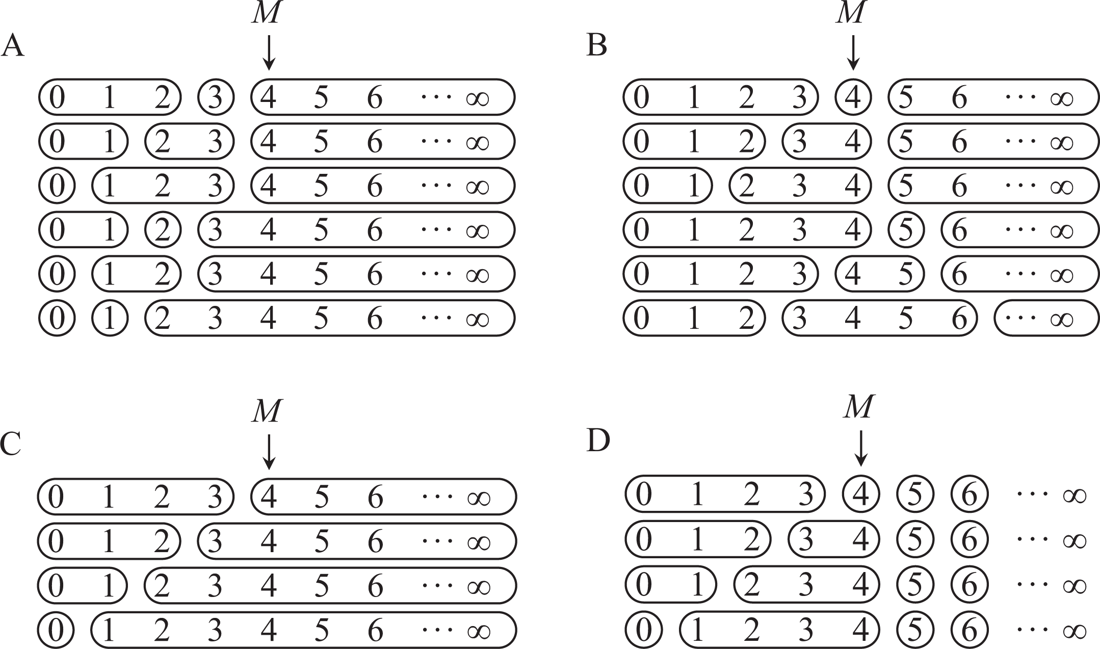
An illustration of the search algorithm. Part A: all possible three-group schemes with M = 4, where M is contained in their last groups; Part B: examples of infinitely many three-group schemes from the set F1, where M is not contained in their last groups; Part C: the set F2 of two-group schemes obtained from a merging process of schemes in part B. M is still contained in their last groups; Part D: the set F3 obtained from F2 by including each integer greater than M in one and only in one group.
The foregoing discussion in step 1 shows that our algorithm divides the set of all possible grouping schemes into two parts, and step 1 deals with the finite set with M contained in the last group. Step 2 then deals with the other infinite set F1 with M not contained in the last group. In step 2, the algorithm will search a finite set F3 of grouping schemes and calculate the objective function based on an optimal scheme from F3. To understand the second step, we first illustrate what F2 and F3 are and then discuss the relation between F1 and F3. First, let F2 be the overall set of (N − 1)-group schemes such that M is contained in the last group. When N = 3 and M = 4, F2 only consists of four schemes and is illustrated in the part C in Figure 1. Second, for each grouping scheme G in F2, we divide its tail after M to make a new scheme G′. Now, the first N − 2 groups in G′ are exactly the same as these in the corresponding G, but each integer greater than M is now contained and only contained in a separate group in G′. We denote F3 as the total set of all grouping schemes G′ obtained in this way from F2. The case with N = 3 and M = 4 is shown in parts C (for F2) and D (for F3) in Figure 1. Due to the one-to-one match between grouping schemes from F2 and F3, they have the same number of schemes.
For any N-group scheme G from F1, where M is not contained in the last group, F3 contains at least one scheme G′ finer than G. More specifically, if M is contained in the (N − 1)th group for a grouping scheme G, there exists some G′ in F3 that has identical first N − 2 groups as G. G′ must be finer than G, given that every integer beyond M is also contained in a separate group in G′. The case where M is contained in the kth group with k ≤ N − 2 can be deduced by analogy, as now the first N − 2 groups of G′ are finer than the first k − 1 groups of G.
The relationship among F1, F2, and F3 can be further conceptualized as follows. When M is not contained in the last group (as shown in F1), the search algorithm actually merges the group containing M with all its right side groups (including the right-censored group) to form a new and bigger right-censored group. The first three grouping schemes from part B to part C in Figure 1 illustrate this merging process. Subsequently, the new grouping scheme with a bigger right-censored group (e.g., the first scheme in part C) has fewer total number of groups and is thus coarser than its original form in F1 (e.g., the first scheme in part B). To make a fair comparison between Fisher information of grouping schemes with M contained in the last group and with M not contained in the last group, after the merging, we must compensate for the loss in the latter’s Fisher information due to this reduction in the total number of groups. To compensate for the loss of the Fisher information after merging, each integer greater than M in the new last group is subsequently contained and only contained in a separate group. This procedure thus forms a new (much) finer grouping scheme (i.e., from grouping schemes in part C to corresponding grouping schemes in part D). Step 3 then compares values of the objective functions between the optimal grouping scheme with M contained in the last group and the (much finer) optimal grouping scheme with M contained in other groups. Pseudocode describing the search algorithm is listed as below to facilitate readers’ understanding: Input the (maximum) number of groups N, a sufficiently large integer M and the objective function of a grouping scheme Ω; Among all N-group grouping schemes where M is contained in their last groups, find the scheme Gmax that maximizes Ω and denote this maximum value as Set F2 as the overall set of (N − 1)-group schemes where M is contained in the last group for every grouping scheme G in F2; For every G in F2, there exists one corresponding grouping scheme G′ where every integer greater than M is contained and only contained in one separate group. The total set of all such grouping schemes G′ is defined as F3. Find the grouping scheme in F3 that maximizes Ω and denote this maximum value as Ω*; Return Gmax if
To summarize, because there are infinitely many grouping schemes with M not contained in the last group (e.g., grouping schemes from the set F1 as shown in part B), we first transform them into finite schemes with M contained in a new (big) last group (F2 as shown in part C) and then much finer schemes (F3 as shown in part D) to do a fair comparison. It is clear that these much finer grouping schemes may sometimes overcompensate for loss in Fisher information in the merging process. For example, step 3 could falsely reject the true optimal grouping scheme if the M chosen is at or slightly higher than the lowest integer included in the last right-censored group of the global optimal scheme. Yet the false rejection can be easily solved by increasing the value of M as each separate group containing one integer larger than M plays less role in estimating the objective function. The global optimal grouping scheme successfully accepted by the algorithm remains the same as that falsely rejected. Actually, the search algorithm is intentionally developed in a way that it prevents any false acceptance of a wrong optimal scheme at the cost of tolerating false rejection of the true optimal grouping scheme, while a larger M further solves the false-rejection issue.
Data Simulation and Empirical Analysis
To illustrate the optimal designs for count data, we employ data from a nationally representative survey of youth in America, the MTF study. Since 1975, each year about 250,000 high school students from approximately 130 U.S. high schools nationwide participate in this survey. In the current study, we focus on four questions from the MTF study related to 12th graders’ frequencies of alcohol drinking from 1996 to 2012. The first three questions on alcohol drinking are virtually the same except for the reference period (in your lifetime, during the last 12 months, and during the last 30 days): “On how many occasions have you had alcoholic beverages to drink–more than just a few sips?” The GRC count response categories for the three questions are: 0 occasions, 1–2 occasions, 3–5 occasions, 6–9 occasions, 10–19 occasions, 20–39 occasions, and 40 or more. The fourth question is related to binge drinking: “Think back over the LAST TWO WEEKS. How many times have you had five or more drinks in a row? (A “drink” is a glass of wine, a bottle of beer, a wine cooler, a shot glass of liquor, a mixed drink, etc.).” GRC count response categories for this question are none, once, twice, 3–5 times, 6–9 times, and 10 or more times. Table 1 shows the original counts of drinking data from 1996 to 2012. Drinking behaviors tend to be less often with shorter reference periods. Binge drinking is most rare among the 12th graders.
Frequency Distributions of Adolescent Alcoholic Drinking, MTF, 1996–2012.

Note: MTF = monitoring the future.
To identify appropriate prior distributions for Bayesian optimal designs, we wrote an R function
Maximum Likelihood Estimates of Means and Standard Deviations (SD) of (Zero-inflated) Poisson Parameters.

Note: ZIP = zero-inflated Poisson.
Next, based on the aforementioned search algorithm, we developed another R function
N defines the (maximum) number of groups, which should be greater than one for the Poisson case and greater than two for the ZIP case. densityFUN gives the probability density function of a prior distribution, if needed. [
Estimated Optimal Grouping Schemes With Different Numbers of Groups: Uniform Prior Distributions.

Note: ZIP = zero-inflated Poisson.
aThe lowest M needed to find the global optimal grouping scheme.
Estimated Optimal Grouping Schemes With Different Numbers of Groups: Normal Prior Distributions.

Note: ZIP = zero-inflated Poisson.
aThe lowest M needed to find the global optimal grouping scheme.
Estimated Optimal Grouping Schemes With Different Numbers of Groups: Uniform Prior Distributions.

aThe lowest M needed to find the global optimal grouping scheme.
Based on results calculated by
which yields the same optimal grouping scheme as
We use a uniform distribution as the prior distribution in Table 3. It should be noted, however, that other continuous or discrete distributions can also be processed by the R function as the prior distribution. The third cell [0, 1, 2, 3-4, 5+] under the drinking in 30 days (Poisson) scenario means that the optimal grouping scheme is zero, once, twice, three and four times, and five times and more, given that the total number of groups is five and the range for λ’s prior distribution is [1.34, 4.02]. Across different scenarios, the lowest M required to identify the global optimal scheme is also provided. As the search algorithm tolerates false rejection, the lowest M is often slightly larger than the lowest integer of the last right-censored group of the optimal scheme, and this difference becomes larger as λ increases. Across the eight scenarios in Table 3, the cutoff integers between two adjacent groups tend to concentrate on smaller integers if the parameter space of λ is close to zero (the binge drinking scenario). If the parameter space of λ stays close to zero (e.g., rare events), any grouping decision of small integers is not supported by the search algorithm as the maximum number of groups N increases (see N = 7 or 8 in the binge drinking scenario). This finding suggests that the GRC count response is inappropriate for collecting very rare count events. The cutoff integers tend to appear first around the mean of the parameter space of λ and then appear at other locations as N increases. The prior distributions in Table 6 are truncated (mean ± 3 standard deviations) Gaussian distributions whose means and standard deviations are provided in Table 2. Table 4 also demonstrates that the cutoff integers of grouping decisions often exist at integers around which λ has higher probability density. For the same combination of N and range of prior distributions, the optimal schemes listed in Tables 3 and 4 are virtually the same, suggesting that the search for optimal schemes is not sensitive to the choice of prior distributions. Table 5 lists optimal grouping schemes when λ is low, moderate, high, and unspecified for readers’ reference. Because zero is contained in a separate group for the ZIP case from Tables 3–5, the optimal grouping scheme remains the same when λ is fixed but p varies.
Parameter Estimates for Different Grouping Schemes: Results From Simulation.

aEach simulation is repeated 1,000 times to calculate estimates. Numbers in the parentheses are sample sizes used for simulation.
bOptimal grouping schemes with fewer groups.
To illustrate how an optimal grouping scheme is preferred to other grouping schemes, we use the grouping scheme adopted by the MTF binge drinking question as a reference grouping scheme and compare standard errors estimated under different grouping schemes. In Table 6, the first column is the true parameters we used to simulate the Poisson distributions. Both parameters inferred from the data (see Table 2) and hypothetical parameters are used. The reference schemes are those adopted by the MTF study to measure alcohol drinking. The optimal schemes are generated by
When λ is small, the reference schemes appear to be acceptable as their corresponding standard errors are only slightly larger than these calculated based on optimal grouping schemes. However, the differences between standard errors estimated from the reference schemes and those of the optimal schemes grow larger as λ increases. As expected, the standard errors decrease by 10 when sample sizes increase by 10. Moreover, the strength of this algorithm can be illustrated by optimal schemes with fewer groups than corresponding reference schemes. Compared with estimation based on the reference schemes, researchers could achieve almost the same, sometimes better, efficiency of estimation by adopting optimal schemes with even smaller numbers of groups N. In other words, an optimal grouping scheme can outperform a nonoptimal one even if the latter has more groups.
Discussion and Conclusion
This research applies optimal experimental design, a branch of semisupervised machine learning, to social science research and provides a novel algorithm to find the optimal grouping scheme of GRC count responses. One of the most striking features of social science research on survey methodology is the degree to which the design of response categories in survey questions has been neglected. Count responses with grouping and right censoring have long been collected by social scientists to study a variety of behaviors, status, and attitudes. Yet there has been little research on optimal designs for discrete response categories such that grouping or right-censoring decisions often rely on arbitrary choices of survey investigators. To search for optimal grouping schemes, this article first uses Poisson multinomial mixture models to conceptualize the data-generating process of count data with grouping and right censoring and then investigates the relationship between grouping-scheme choices and asymptotic distributions of the Poisson multinomial models. Using different types of optimalities in experimental designs (De Leon and Atkinson 1991), we investigate local objective functions of the Fisher information (matrix) and further demonstrate the possibility of optimal designs for GRC count responses: The optimal grouping scheme should maximize the global objective function of the Fisher information (matrix). We also propose a new three-step general algorithm to process infinitely many grouping schemes and identify the global optimal grouping scheme. To process all possible grouping schemes, this algorithm introduces a sufficiently large integer M, which is in theory the lowest integer contained in the right-censored group of the global optimal scheme. The introduction of M not only makes the search feasible but also tolerates false rejection of the global optimal grouping scheme. A new R package
The M algorithm and software programs presented in this research readily provide survey investigators a new tool for evaluating grouping and right-censoring decisions of count responses in surveys. While survey methodologists do need to take a series of factors (e.g., the coherence of response categories over time and across questions or whether a specific count is of research interest or has substantive meaning) into account when designing response categories (Schaeffer and Dykema 2011), the new R package developed allow scholars to incorporate their prior knowledge in optimal designs of survey questions. Although this research only addresses (ZI) Poisson models of count data, it should be noted that the application of the M search algorithm is not restricted to the two statistical models investigated and can be extended to other models of count data such as negative binomial models and hurdle models. If the assumption that the Fisher information increases with a finer grouping scheme holds for other discrete or continuous data-generating processes, this M algorithm can be employed for designing survey responses in general. Such potential applications of this algorithm to broader issues in survey methodology merit further attention.
Footnotes
Acknowledgment
The authors would like to thank Junhui Wang, Jiahua Chen, Sayan Mukherjee, Li Ma, Ding-Xuan Zhou, Tim Liao, Zheng Wu, Nan Lin, Linda K. George, Yanlong Zhang, Yandong Zhao, and seminar/conference participants at University of Victoria, Shanghai University, the 2013 Joint Statistical Meetings (Montreal, Canada), and the 2015 Methodology Section Mid-year Meeting of American Sociological Association (San Diego, USA) for their helpful comments.
Declaration of Conflicting Interests
The author(s) declared no potential conflicts of interest with respect to the research, authorship, and/or publication of this article.
Funding
The author(s) disclosed receipt of the following financial support for the research, authorship, and/or publication of this article: The authors gratefully acknowledge the financial support from the Research Grants Council of Hong Kong (ECS Project No. PolyU 25301115), Hampton New Faculty Award at The University of British Columbia, Chiang Ching-kuo Foundation for International Scholarly Exchange and a 2015 Major Project of the National Social Sciences Foundation in China (grant no. 15ZDB172).