
Abstract
Analysts of discrete data often face the challenge of managing the tendency of inflation on certain values. When treated improperly, such phenomenon may lead to biased estimates and incorrect inferences. This study extends the existing literature on single-value inflated models and develops a general framework to handle variables with more than one inflated value. To assess the performance of the proposed maximum likelihood estimator, we conducted Monte Carlo experiments under several scenarios for different levels of inflated probabilities under multinomial, ordinal, Poisson, and zero-truncated Poisson outcomes with covariates. We found that ignoring the inflations leads to substantial bias and poor inference of the inflations—not only for the intercept(s) of the inflated categories but other coefficients as well. Specifically, higher values of inflated probabilities are associated with larger biases. By contrast, the generalized inflated discrete models (GIDMs) perform well with unbiased estimates and satisfactory coverages even when the number of parameters that need to be estimated is quite large. We showed that model fit criteria, such as Akaike information criterion, could be used in selecting the appropriate specifications of inflated models. Lastly, the GIDM was implemented using large-scale health survey data as a comparison to conventional modeling approaches such as various Poisson and Ordered Logit models. We showed that the GIDM fits the data better in general. The current work provides a practical approach to analyze multimodal data that exists in many fields, such as heaping in self-reported behavioral outcomes, inflated categories of indifference and neutral in attitude surveys, large amounts of zero, and low occurrences of delinquent behaviors.
Keywords
Introduction
Many of the quantitative variables used in social science studies are discrete in nature. Respondents typically choose from a limited number of categories on ordinal scales, and researchers have long recognized that such data have the tendency to include inflated values. Data inflation may take various forms. It could be that respondents forget the information, or round to a nearby number of convenience (Crawford, Weiss, and Suchard 2015); it can also be the result of hiding one’s ignorance in situations where face-saving is deemed important (Bagozzi and Mukherjee 2012). In other scenarios, measures on counts or summarized items, for example, the number of hospital visits and the delinquency scale, may naturally concentrate on values of zero or low occurrences such as one or two.
Depending on the assumptions about how the inflation was generated, two common modeling strategies are available to address the inflation on one value. The first strategy assumes the inflation is a form of data reporting error, referred to as “heaping,” and then adds parametric components that correspond to rounding in the model (e.g., Heitjan and Rubin 1990; Pickering 1992), while the second strategy parameterizes the inflation as a result of the mixture of two distributions—a binary part for inflation and a regular part for outcome—and proposes inflated models (e.g., Lambert 1992; Hall 2001; Vieira, Hinde, and Demetrio 2010).
Yet, none of the approaches enable scholars to deal with scenarios of multiple data inflations resulting in multiple modes in empirical data distribution. Such scenarios are not uncommon in empirical research. Li and Hitt (2008) showed that the distribution of online consumer reviews for many products tends to be bimodal, with reviews split by two extremes such as one or five on a one-to-five scale. The bipolar distribution of reviews may be due to self-selection—people who have extreme experiences are more likely to leave a review (Li and Hitt 2008)—or it may be a case of fraudulent reviews driven by economic incentives (Luca and Zervas 2016). Sometimes clumping of values occurs because of the process of scale construction. For example, in a health survey that poses the question of how many days a respondent has smoked cigarettes over the past 30 days, the distribution of responses may concentrate on the values of 0 and 30, because some people never smoke and some smoke every day (Farrell, Fry, and Harris 2011). Likewise, in a sociological study of adolescents, self-reported weekly hours on unstructured socialization could have either extremely low or high values (Basner et al. 2007).
Although there is a growing demand of extending models that handle single inflation to situations of multiple inflations, studies on multimodal distributions or inflation on multiple values are sparse. A conventional approach analysts have commonly resorted to is employing the standard Multinomial or Poisson models, even when the proportions for certain values in observations exceed the predicted probabilities. However, this might lead to biased estimates and incorrect inferences (Lambert 1992). Bagozzi (2016) suggested that in a dyad-year study of international relationships, where the dyadic pairing produces country-year data that are used to indicate the general relationship between specific countries, that in most cases, the status quo tended toward “peace.” Yet the prevalence of peace over other possible outcomes could be due to the lack of meaningful relationship status choices between the two countries or simply because the question was irrelevant because of geographic distance or a lack of political–economic interaction between the countries being considered. Including the mixed “peace” category as the baseline reference created a bias on the estimated effects in indeterminate directions and led to faulty inferences. Similarly, in an analysis of the number of children born within a family, the majority of cases were reported along a distribution of zero, one, and two. Poston and McKibben (2003) stated that the regular Poisson model underpredicted the number of children born at the values of zero and one. Although the zero-inflated Poisson (ZIP) model provided a more consistent prediction at the value zero, it still underpredicted at the value of two.
Drawn from item response theory, some of the more recent work has adopted a latent variable approach. For example, assuming the inflated responses is a mixture of multiple groups, a latent class membership and a latent group specified random effect can be used to account for differences in response style at both the group and individual levels (e.g., Finkelman et al. 2011; Magnus and Thissen 2017). However, the primary goal of those works is not to directly address the inflation on particular value(s), and most of the research has focused on Poisson outcomes; therefore, they are fundamentally different from the strategies we mentioned above, and a direct comparison of their work is beyond the scope of this study. Instead, to fill the gap, the current study aims to develop a general modeling strategy to handle multimodal discrete distributions, such as multinomial, cumulative logit (CL; ordered), Poisson, and zero-truncated Poisson outcomes. Potential implications for this strategy may include health economics, political science, psychology, criminology, sociology, and educational research.
This article is organized as follows: The second section outlines the general framework with detailed model specifications and estimation methods. In the third section, we set up several Monte Carlo experiments, and the results from the simulation experiments are reported. The fourth section shows an example of empirical data analysis. A conclusion and some perspectives are provided in the fifth section. Technical details and exemplary code are included in Online Appendix.
Generalized Inflated Discrete Models
Models that handle single inflated values such as zero have been proposed since the early 1990s. Lambert (1992) developed a ZIP model to address the extra zeros in count data. Assuming zero counts is generated from two processes, the ZIP model has two corresponding components when the outcome is equal to zero. The first component is the probability of a binary distribution that generates extra zeros, and the second is the probability of zero from a Poisson distribution. For example, for a nonnegative integer outcome Yi with extra zeros, the probability mass function (PMF) could be written as:
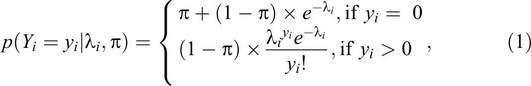
where
The ZIP model has been further developed by many others, for instance, to deal with overdispersion and heterogeneity by incorporating a zero-inflated negative binomial model (e.g., Ridout, Hinde, and Demetrio 2001; Mwalili, Lesaffre, and Declerck 2008), adding additional random effects (e.g., Monod 2014), or both (e.g., Moghimbeigi et al. 2009), and mixing multiple groups (e.g., Lim, Li, and Yu 2014).
Lin and Tsai (2013) further extended the ZIP model to include inflations at both zero and the value k. To illustrate, a response Yi with excessive values of zero and k, the PMF is defined as follows:
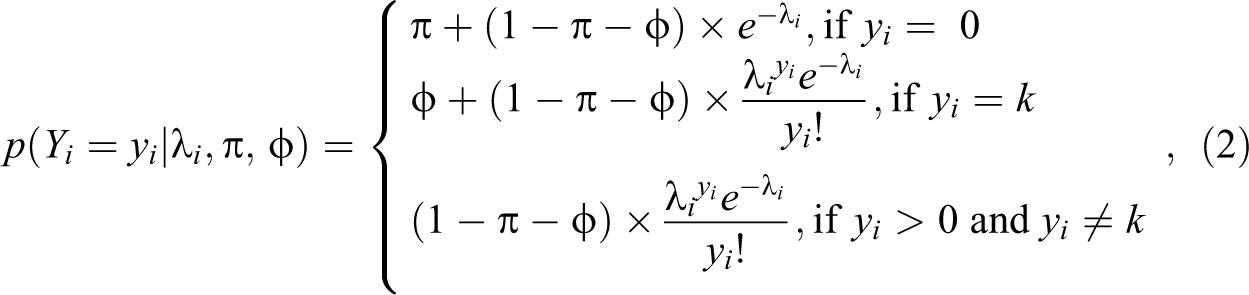
where
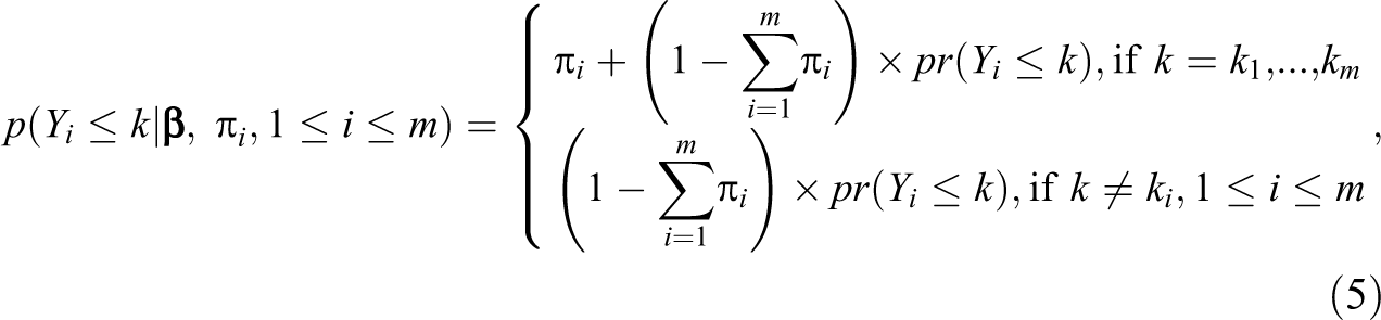
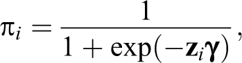
Begum, Mallick, and Pal (2014) suggested a general framework of inflated values for Poisson outcomes. To simplify our notation, we drop the subscript for individuals and use the subscript to differentiate the inflated values. For example, suppose a discrete random variable Y has inflated probabilities at values
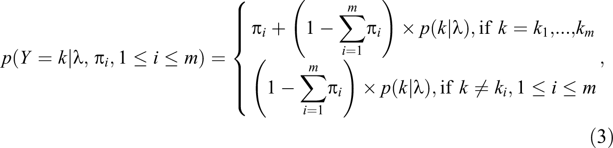
where
For other types of discrete outcomes, such as binary, multinomial, or ordinal, various single value inflated models were developed, including binary choice model with misclassification (Hausman, Abrevaya, and Scott-Morton 1998), zero-inflated Bernoulli model (Diop, Diop, and Dupuy 2016), zero-inflated binomial model (Hall 2001; Vieira, Hinde, and Demetrio 2010), zero-inflated ordered (ZIO) probit model (Harris and Zhao 2007), baseline or zero-inflated multinomial logit model (Bagozzi 2016; Diallo, Diop, and Dupuy 2017), and middle category inflated ordered model (Bagozzi and Mukherjee 2012). Similar extensions have been made to incorporate inflations other than zero for multinomial or ordinal outcomes (e.g., Sweeney, Haslett, and Parnell 2017).
Following Begum et al. (2014), a further generalization could be made if the PMF is replaced by other discrete distributions, for example, multinomial, negative binomial, and so on. For instance, if
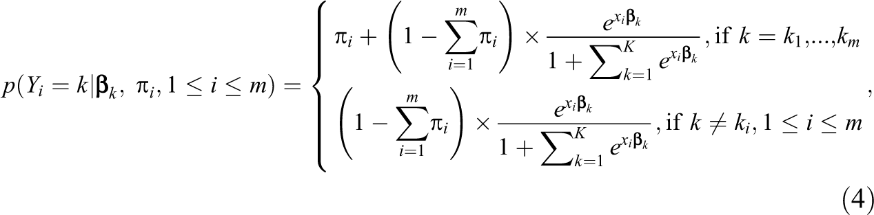
where
where
where
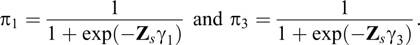
Once the model is specified, the full likelihood function can be constructed. Suppose the random variable Y follows a multinomial distribution with a total of five categories and has the inflated probabilities at the values 1 and 3. Defined
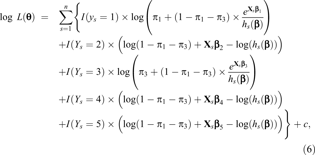
where
The maximum likelihood estimator of
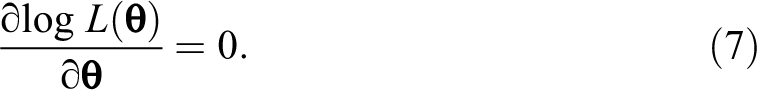
The information matrix can be obtained by taking the second derivatives of the log likelihood. The detailed derivations for the above example and a general k-category multinomial logit model are given in Online Appendix A. Various methods have been proposed to find the solutions for the unknown parameters, for example, method of moments (Begum et al. 2014), direct maximum likelihood (Bagozzi 2016; Begum et al. 2014; Diallo et al. 2017), and maximum likelihood via the expectation−maximization algorithm (Begum et al. 2014; Su et al. 2013). Furthermore, Diallo et al. (2017) provided a rigorous investigation of the maximum likelihood estimator in terms of the identifiability, existence, consistency, and asymptotic normality under classical regularity conditions.
The implementation of the generalized inflated models usually requires users to construct the log-likelihood function and its gradient and then solve the score function by a Newton–Raphson type of algorithm. A direct implementation of maximum likelihood for the five-category example above using the commercial package SAS/IML (1990) is provided in Online Appendix B. To facilitate further use of the generalized inflated models, we also provided an implementation for the direct maximum likelihood method in the commercial package SAS by using PROC NLMIXED (SAS 2013; see Online Appendix C for details). The PROC NLMIXED offers great flexibility in specifying various likelihood functions and powerful capabilities to conduct numerical computations. Not only are standard single-category inflated models (Voronca, Egede, and Gebregziabher 2014) allowed, but multicategory inflated discrete ones as well. In addition, further extension can be easily made to manage clustering due to longitudinal or hierarchical data structures by adding a random effect in the log-likelihood function above.
Monte Carlo Experiments
To evaluate the performance of the maximum likelihood estimator derived above, we conducted a series of Monte Carlo experiments for the multinomial, CL (ordered), Poisson, and zero-truncated Poisson models with two inflated values, for example, at 1 and 3. Four independent variables X
1 to X
4 were generated from uniform U(2,5), normal N(1,1.5), exponential
We considered two scenarios: Case (i)—the probabilities of inflations are fixed and Case (ii)—the probabilities of inflations are covariate-dependent. For Case (i), the inflation probabilities take the value of .05 to .20 by a step of .05. For Case (ii), to see whether the estimation is stable, two additional random variables from normal N(−1,1) and Bernoulli B(.3) were included for the inflation probabilities
The parameter vector of the inflated values was chosen to make the average of inflation probabilities within each sample as .05, .10, .15, and .20, accordingly. Each of experiments was replicated 500 times with a sample size of 3,000. The exemplary code for Case (i) is given in Online Appendix B (SAS/IML implementation) and C (NLMIXED implementation). The results and the rest of codes are available upon request.
In addition to the true model and naive model, both of which ignore the inflations, it is helpful to consider a scenario in which researchers don’t know precisely which categories are inflated. We also estimated models where the inflated categories were incorrectly specified, for example, at values 1 and 4.
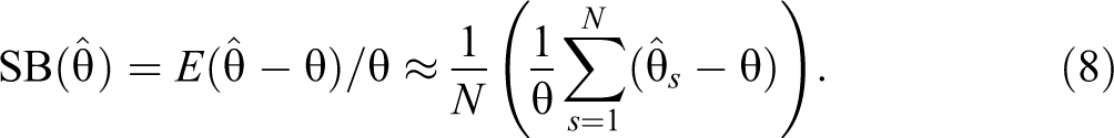
The quality of estimates is evaluated by using the standardized bias, the root standardized mean square error (RSMSE), and the coverage rate (CR). The SB for parameter
The RSMSE for parameter
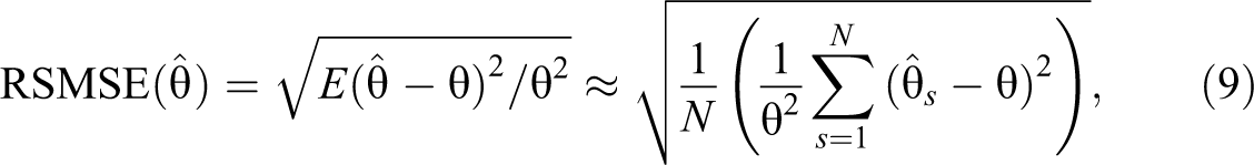
where N denotes the number of replicates;
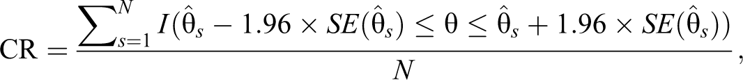
where
Results
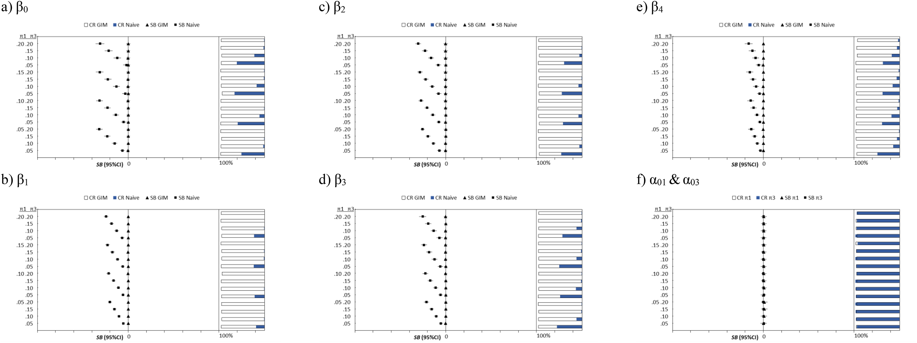
Figure 1 presents the comparison of the estimates between the generalized inflated multinomial (GIM) model and the naive multinomial model for the simulated data for an outcome from “1” to “5,” with inflation at values “1” and “3.” With the reference group at “5,” the second subscript is used to differentiate the categories, for instance, β01 to β04 are estimates for the intercept with categorical data ranging from “1” to “4”; β11 to β14 are estimates for the first independent variable, and so on. Since only category “4” has four predictors, β44 refers the coefficent of X 4 for category “4.”
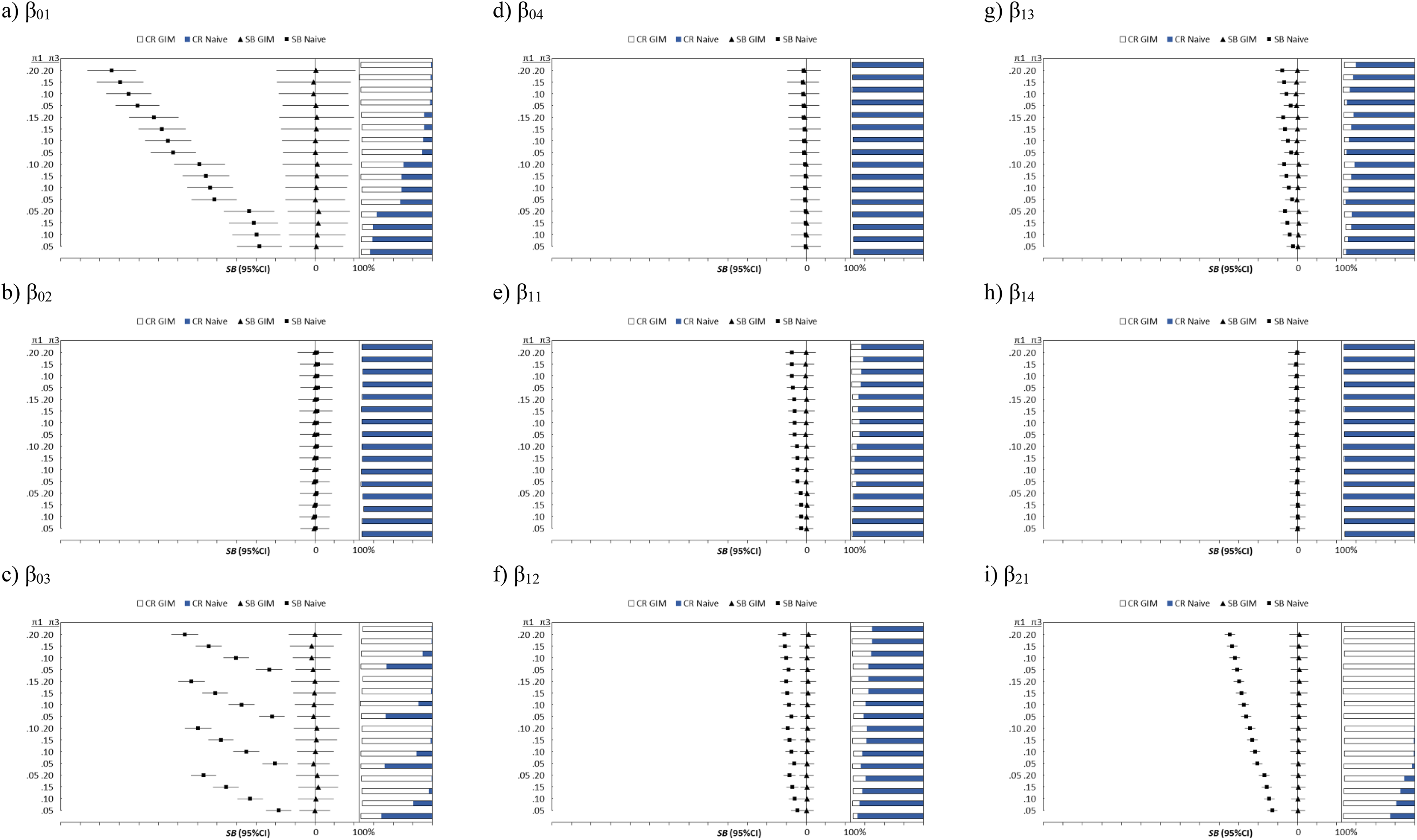
Plots of the SB, RSMSE, and CR of the generalized inflated multinomial model plotted against the fixed π1 and π3. The dot represents the SB, with the RSMSE as the error bar. The horizontal bar represents the CR at each level of π1 and π3. SB = standardized bias; RSMSE = root standardized mean square error; CR = coverage rate.
(continued).
Using the last category “5” as the reference, all estimates obtained from the GIM are unbiased with nearly 100% CR. The CRs were plotted on the right side of each of charts, with the CR from the GIM as the base (white bar) overlapped with the CR from the naive model (blue bar). As expected, the naive multinomial models produce biased estimates of low CRs on the intercepts β01 for the category “1” and β03 for the category “3” as shown in panels (a) and (c). Specifically, a higher value of
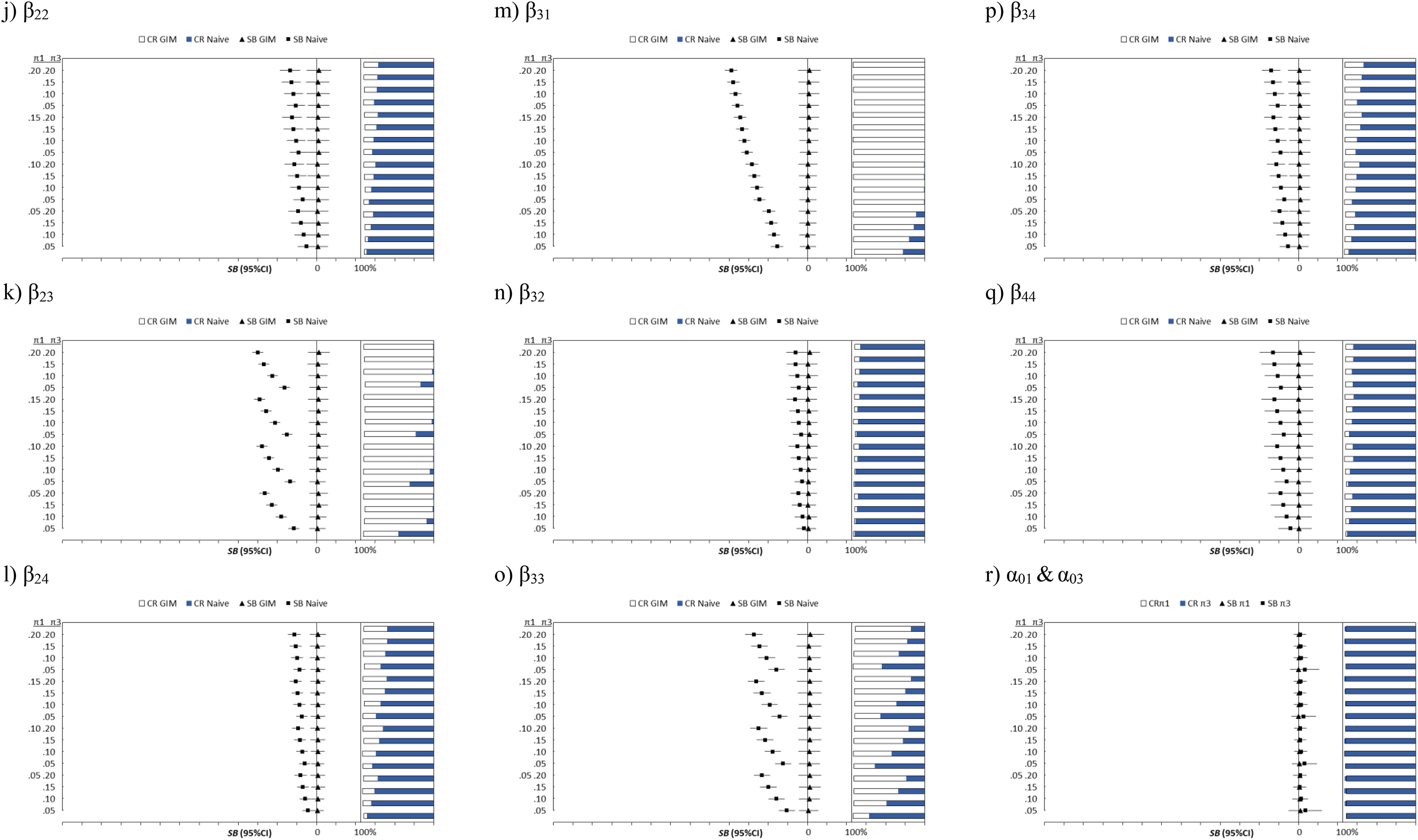
Figure 2 summarizes the performances of the generalized inflated cumulative logit (GICL) model and the naive CL (ordered) models for an outcome of “1” to “5” with inflation at the values of “1” and “3.” Unlike the multinomial case, the naive CL (ordered) models give biased estimates and low CRs for all parameters. Similar to the naive multinomial models, the bias increases with the size of inflated probabilities
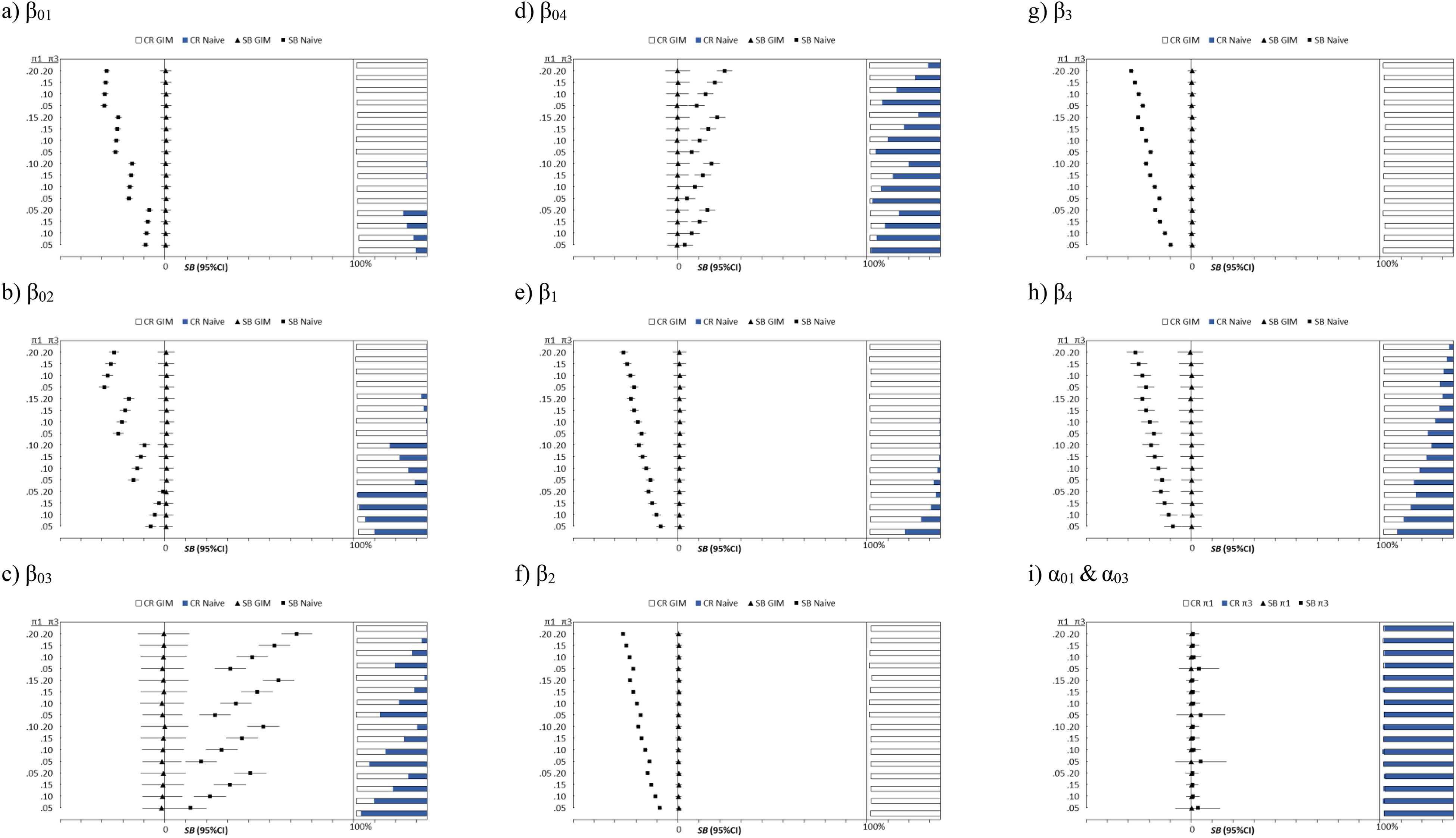
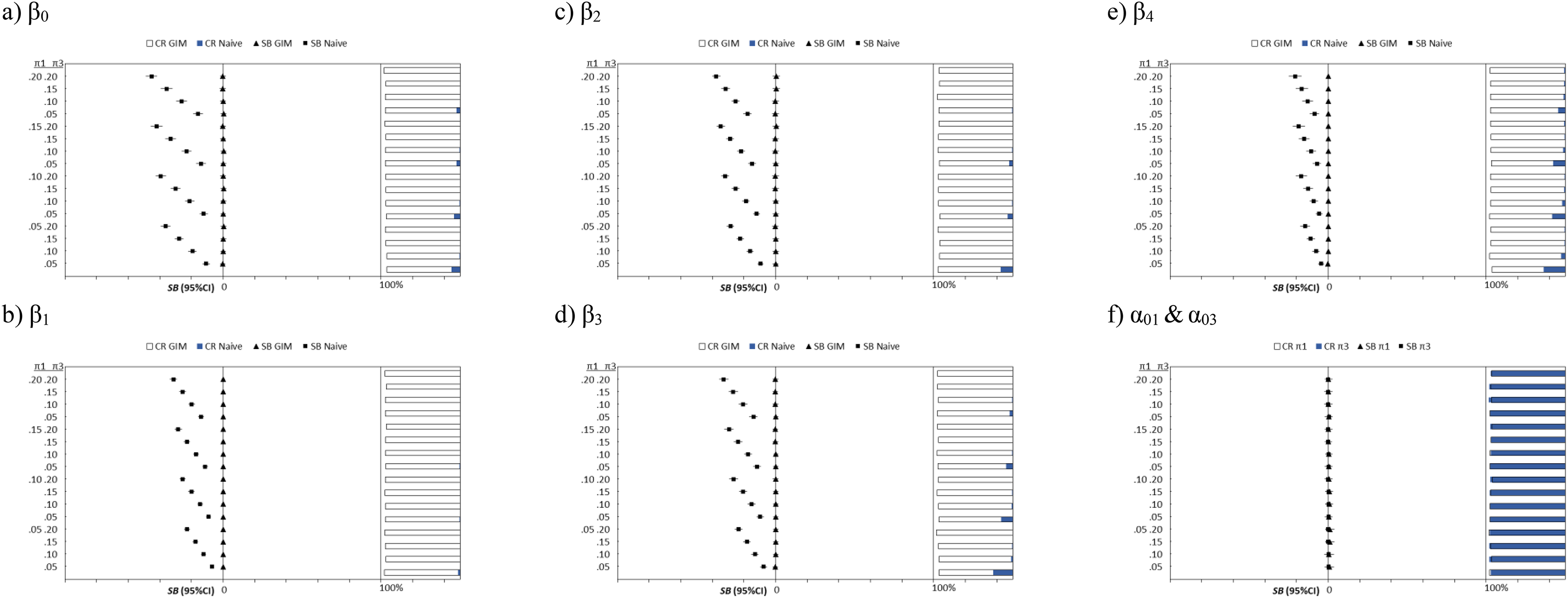
Both Figures 3 and 4 show the exact pattern of biases and CRs for the Poisson and zero-truncated Poisson models: (1) the naive models produce biased estimates and poor CRs but low RSMSEs, (2) the size of bias increases and the CR decreases dramatically as the probabilities of inflation increases, especially for
Plots of the SB, RSMSE, and CR of the generalized cumulative logit model plotted against the fixed π1 and π3. The dot represents the SB, with the RSMSE as the error bar. The horizontal bar represents the CR at each level of π1 and π3. SB = standardized bias; RSMSE = root standardized mean square error; CR = coverage rate.
Plots of the SB, RSMSE, and CR of the generalized inflated Poisson model plotted against the fixed π1 and π3. The dot represents the SB, with the RSMSE as the error bar. The horizontal bar represents the CR at each level of π1 and π3. SB = standardized bias; RSMSE = root standardized mean square error; CR = coverage rate.
Plots of the SB, RSMSE, and CR of the generalized inflated zero-truncated Poisson model plotted against the fixed π1 and π3. The dot represents the SB, with the RSMSE as the error bar. The horizontal bar represents the CR at each level of π1 and π3. SB = standardized bias; RSMSE = root standardized mean square error; CR = coverage rate.
In summary, the estimates obtained from the naive models are not satisfactory with regard to the biasness and the CR—for example, the biases could be as high as 200 percent for intercepts of the inflated categories in the GIM when the inflation probabilities reach a .20 level. Interpretations based on naive estimators could distort the underlying data-generation mechanism. The generalized inflated models, on the other hand, show superiority over the naive models, for example, unbiased estimates (usually less than 5 percent), high CRs, and small RSMSEs.
For Case (ii) where the probabilities of inflation depend on covariates, only the estimates produced by the generalized inflated models are reported because none of the naive models give unbiased estimates. For the multinomial outcomes (Table 1), none of the biases are beyond 5 percent, and most of CRs are higher than 95 percent. In terms of precision, there is no difference between the estimates obtained from the inflation equations and those from the multinomial outcomes. The size of
Simulation Results of the Generalized Inflated Multinomial Model for Case (ii).
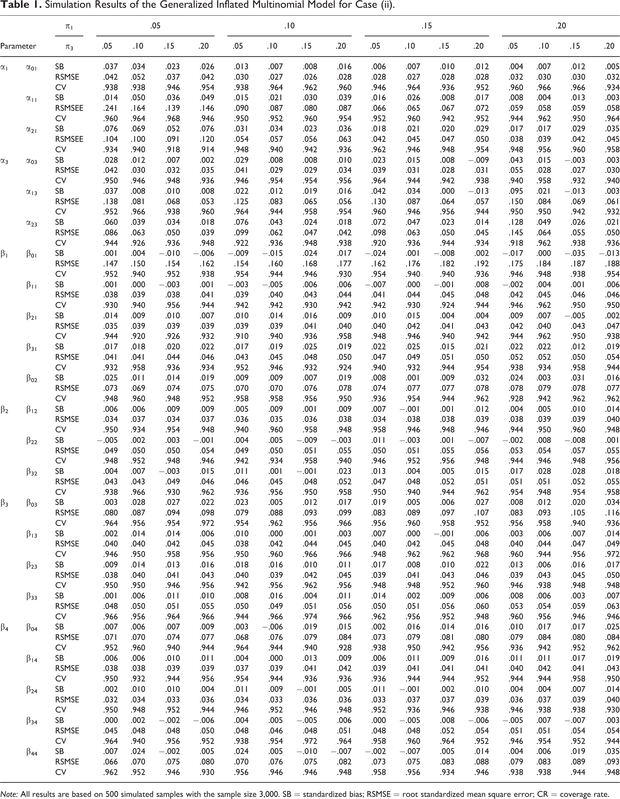
Note: All results are based on 500 simulated samples with the sample size 3,000. SB = standardized bias; RSMSE = root standardized mean square error; CR = coverage rate.
Simulation Results of the Generalized Inflated Cumulative (Ordered) Logit Model for Case (ii).
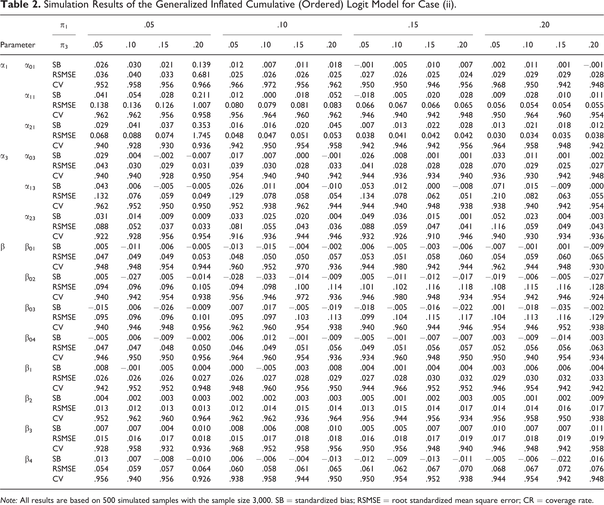
Note: All results are based on 500 simulated samples with the sample size 3,000. SB = standardized bias; RSMSE = root standardized mean square error; CR = coverage rate.
Simulation Results of the Generalized Inflated Poisson Model for Case (ii).
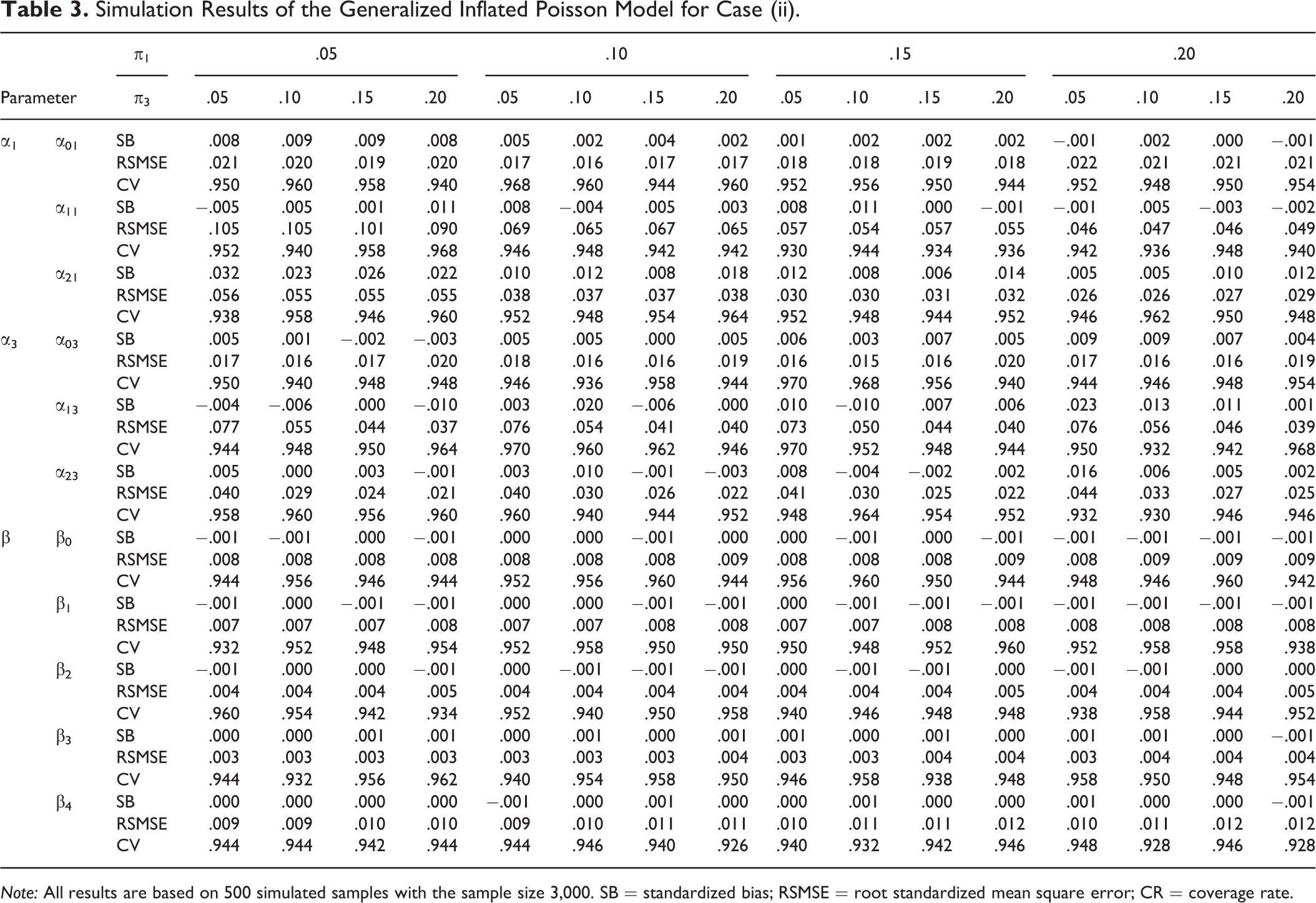
Note: All results are based on 500 simulated samples with the sample size 3,000. SB = standardized bias; RSMSE = root standardized mean square error; CR = coverage rate.
Simulation Results of the Generalized Inflated Zero-truncated Poisson Model for Case (ii).
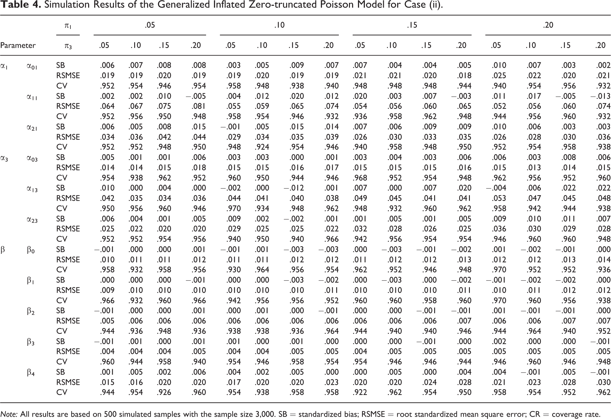
Note: All results are based on 500 simulated samples with the sample size 3,000. SB = standardized bias; RSMSE = root standardized mean square error; CR = coverage rate.
Based on the evaluation for the estimates obtained from the direct maximum likelihood method, the Newton–Raphson type of algorithm seems to provide an efficient way to estimate the generalized inflated models for a moderate sample size of 3,000.
Since the performance of the misspecified models is only slightly better than the naive models with biased estimates and poor CR,
2
to save space, only fit indices for the experiments are given. Begum et al. (2014) suggested using Akaike information criterion (AIC) to find appropriate inflated models among all possible combinations of inflated values based on empirical distribution. Table 5 gives the average AIC for the naive, the misspecified, and the true models by the type of models and the level of inflation. For all experiments, the correct specified models yield the lowest average AIC value. Compared to the naive models, the misspecified ones usually have lower AIC except for a few cases, for example, (i) GIM and (ii) GICL when the inflation probability
The Average AIC by Levels of Inflation Based on 500 Simulated Samples with the Sample Size 3,000.
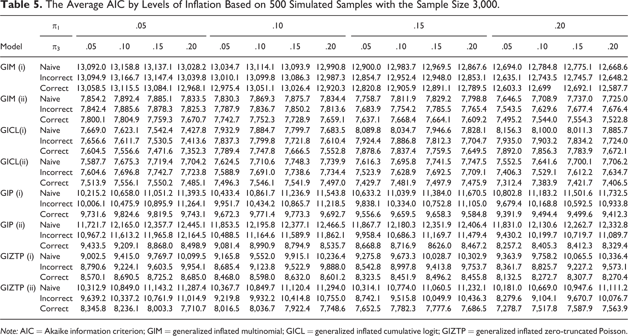
Note: AIC = Akaike information criterion; GIM = generalized inflated multinomial; GICL = generalized inflated cumulative logit; GIZTP = generalized inflated zero-truncated Poisson.
Applications in Health Study
To illustrate the implementation of the generalized inflated models, we fitted a GIP model using the Wave 1 data from the National Longitudinal Study of Adolescent Health (Add Health) study, which is a longitudinal study of a nationally representative sample of adolescents in grades 7–12 in the United States during the 1994–1995 school year (K. M. Harris et al. 2009). The Add Health study was designed as a stratified two-stage cluster sampling in which schools were selected first, and then individuals were selected within the selected schools. The Add Health study provides a rich set of information on respondents’ social, economic, psychological, and physical well-being with contextual data on the family, neighborhood, community, school, friendships, peer groups, and romantic relationships.
Suppose we are interested in smoking behaviors. One measure available in the Add Health is the frequency of smoking, which was recoded from responses for the survey question that asked how many days the respondent smoked in the past 30 days. The responses varied from 0 to 30 and were heaped onto the values ending with 0 or 5. Although there was not a consensus on how to categorize the number of smoking days into patterns, for example, light smoking, moderate smoking, or heavy smoking (Schane, Ling, and Glantz 2010), we grouped the number of days respondents reported smoking cigarettes by intervals of 5, such as 0, 1–5, 6–10, 11–15, 16–20, 20–25, and 25+ (Bjartveit and Tverdal 2005). The distribution was highly skewed with two peaks at the “0” group (73.58%) and the “25+” group (11.60%), which suggests that there may exist inflations on both groups. Several predictors are included: age (continuous, ranged from 11 to 21), female (dummy, coded as 1 if female, 0 otherwise), race (dummy, coded as 1 if African American, 0 otherwise), repeated a grade (dummy, if repeated a grade or been held back a grade, 0 otherwise) and religiosity (dummy, if weekly attended religious services, 0 otherwise).
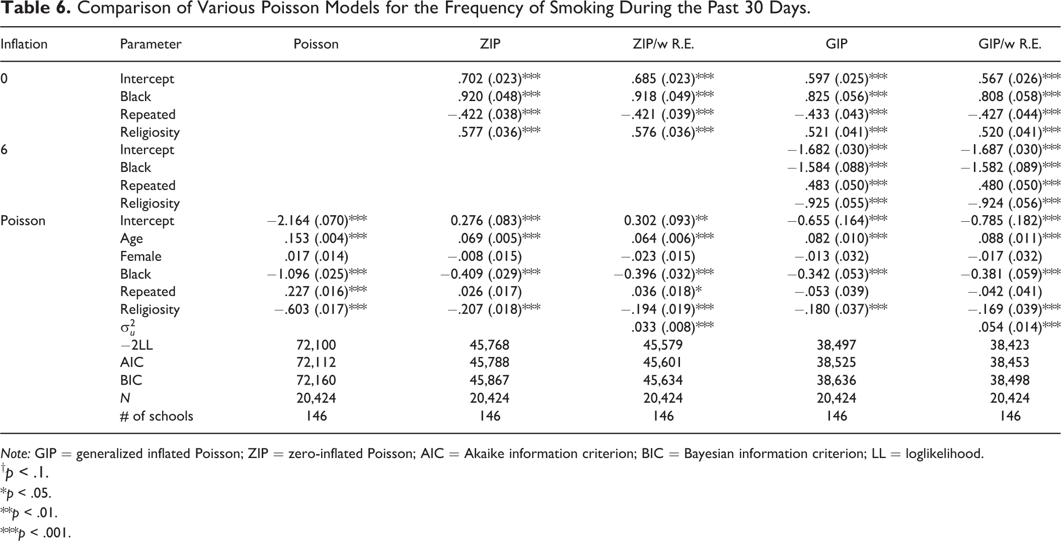
Table 6 reports the results obtained from four different models for the frequency of smoking. Besides the GIP, results from the naive Poisson model, ZIP model, ZIP model with random effect, and the GIP model with random effect are also provided. The naive Poisson model showed a strong positive effect (.227, p < .001) of “repeated a grade” on the frequency of smoking. We conducted the Vuong (1989) test and Clark (2007) test to see if a ZIP model was needed. Both the Vuong statistic (64.89, p < .001) and Clark statistic (7,897.00, p < .001) suggested that a ZIP model should be preferred over the naive Poisson model.
Comparison of Various Poisson Models for the Frequency of Smoking During the Past 30 Days.
Note: GIP = generalized inflated Poisson; ZIP = zero-inflated Poisson; AIC = Akaike information criterion; BIC = Bayesian information criterion; LL = loglikelihood.
† p < .1.
*p < .05.
**p < .01.
***p < .001.
Three covariates were included in the logit of zero inflation—race, repeated a grade, and religiosity. The negative effect of “repeated a grade” suggests that those who repeated a grade are less likely to be in the “0” group. Specifically, the odds of being in the “0” group for one who repeated a grade is reduced by nearly 35 percent (1 − exp(−.442)). Similar to the ZIP, the variables of black, repeated a grade, and religiosity were added to the logit for the inflation of the “25+” group for the GIP model. The strong positive coefficient shows that those who repeated a grade are 1.68 times (exp(.521)) as likely as those who did not repeat a grade to be in the “25+” group. Interestingly, the coefficient of “repeated a grade” in the Poisson part of the ZIP and the GIP models turned out to be not significant, which reveals that the positive effect of “repeated a grade” might be driven by the inflated parts. To address the possible clustering among the respondents within each of the schools, we added a random effect on school level for the ZIP and the GIP models. The significant variance of the random effect implies a clustering effect on the frequency of smoking within each of the schools.
Comparing the fit indices among the ZIP model, the ZIP with random effect, the GIP model, and the GIP model with random effect, the GIP model shows much smaller values of AIC and Bayesian information criterion (BIC) than the ZIP model, while the GIP model with random effect further improves the model fitting.
In the Add Health, another measure of smoking behaviors is the number of cigarettes smoked each day, which can be used as an example of the generalized inflated models for ordinal responses. Similar to the smoking frequency, we grouped the number of cigarettes smoked each day by an interval of 5, such as 0 (never), 1–5 (light, coded as 1), 6–10 (mild, coded as 2), 11–15 (moderate, coded as 3), 16–20 (heavy, coded as 4), and 20+ (severe, coded as 5; Farrell, Fry, and Harris 2003). Most of the responses concentrated on the never (74.31%) and light (16.06 percent) categories. Table 7 presents the results obtained from the CL (ordered) model, the ZIO logit model, and the GICL with inflations on never and light categories using the last group severe as reference. To be consistent with the previous Poisson models, the same set of independent variables for the regular model parts was used, but for the inflation parts, “black” was replaced by “female” to avoid numerical issues we encountered in the exploratory analysis. The value of AIC shows that the GICL is preferable among the three, while the ZIO would be preferred if BIC is used. It is worth noting that the estimated intercept for the never group is not significant for the CICL. This suggests that the model specification for the inflation parts or distribution assumption might not be appropriate.
Comparison of Various Cumulative (Ordered) Logit Models for the Quantity of Smoking During the Past 30 Days.
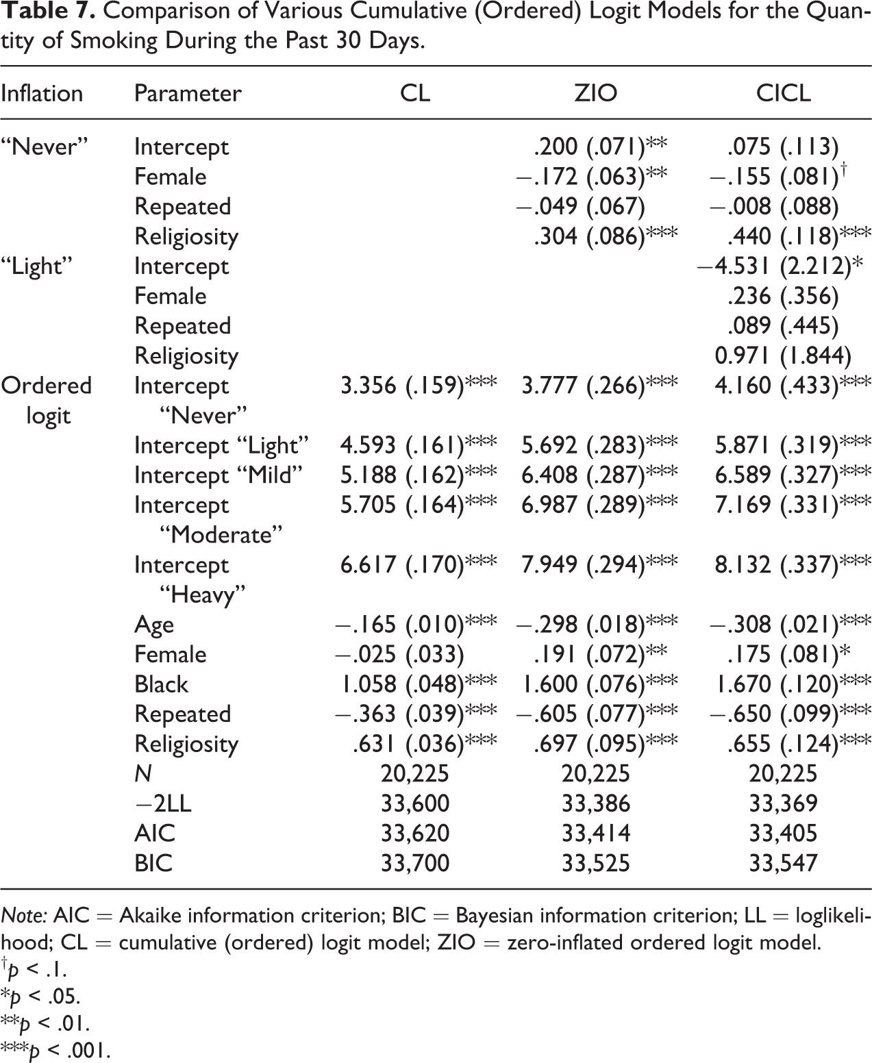
Note: AIC = Akaike information criterion; BIC = Bayesian information criterion; LL = loglikelihood; CL = cumulative (ordered) logit model; ZIO = zero-inflated ordered logit model.
† p < .1.
*p < .05.
**p < .01.
***p < .001.
Conclusion
Due to various reasons, variables from survey studies have inflations on certain values that may lead to biased estimates and incorrect inference if not treated properly. The current study integrated the existing literature on the single-value inflated models and developed a general framework to handle variables with more than one inflated value. We provided a general implementation with maximum likelihood estimation. To assess the performance of the maximum likelihood estimation, we conducted simulation experiments to evaluate the procedure for the multinomial, ordinal, Poisson, and zero-truncated Poisson outcomes under a range of scenarios, for example, different levels of inflated probabilities, and whether covariates are included.
We found substantial bias and poor inference for the naive models—not only for the intercept(s) of the inflated categories, but other coefficients as well. Specifically, with higher values of inflated probabilities, the naive models produced larger bias and lower CR—since the confidence intervals were too narrow to cover the true parameter. Although in many cases the biased estimates on the intercept(s) of the inflated categories might not be a major concern, ignoring the inflations introduces bias and leads to incorrect inferences for almost all the parameters included in a model. More importantly, doing so also distorts the mechanism that generates the data. Generally speaking, the maximum likelihood estimation performs well for all the models discussed in this study with unbiased estimates and satisfactory coverages, even when the number of parameters that need to be estimated is quite large.
Nevertheless, the proposed model has some limitations. First, to facilitate implementation, the inflated values need to be known in advance. Begum et al. (2014) proposed a three-step modeling strategy that estimates all possible combinations of the GIP models among the empirically observed values with high frequencies, and then, analysts evaluate the models by their goodness-of-fit indices, for example, χ2 statistic and AIC. The estimates in the final model are assessed by asymptotic t-test statistics. Although the Vuong test or Clarke test has been widely used to evaluate between Poisson and ZIP models, a formal test is still needed for the generalized inflated models. Another possible strategy is to partition the sample to training and testing sets if the sample size is sufficiently large and use the testing set to evaluate whether the model specification on the inflations is reasonable. Secondly, to avoid numerical issues, cautions should be taken regarding the variables included in the logit of the inflated probabilities. For example, it has been suggested that at least one of the covariates included in the regular Poisson part needs to be excluded from the logit for the zero inflation for a ZIP model, or vice versa, to prevent the possible numerical difficulties (Diop, Diop, and Dupuy 2011; Staub and Winkelmann 2013). For a zero-inflated multinomial model, Diallo et al. (2017) proposed to run a variable selection using a Logistic model for a binary indicator of whether the response is zero and then use the resulting variables as candidates for the logit of zero-inflated probability. Acknowledged by Diallo et al., 2017 this procedure is not a precise one because some of the zeros actually belong to the multinomial part of the model. It is possible to mimic the procedure for each of the inflated values, but it would be more appropriate if a simultaneous selection procedure is developed. Furthermore, by taking advantage of the flexibility of the NLMIXED procedure, the current study demonstrates an example of GIP with a random effect. Future work is desirable to extend it for multiple random effects or longitudinal structures. In addition, the current study adopted a mixed method that used a logit model for the inflated probabilities without further elaborating the mechanism of inflation. Previous studies have shown that the inflation or heaping on certain values may be due to rounding to nearby popular values (Crawford et al. 2015; Wang and Heitjan 2008). We hope that the current work can stimulate further developments that incorporate various measurement models.
Supplemental Material
Supplemental Material, appendix - Generalized Inflated Discrete Models: A Strategy to Work with Multimodal Discrete Distributions
Supplemental Material, appendix for Generalized Inflated Discrete Models: A Strategy to Work with Multimodal Discrete Distributions by Tianji Cai, Yiwei Xia and Yisu Zhou in Sociological Methods & Research
Footnotes
Authors’ Note
Views expressed are those of the authors.
Declaration of Conflicting Interests
The author(s) declared no potential conflicts of interest with respect to the research, authorship, and/or publication of this article.
Funding
The author(s) disclosed receipt of the following financial support for the research, authorship, and/or publication of this article: This work was partially supported by the Multiple Year Research Grant (ref: MYRG2015-00005-FSS) funded by RDAO, University of Macau.
Supplemental Material
Supplemental material for this article is available online.
Notes
References
Supplementary Material
Please find the following supplemental material available below.
For Open Access articles published under a Creative Commons License, all supplemental material carries the same license as the article it is associated with.
For non-Open Access articles published, all supplemental material carries a non-exclusive license, and permission requests for re-use of supplemental material or any part of supplemental material shall be sent directly to the copyright owner as specified in the copyright notice associated with the article.