A Cautionary Note on the Reliability of the Online Survey Data: The Case of Wage Indicator

Representativeness of the Online Data

One of the issues that are most often raised by researchers is representativeness of the sample, a problem that is particularly acute in the case of volunteer surveys (Couper 2000). In spite of Internet’s increasing penetration, access to the Internet is still unequally distributed. In some countries, individuals with lower earnings might be underrepresented among Internet users. Similar arguments might be put forward in the case of elderly or less educated individuals. While in the developed world, these concerns might play a smaller role, in developing nations, they cannot be ignored (James 2008; Tijdens and Steinmetz 2016). Even in the cases where surveys reach entire targeted population, nonresponse might be larger in the case of Internet-based surveys due to technical issues, such as the lack of a stable connection or insuficient time to complete the survey, among others. Finally, one should consider that individuals of different groups might have different preferences concerning Internet use (e.g., Chen 2014; Steinmetz et al. 2013).

An alternative approach to explore the bias from online surveys relies on dual databases, that is, databases that contain two modules: one administered to a representative sample of the population and a web-based module. Bandilla, Bosnjak, and Altdorfer (2003) is an early example of this type of analysis, as authors compare two samples of the ISSP in Germany. They show that participants differ significantly with regard to sociodemographic structure and in other relevant variables. Even after weighting, results were inconsistent across samples. However, when they repeated the procedure within educational categories, differences in descriptive statistics disappear. By contrast, Schonlau et al. (2009) show that the use of propensity score matching weights improves the fit between the representative and the web-survey based components of the U.S. Health and Retirement Study, though some differences remain. Differences in distributions between samples from web-based surveys and traditional, representative surveys were also observed in the American National Election Study (Malhotra and Krosnick 2007) and in two similar surveys (one conducted via Internet, second as face-to-face interview) in Belgium (Loosveldt and Sonck 2008).

The Case of WI

Utilizing experience from the other online surveys, WI appears to be particularly concerned with the quality of the collected data and the outreach to the relevant population. Indeed, WI data are collected by experienced researchers and with great attention to methodological prudence; hence, their quality is possibly much better than ad hoc surveys in many countries as well as quasi-commercial data on wages from various wage comparison/ranking tools. WI data are collected through multilingual websites, one for each participating country. In some countries, WI also provides websites targeted toward groups such as women, specific professional groups, and so on. ⁸ Websites that offer WI survey have to fulfill a “quality of information” criteria set by the nongovernmental organization operating WI. These websites rank high in search engines for a wide array of key words. Hence, WI recruitment is based mainly on voluntary participation by individuals suficiently interested in related topics to query one of the related key words in the search engine. In addition, many specialized service providers—for example, job brokers, temporary work agencies—advertise the tools offered by WI.

Recognizing the risk of satisficing (see Sue and Reiter 2012), WI survey is short and only few questions are actually obligatory to the participants. Moreover, participants are incentivized to complete the survey, both because they can get a more accurate SalaryCheck data and they get a chance to obtain a monetary prize equal to the weekly minimum wage, monthly in the case of countries with low minimum wages. Chances are doubled for participants willing to become part of a panel survey. ⁹ The standard version of the survey requires approximately 10–20 min to complete, but in countries with slower average speed of Internet, this survey is further shortened to roughly 5 min (Tijdens et al. 2010). Finally, the survey can be completed in several sessions within a week span.

Given the extensiveness of the WI data in terms of breadth and coverage, earlier literature on the data project asks whether WI data are reliable enough to be used for research purposes. In analyses for Germany and the Netherlands, Steinmetz et al. (2009) and Steinmetz and Tijdens (2009) compare the WI data to nationally representative databases, the German Socioeconomic Panel and the Labor Supply Panel from the Netherlands. They find that in both cases, WI samples are not representative of the general population. Consequently, wage distributions differ between the two types of the sources, yielding biased estimators in the case of online sources vis-à-vis the representative sources.

In summary, previous findings consistently report differences between the representative and the web-collected surveys. The use of weights to improve the fit between the samples presents a mixed record in terms of balancing the data from online surveys. The main limitations of the previous literature concern both methodology and the coverage. In terms of methodology, the construction of weights does not assure balancing and necessitates access to both WI and benchmark data, as both WI and benchmark samples are reweighted. In terms of coverage, the reliability analyses are available for selected countries and years. Against this background from the earlier literature, our analysis contributes to both the methodological and the cross-country dimensions of the WI. We test a novel procedure for balancing WI data to nationally representative benchmark samples. This new approach assures balancing and reweights only the WI sample, which makes it a convenient addition to the raw WI data for all researchers interested in making a relevant WI sample resemble a representative population despite lack of access to a representative sample. Wide country coverage allows researchers to explore more systematically the reasons behind WI representativeness or lack thereof. While in a strict sense, we can only comment on the actual 95 data sets that we use in the analysis, the broad coverage of countries, years, and various sources of data lends some grounds to cautious generalizations of our results.

Comparing the Distributions

The principal interest lies in testing if data from two sources come from the same distribution. This analysis poses two important challenges. First, the sample sizes in the two sources may differ substantially. Second, self-reported data, such as WI or LFS, are likely to contain more round numbers, whereas administrative sources, such as structure of earnings survey, are likely to contain exact gross wages, which are rarely round. These two challenges necessitate that the tests to be employed make no assumptions about the underlying distribution of the data. Such requirement yields three candidate tests to compare the two samples: Kolmogorov–Smirnov test, Mann–Whitney U test, and Epps–Singleton two-sample test. These three tests share the null hypothesis that both analyzed samples are drawn from the same population. However, the power of the tests varies.

The Kolmogorov–Smirnov test (Kolmogorov 1933; Smirnov 1933) is the most widely used among the three, and it is based on a comparison of the cumulative distribution function in the two samples. The test statistic is proportional to the maximum discrepancy between the two samples. This test is sensitive to differences in the median, the shape, and the span of the distributions. It permits the use of survey/sample weights. However, its properties rely heavily on the assumptions of continuity of the distributions (the distributions should be fully specified). Moreover, it tends to be less sensitive if the discrepancy occurs in the upper tail of the distribution.

The Mann–Whitney U test (Mann and Whitney 1947) follows a different approach. Instead of comparing cumulative distribution functions, it ranks all observations. Under the null hypothesis, that the two samples came from the same population, the ranks will be randomly distributed between the two samples. This implies that this test is better to capture changes in the location of the distribution, which are usually reflected at the median. In addition, Schmid and Trede (1995) demonstrated in a Monte Carlo experiment that if wages follow a Pareto distribution, the Mann–Whitney U test is more powerful than Kolmogorov–Smirnov. ¹¹

Finally, the Epps–Singleton (1986) test is based on the empirical characteristic function. When compared to the Mann–Whitney U test, the main advantage of Epps–Singleton lies on its ability to detect discrepancies in the location, family, and scale (Goerg, Kaiser, and Bundesbank 2009). When compared to Kolmogorov–Smirnov test, Epps–Singleton has two advantages. First, it is more flexible since the characteristic function is completely defined for discrete and continuous data. Second, it tends to be more powerful (Goerg et al. 2009).

Given the advantages and disadvantages for each test, we employ all three, adapting them to accommodate for sample weights. We provide systematic tests for each analyzed sample, with the null hypothesis that both WI sample and the alternative sample are drawn from the same population. We provide these tests for the raw WI data as well as for the WI data after applying the reweighting procedure as described below.

Reweighting Procedure

If tests reject the null hypothesis that data come from the same underlying distribution as the population, then suitability of the nonrandom sample from the population for reliable statistical inference without any further correction becomes questionable (Valliant and Dever 2011). A possible solution to this problem is to reweight observations in the WI to make them resemble representative data. Steinmetz et al. (2009) use (the inverse of) the estimated propensity scores as weights. ¹² Formally, the procedure involves running a probit/logit regression where the explained variable is the source (a binary variable that takes the value of 1 when an observation comes from benchmark data and 0 otherwise). Then, one may define w i = 1 / ( 1 − P B ( X i ) ) for observations from the WI and w i = 1 / P B ( X i ) for observations coming from the benchmark sample, where P B denotes the predicted probability from the estimation, otherwise called the propensity score. ¹³ Inverse propensity score (IPS) weighting schemes give large weights to observations in WI survey that are very unlikely to be present in this sample and small weights to the observations that are frequent in this sample. We refer to these weights as IPS. By definition, such reweighting scheme cannot balance data from WI vis-à-vis a benchmark representative data, as it does not link relative frequencies between the two samples. For balancing to be achieved, procedure has to give higher weights to those observations that are common to both samples (conditional on characteristics) and a smaller weights to values specific for WI and rare in representative samples (conditional on characteristics). Moreover, Huber (2011) shows that weights constructed as inversed probabilities are more sensitive to a misspecification of the propensity score than alternative approaches, which rely on employing a matching estimator once the propensity score is obtained. Indeed, stratification is one of the matching estimators, but a relatively low-powered one (see the characterization of the available matching estimators by Caliendo and Kopeinig 2008).

Moreover, the estimation of the propensity score with the use of the probit/logit maximum likelihood estimation is in fact inferior to alternative methods, in particular, in the case of nonrandomly missing data (e.g., simulation and data examples from Imai and Ratkovic 2014). Hence, a better solution is to rely on moment-based estimation in obtaining the propensity score. This approach was proposed by Imai and Ratkovic (2014) and yields propensity scores that, by construction, balance the covariates, hence the name covariate balancing propensity score (CBPS) matching. The procedure is immune to the propensity score misspecification problem, as it exploits the dual nature of the propensity score as a covariate balancing score and the conditional probability of assignment to subsample. ¹⁴ Imai and Ratković (2014) notice that estimating the propensity score via maximum likelihood, as used typically, can be conveniently rewritten as a transformation of the sample moment conditions for the covariates that are used to obtain the propensity scores. In other words, the propensity score can be thought of as the (non)linear combination of individual characteristics that maximizes the probability that observations are correctly assigned to a subsample. Hence, one can recover weights that produce an exact balance of covariates, in our case—between the WI and the benchmark representative samples.

Conveniently, the derivation of the propensity score via moment-based estimation also gives clear interpretation for the theoretically warranted specification of the weights. Recall, that earlier studies used IPS, which by definition cannot balance samples from benchmark and WI data. In contrast, we rely on the theoretical result of Imai and Ratkovic (2014) and provide the weighting scheme which adjusts data from WI to reflect the structure of the sampling design used in when obtaining the benchmark sample. Specifically, the weights imposed on benchmark representative samples are equal to 1 for all observations in this data (conditional on utilizing survey weights in estimating the propensity score). Adapting Imai and Ratkovic (2014), this necessitates the following weights for the WI data:

where N denotes total number of observations from WI and benchmark representative data, N_B denotes the number of observations in the benchmark representative data (B), and P_B (X_i ) indicates the score for an observation i, obtained using the moment based approach offered by Imai and Ratkovic (2014). This score is analogous to the probability that observation i was obtained from the benchmark sample, given its characteristics.

A conventional alternative to matching using CBPS is the maximum likelihood estimation of propensity scores with subsequent use of balancing weights. Given typically large sample sizes of the benchmark representative data relative to WI data sets, kernel weights appear as superior. ¹⁵ With kernel density (KD) matching, the weights for particular observations represent the distance between its propensity score and the scores of the observations from the benchmark sample. Formally, we follow Smith and Todd (2005) and Morgan and Harding (2006) and calculate the weights as:

where G ( . ) is a kernel function, P j ( X ) are conventionally estimated propensity scores, that is, the conditional probability that an observation comes from a sample j, given its characteristics, where j stands for WI data or the benchmark data; finally, a n is the bandwidth parameter. Smith and Todd (2005) demonstrate that the results of the matching exercise are not dependent on the selection of this parameter (see the recent overview by Imbens and Wooldridge 2009) nor on the functional form of the bandwidth, at least within reasonable limits. The algorithm for bandwidth selection follows Silverman (1986).

KD weights display two main advantages relevant to our context. First, they do not require the researcher to make any arbitrary restrictions on how many and which observations to select from the control group. In fact, the computation of weights happens automatically for all observations. This leads to the second advantage of using the KD weights: A computed weight is a synthetic measure for each observation from WI of how similar it is to all observations from a representative sample. Thus, risk associated with bad matches is minimized, while each observation from WI may be included in subsequent analyses.

Clearly, one would want to balance WI and the benchmark representative data on the same variables, as are part of the sampling design for the benchmark representative samples: place of residence, age, and gender. However, information on place of residence is often missing in WI or is reported in a way that does not permit straightforward comparison with the benchmark representative data sets. ¹⁶ Also, our interest in this article lies in salaries. Hence, we decide to include education in addition to age and gender in the matching procedure. While other human capital variables are asked for in the WI surveys—such as tenure, experience, occupation, or industry—the proportion of missing values for these variables is much larger, a problem shared with many benchmark samples. Their inclusion as additional covariates would have led to a significant reduction in the sample size from the WI, and therefore we confined the matching variables to the most widely accessible. Summarizing, we use age, gender, and education to obtain both weights: conventional propensity score with kernel matching and CBPS.

Testing for the Bias After Reweighting

We perform an Oaxaca–Blinder-type decomposition as operationalized by Jann (2008) ¹⁷ on a Mincerian wage regression. We decompose the difference between WI and each benchmark sample into a part that is attributable to differences in individual endowments between the two data sets, also known as “explained’’ component, and a part that remains attributable to differences in the coeficients when wage regressions are estimated separately for each data set. This second term is the “unexplained’’ component. ¹⁸ Since this decomposition is based on a regression approach, the use of weights is nonproblematic. ¹⁹

Performing an Oaxaca–Blinder decomposition has two main advantages. First, it provides an additional test of the quality of the balancing: A successful balancing implies that differences in characteristics should vanish in statistical terms. This is equivalent to stating that the explained component of the difference between wages from benchmark data and WI should be negligible. Hence, all the difference should be related to the unexplained component, that is, to differences in coefficients. Second, the Oaxaca–Blinder decomposition allows distinguishing the contribution of each of the covariate to total differences in the coeficients, thus making it possible to identify the sources of the eventual differences between WI and the benchmark samples. ²⁰

An issue that arises with the use of Oaxaca–Blinder decomposition is the choice of the structure of wages to be considered as counterfactual for testing the hypotheses on the obtained parameters. We use the parameters from the benchmark samples. This choice is motivated by the key research question behind our article. Thus, the counterfactual represents the wage that participants of the WI would have recorded in the benchmark samples if their characteristics were valued according to the same schedule as in benchmark samples. ²¹ Hence, a decomposition of the following form is run on reweighted data:

where X denotes the individual characteristics (i.e., age, gender, and education). In this approach, β denotes the estimated coeficients of the Mincerian wage regression of the form: ln wage = β X + ε . This regression is estimated for the WI (denoted by WI ) data and for the reference data set of the benchmark representative data (denoted by B ) for each country, year, and occasionally, when more than one nationally representative source is available, also for the source. If the WI data had the same representative features as the benchmark data sets, one would expect the difference ln wage ˆ WI − ln wage ˆ B to be equal to 0 in principle. However, it may also occur that the differences in (mean) wages stem from differences in characteristics and once these are accounted for, there is no difference between the two conditional distributions of wages (i.e., conditional on individual characteristics). Then, the second term in equation 3 should be equal to 0 and estimates of β obtained in the WI data would be just as reliable as the estimates from the benchmark representative data for the analyzed countries.

Differences in Wages Before Reweighting

Wage distributions from WI are in a vast majority of cases different from the distributions in the nationally representative data as documented in Table 1. One obvious way to compare the two data sets is a simple statistic for the means from the two distributions to be equal. These tests show that 11 samples of 95 have statistically similar means. However, such tests are unable to capture differences at other points of the wage distributions. We proceed to complement them with the tests described in Method section. These results confirm that (hourly) wages in WI and nationally representative data differ in statistical sense. In fact, we reject the null hypothesis of wages coming from the same distribution in more than 95 percent of the cases. Rejection rate is actually within what it was expected for significance test with 5 percent confidence level.

OPEN IN VIEWER

Table 1.

Tests for Equality of the Wage Distributions for WI and Benchmark Data.

Test Result	Kolmogorov–Smirnov		Mann–Whitney U		Epps–Singleton
	Wage	Hourly Wage	Wage	Hourly Wage	Wage	Hourly Wage
Do not reject H0	3	2	6	3	1	2
Reject H0	92	90	89	89	92	90
N	95	92	95	92	93	92

Note: The table presents predicted differences in (log) median hourly wages between Wage Indicator (WI) and nationally representative samples. Predicted values come from a regression where the dependent variables is the difference in average hourly wages as a percentage of hourly wages in the representative sample. Values above 1 indicate higher wages being reported in WI. Regression also includes controls for country and source. Regression does not control for differences in characteristics between respondents of WI and nationally representative samples. H0 = null hypothesis.

With WI becoming more recognized and more reliable, one could expect that the rejections of the null hypothesis become more unlikely. To test explicitly this hypothesis, we estimate a model with the mean difference between WI and benchmark data as an explained variable. ²⁶

The set of explanatory variables contains nothing but fixed effects for country, data source, and year. Hence, we may obtain conditional predictions of the difference for the consecutive years covered by WI that are “clean” of the country specificity and data source specificity. The results are reported in Figure 1 in the form of the conditional predictions with confidence intervals of 95 percent. Points below the zero line correspond to mean hourly wages in WI short of analogous value in benchmark nationally representative data. Time trends display no specific pattern. In fact, the differences in mean hourly wages tend to be large at all times, despite substantial increase in WI sample sizes.

OPEN IN VIEWER

Figure 1.

Hourly wages: Distribution of differences between Wage Indicator (WI) and benchmark data. Figure presents predicted differences in (log) median hourly wages between WI and nationally representative samples. Predicted values come from a regression where the dependent variables is the difference in average hourly wages as a percentage of hourly wages in the representative sample. Values above 1 indicate higher wages being reported in WI. Regression also includes controls for country and source. Regression does not control for differences in characteristics between respondents of WI and nationally representative samples.

As noted at the beginning, differences in wages could be a reflection of differences in sample composition. As suggested in the literature, differences in Internet access coupled with preferences of the individuals concerning its use could result in WI samples characterized by relatively younger and better educated individuals. To identify sources of differences, we estimate the mean values of several characteristics of interest (age, education, and gender) on country, source, and year fixed effects. Fitted values for the latter are plotted in Figure A1 in the Online Appendix. ²⁷ In the case of age, differences appear to be widening over time: recent waves of WI are on average 5–10 years younger than those in the representative sample. Similarly, we observe that participants in the WI are on average better educated, as the proportion of respondents with only primary studies is smaller in virtually all cases. Since the selectivity patterns appear to be systematic, we move now to balancing the WI samples to resemble nationally representative distributions in terms of human capital characteristics: age, gender, and education.

Balancing WI Data

We employ three key human capital indicators: gender, age, and education. We make sure that the sample design of the benchmark nationally representative data is reflected in which observations from WI are used. For example, if samples of SES and EUSES cover private employers with nine or more employees, full-time equivalent, we exclude individuals who do not meet these criteria from the WI data prior to matching. Hence, in those cases, we work with a subpopulation of WI rather than the complete data set.

We balance the distributions using the two approaches discussed earlier: Imai and Ratkovic (2014) estimator and KD matching estimator. To facilitate comparison, we provide tests also for the raw (unweighted) distributions and for the weighting scheme suggested by Steinmetz et al. (2009). The results are reported in Table 2, portraying the summary of variable-by-variable, pair-by-pair testing of balancing. ²⁸ The results reveal that, in principle, WI and nationally representative data differ substantially, which was hinted already by Figure A1 in the Online Appendix. Then, the method proposed by Steinmetz et al. works to some extent with the ISSP data but in some cases may actually reduce the balancing. Weights derived from KD matching on a propensity score similar to Steinmetz et al. do better for the ISSP data, balancing majority of these samples. Admittedly, it is not as effective for other sources of data. Finally, our preferred weighting scheme, based on CBPS, is able to balance all the sources of the data. This result is embedded in the estimation method and thus should come as no surprise; but, in the context of the other methods, it shows the improvement in balancing that may be achieved by changing how weights are computed.

OPEN IN VIEWER

Table 2.

Balancing of the Characteristics Between Wage Indicator and Benchmark Nationally Representative Data.

Source	No Balancing			IPS Weights			Kernel Density Weights			CBPS
	None	1 or 2	All	None	1 or 2	All	None	1 or 2	All	None	1 or 2	All
BHPS	0	0	4	0	0	4	3	1	0	4	0	0
EUSES	0	4	13	0	2	15	0	2	15	17	0	0
GSOEP	0	0	4	0	0	4	1	3	0	4	0	0
ISSP	0	7	58	1	19	45	32	22	19	65	0	0
Others	0	9	24	0	2	31	0	7	26	33	0	0

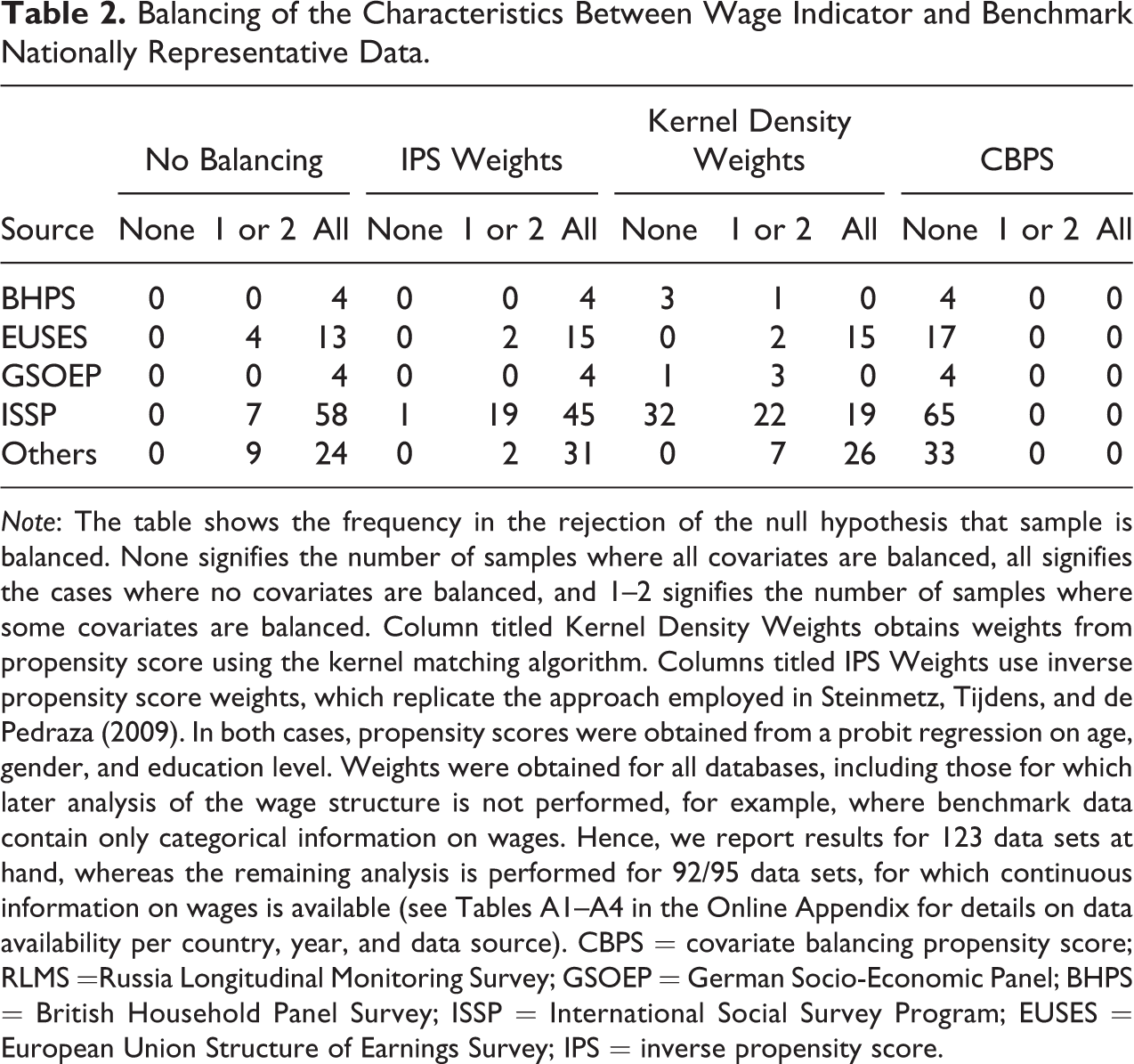
Note: The table shows the frequency in the rejection of the null hypothesis that sample is balanced. None signifies the number of samples where all covariates are balanced, all signifies the cases where no covariates are balanced, and 1–2 signifies the number of samples where some covariates are balanced. Column titled Kernel Density Weights obtains weights from propensity score using the kernel matching algorithm. Columns titled IPS Weights use inverse propensity score weights, which replicate the approach employed in Steinmetz, Tijdens, and de Pedraza (2009). In both cases, propensity scores were obtained from a probit regression on age, gender, and education level. Weights were obtained for all databases, including those for which later analysis of the wage structure is not performed, for example, where benchmark data contain only categorical information on wages. Hence, we report results for 123 data sets at hand, whereas the remaining analysis is performed for 92/95 data sets, for which continuous information on wages is available (see Tables A1–A4 in the Online Appendix for details on data availability per country, year, and data source). CBPS = covariate balancing propensity score; RLMS =Russia Longitudinal Monitoring Survey; GSOEP = German Socio-Economic Panel; BHPS = British Household Panel Survey; ISSP = International Social Survey Program; EUSES = European Union Structure of Earnings Survey; IPS = inverse propensity score.

While the use of weights improves the balance of characteristics across samples, results for wage distributions are less encouraging. Repeating the exercise from Table 1 reveals that weighting with our preferred weights has some small effect on the match between the distributions of wages, see Table 3. In fact, there were three cases for wages and five cases for hourly wages when WI distributions were found to match the nationally representative data for the Mann–Whitney test and individual such cases for the other tests.

OPEN IN VIEWER

Table 3.

Wage Distribution After Weighting With CBPS Weights.

Test Result	Kolmogorov–Smirnov		Mann–Whitney U		Epps–Singleton
	Wage	Hourly Wage	Wage	Hourly Wage	Wage	Hourly Wage
Do not reject H0	0	3	7	8	1	3
Reject H0	95	89	88	84	92	89
N	95	92	95	92	93	92

Note: The null hypothesis (H0) states that both samples were drawn from the same distribution. The alternative hypothesis (H1) indicates rejections of the null hypothesis at the 5 percent confidence level.

In order to better understand to what extent the remaining differences in hourly wages are related to different wage schedules in WI relative to nationally representative data, we proceed to perform the Oaxaca–Blinder decompositions. We provide two alternative specifications for the unexplained component: with and without a constant. Such a choice is motivated by the fact that WI has two measures of wages: gross and net. By contrast, nationally representative data sets usually contain only one measure, either gross or net. What is more, countries differ in what is exactly the difference between the gross and the net. ²⁹ Finally, in some of the countries in the sample, it is customary to contract on net wage (tax and social security contributions are effectively paid by the employer), whereas in others, it is the gross wage that is more socially embedded. If the difference in the distributions between WI and nationally representative data was somehow driven by the confusion between gross and net wages, the specification of the Oaxaca–Blinder decomposition without a constant is able to accommodate for this fact. Admittedly, the differences in the constant might come from various sources, for example, differences in the survey design (specific phrasing of the question about wage), preference toward rounding earnings figures, and so on. They all can display as differences in the constant between the two data sources. We keep the same human capital variables that we employed in the propensity score matching: age, education, and gender.

The results reported in Table 4 reveal that excluding a constant from the unexplained component of the Oaxaca–Blinder allows to achieve as many as 36 unbiased pairs of samples (of 92) for hourly wages, of which 28 were obtained for balanced covariates and 8 despite the lack of balancing in the covariates. There are three data sets more if we analyze the conditional wage distributions instead of hourly wages. Note that the balancing weights are obtained for all the salaried workers, whereas the estimations of Oaxaca–Blinder (similar to the distribution tests discussed above) are only possible for salaried workers who report wages. The problem of missing information on wages is more pronounced in the survey benchmark representative data, hence making the sample participating in the regression different from the sample for which the balancing is obtained. By contrast, WI data typically always contain information on wages. This hints, that depending on the objective, researcher may want to balance the WI data to general characteristics of the analogous population in the representative data or to the population with similar information coverage, especially on wages. Notably, the two need not perfectly overlap. The more selective the information on wages in the nationally representative data is, the less similar the samples to the WI data, regardless of the differences in the survey design and data collection.

OPEN IN VIEWER

Table 4.

Oaxaca–Blinder Decompositions After Weighting.

Endowments	Hourly Wages					Wages
	Coefficients				Total	Coefficients				Total
	Constant		No Constant			Constant		No Constant
	H0	H1	H0	H1		H0	H1	H0	H1
CBPS
H0	6	26	22	10	32	5	37	31	11	42
H1	1	59	17	43	60	0	53	10	43	53
Total	7	85	39	53	92	5	90	41	54	95
Kernel density weights
H0	3	16	8	11	19	5	26	19	12	31
H1	2	71	17	56	73	2	62	18	46	64
Total	5	87	25	67	92	7	88	35	60	95
IPS weights
H0	0	12	3	9	12	2	22	9	15	24
H1	2	78	16	64	80	0	71	13	58	71
Total	2	90	19	73	92	2	93	22	73	95

Note: The H0 states that the joint estimate of the differences between samples in a pair is statistically insignificant (at the 5 percent level). Rejection of this hypothesis (H1) states that endowments and/or coeficients differ between the samples in a pair. Specification with a constant includes constant from Mincerian wage regression in the test for equality of coeficient as part of the unexplained component in the Oaxaca–Blinder decomposition. The opposite holds for a specification without a constant. CBPS, Kernel density, and IPS indicate three weighting schemes used to balance covariates. Please see Table 2 Note for more details. H0 = null hypothesis; H1 = alternative hypothesis; CBPS = covariate balancing propensity score; IPS = inverse propensity score.

Comparing CPBS weights to the alternative schemes reveals that CBPS outperforms all others. In comparison to kernel weights, CBPS is able to make three additional databases conditionally similar. The difference is much larger for the IPS method proposed by Steinmetz et al. (2009): roughly 19 or 20 samples more are made conditionally similar (in the case of hourly wages and wages, respectively). This means that roughly half of samples cannot be effectively reweighed in terms of characteristics using the IPS method but can be effectively reweighed with CBPS weights.

The number of unbiased estimators goes down to as few as 20 if we allow the constant to be a part of the unexplained component. These results suggest that differences in wage levels between the two samples (reflected in the constant) are important drivers of the unexplained component, while the marginal effects of human capital variables in the reweighted WI and the nationally representative data appear to be fairly comparable. Notwithstanding, significant differences occur more frequently in the comparisons to EU-SES and national LFS. In Tables A1–A4 in the Online Appendix, we present detailed results for the different types of data sources. ³⁰

Overall, our results suggest that WI data should be used with caution, even after reweighting. One of the reasons for failure to reject the null hypothesis that the estimates from nationally representative data sets and WI are the same can stem from a relatively lower precision of the estimates obtained for WI. Arguably, with a smaller sample size, the estimates of the coeficients are likely to have wider confidence intervals. For very large sample size in WI, even if statistically significant, the differences are economically small. The opposite tends to hold for small sample sizes. Another interesting insight is that wages in some countries tend to be overstated in WI. Moreover, these deviations appear as large, 50–80 percent of mean/median wage. This pattern might reflect a self-selection process: People whose wages are systematically high for unobservable reasons, or at least those who report such wages, appear to be more willing to participate in the WI survey in some countries. Increasing the popularity of WI data is likely to reduce its selectivity both in terms of observable and in terms of unobservable characteristics. It is worth to mention that WI project was originally focused on specific labor market problems connected with discrimination, for example, gender wage gap. Respondents are encouraged to take part in the survey in order to compare their salaries with similar respondents and check if they should earn more (e.g., SalaryCheck and minimum wage tools of WI referred to in Insights From the Literature section). This feature of WI should have attracted those who expect that they might earn less.

This selection on unobservables appears to be particularly strong for several countries, for which the difference does not disappear even once the weighting is implemented. Namely, in Table A5 in the Online Appendix, we report the estimated effects of a given country, controlling for year and data source. The explained variable in this regression is the difference in wages between WI and benchmark representative data (expressed as a percentage of the mean in the representative data), by analogy to results reported in Figure 1, however, with two main differences. First, we include the regressions for the reweighted distributions. Second, we also show the results at the mean (to be analogous to the results from Oaxaca–Blinder results). Notably, some countries have significant fixed effects even after reweighting—for example, Australia, Germany, or Italy—whereas for some others, the reweighting makes the difference statistically close to 0—for example, Russia or Ukraine. Finally, for some selected countries, the differences did not appear to be statistically different from 0 even prior to reweighting—for example, the Netherlands, Sweden, or Finland. However, given that our sample includes 17 of 90+ countries covered by WI, it would not be grounded to form judgment concerning the specificity of some countries.

To identify the patterns that could stand behind the country specificity and thus explain the scope of difference between WI and the benchmark nationally representative data, we run a toy analysis, where we regress the differential in log median wages (raw and reweighted with CBPS weights) on two country characteristics: income (proxied by gross domestic product per capita) and Internet use (proxied by Internet penetration statistics). These results are reported in Table A6 in the Online Appendix revealing that higher income countries with more widespread Internet use tend to be characterized by lower differentials. These results might come either from a better matching or from an increase in the representativeness of the sample. In either case, it is possible to be optimistic about the future of the WI. The differences between WI and nationally representative data should shrink over time, for example, due to the increase in the Internet penetration or to the higher awareness of the existence of the WI project. Both trends might increase participation in the WI and allow more analyses using these data. However, after correcting for differences in age, gender, and education (i.e., after reweighting), neither variation in Internet penetration nor the income per capita has the explanatory power in the regressions. This suggests that while higher income and widespread Internet access may make participation more universal, WI data still have other selectivity patterns—unrelated to those observable characteristics—that drive systematical wage differentials.