
Abstract
We first review existing literature on cumulative logit models along with various ways to test the parallel lines assumption. Building on the traditional frequentist framework, we introduce a method of Bayesian assessment of null values to provide an alternative way to examine the parallel lines assumption using highest density intervals and regions of practical equivalence. Second, we propose a new hyperparameter cumulative logit model that can improve upon existing ones in addressing several challenges where traditional modeling techniques fail. We use two empirical examples from health research to showcase the Bayesian approaches.
Social science and health researchers often work with ordinal measures as response variables and thus routinely rely on ordered regression models for analyses (Agresti 2010; Cox 1995; Fullerton 2009; Fullerton and Xu 2016; Greene and Hensher 2012; Imai, King, and Lau 2008; Long 1997; Powers and Xie 2009; Williams 2006; Winship and Mare 1984). Among the many forms of ordered regression models, the parallel cumulative logit model is perhaps the most commonly used—it is the default model for ordered responses in most statistical software and receives extensive treatment in statistics textbooks (Agresti 2010; Greene and Hensher 2012; McCullagh and Nelder 1989). A key assumption of the parallel cumulative logit model is the parallel lines (PL; or proportional odds) assumption in which coefficients are constrained to be equal across cut-point equations.
Statistical texts recommend testing the PL assumption and, in the event of a significant test, relaxing the PL assumption for a subset or all of the variables in a model by allowing their coefficients to vary (either freely or by a proportionality constant) across cut-point equations (Agresti 2010; Fullerton and Xu 2016; Greene and Hensher 2012; Long 1997; Williams 2006, 2016). In practice, statistical tests, particularly omnibus tests for all of the covariates, often indicate that the PL assumption is violated. Allowing coefficients to vary, however, comes at a substantial cost to parsimony. This cost in parsimony may be necessary when coefficients meaningfully vary across cut-point equations, but the standard tests for the PL assumption may reject the assumption in cases where the variation in coefficients is of little practical consequence.
Bayesian approaches to fitting ordered logit models and evaluating the PL assumption can help researchers better evaluate the trade-offs between relaxing the PL assumption and maintaining model parsimony. This article outlines two Bayesian approaches to tackling the PL assumption. The first Bayesian approach draws on advantages of using highest density intervals (HDIs) and regions of practical equivalence (ROPEs; Kruschke 2015; Kruschke and Liddell 2017) to examine whether differences in coefficients across cut-point equations fall within acceptable intervals as opposed to on a point, such as zero. The second Bayesian approach simply views the PL assumption as unrealistic and specifies a Bayesian hyperparameter cumulative logit model that allows for variation in coefficients across cut-point equations but maintains a higher order degree of homogeneity in that variation. Taken together, these two Bayesian approaches provide a flexible alternative to deal with the PL assumption in ordered logit models.
The Classical Parallel Cumulative Logit Model
The classical parallel cumulative logit model, also known as the proportional odds model, is built upon binary regression models that first emerged in the early 1930s and 1940s (Bliss 1934a, 1934b; Finney 1947). A series of papers from the 1940s to 1970s established important theoretical properties and the empirical foundations for applying the parallel cumulative logit model (Finney 1947; McKelvey and Zavoina 1975). It was not until the 1980s and the work of McCullagh (1980) and Winship and Mare (1984), however, that this model became well-established in the toolbox of social science practitioners.
The parallel cumulative logit model can be derived using a latent variable approach (Greene and Hensher 2012; Long 1997; McCullagh and Nelder 1989; Powers and Xie 2009). Suppose we have a latent continuous variable,
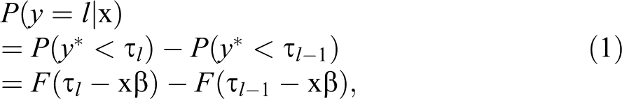
where
Other distribution functions are also possible, such as the probit (standard normal) or complementary log-log. Since the standard logistic distribution is the most widely used function for an ordered regression model, we focus on logit models in this article, but note that most of our discussions also pertain to models using alternative functions.
The parallel cumulative logit model is also known as the proportional odds model because if we have two x vectors, x1 and x2, then the two odds ratios,

based on equations (1) and (2) (McCullagh and Nelder 1989). In equation (3),
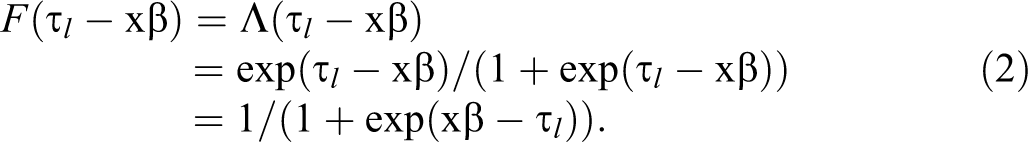
Ordered regression models with the parallel line assumption.
The parallel cumulative logit regression provides a parsimonious model for ordered responses. The PL assumption, however, that underlies the parallel cumulative logit model is a strong but hardly realistic assumption and thus is often violated in practice. The PL assumption is typically tested one coefficient or a subset of coefficients (e.g., a group of dummy variables for nominal-level variables) at a time, or for all coefficients simultaneously (i.e., omnibus test), and has the null hypothesis, H0:
Nonparallel and Partial Cumulative Logit Models
When the PL assumption is violated, researchers may turn to the nonparallel cumulative ordered regression model (also known as the generalized ordered logit model). Instead of having the same set of coefficients across cut-point equations, the nonparallel cumulative ordered regression model allows the coefficients to vary freely. In place of equation (1), we have

where
The partial cumulative logit model compromises between the parallel and nonparallel models by setting some of the coefficients to vary across equations and others to remain constant (see Fullerton [2009] and Fullerton and Xu [2016] for additional alternative model specifications). The model is given by:

where
Testing the Parallel Lines Assumption
A number of statistical tests have been developed to test the PL assumption. The most well-known include the Brant, Wald, likelihood ratio (LR), and score (or Rao or Lagrange multiplier) tests (Brant 1990; Buse 1982; Engle 1984; Fullerton and Xu 2016; Greene and Hensher 2012; Long 1997; Powers and Xie 2009). To summarize, the Wald test compares parameter estimates from the full model with those from a restricted (null) one normalized by standard errors of the estimates from the full. For a set of constraints imposed on the parameter estimates, such as

where
The LR test, on the other hand, compares the log-likelihoods from the full and restricted models. The test statistic has the following form

where
The score test is based on the gradient of the log-likelihood function of the restricted model normalized by its variance, and the test statistic is constructed as:

where
In this context, the full model may correspond to the nonparallel cumulative logit model in which the PL assumption is relaxed for all predictors, and a restricted model could refer to any reduced rank of the full model, such as a partial or a parallel cumulative logit model where the PL assumption holds for some or all predictors. Although all of the three tests are thought to be asymptotically equivalent, test results can diverge and have somewhat different properties in finite samples (see Fullerton and Xu 2016:132, for additional details and a comparison of the tests).
In addition to these classical null hypothesis significance testing (NHST) procedures, it is possible to compare the fit of models that maintain, relax, or partially relax the PL assumption using an array of R 2 measures (e.g., McFadden’s pseudo R 2, count R 2, and Lacy’s R 2) or model selection criteria (e.g., the Akaike information criterion [AIC] or the Bayesian information criterion [BIC]; Akaike 1974; Fullerton and Xu 2016; Greene and Hensher 2012; Lacy 2006; McFadden 1973; Raftery 1995; Schwarz 1978). In practice, however, given the lack of statistical distributions or agreement about which, if any, of the R 2 measures is best, researchers typically rely on one of the previously mentioned statistical tests for assessing the PL assumption.
Limitations with NHST of the PL Assumption
As Meehl (1967, 1997), Edwards and Berry (2010), and Kruschke (2017) cogently argue, the likelihood of rejecting null hypotheses in social sciences is generally high by design and they are often false a priori. When it comes to the PL assumption, first and foremost, the idea (or hypothesis) that the slopes for all predictors are equal across all cut-point equations is simply not realistic. In other words, it does not take a statistical test to realize that to satisfy all the conditions simultaneously is hardly possible. Second, if the coefficients for one or multiple predictors are statistically different based on an omnibus or semi-omnibus test, and we want to detect the exact source of that difference, we may have to conduct a series of tests or some form of simultaneous hypothesis testing; the former may increase the likelihood of a false alarm/positive, and the latter needs some form of adjustment/correction to be valid, which in many cases can be overly conservative (e.g., Bonferroni correction). Third, while testing the equivalence of two slopes across equations indexed by l and m for a predictor xk
, such as
Bayesian Approach to Cumulative Logit Models
A Bayesian approach to fitting cumulative logit models helps address some of the limitations of traditional methods to assess the PL assumption discussed previously. In this section, we specify the Bayesian parallel and nonparallel cumulative logit models, illustrate how to use both HDIs and ROPEs in evaluating the PL assumption, and propose a new Bayesian cumulative logit model with hyperparameters that provides an alternative approach to addressing variation in the coefficients across cut-point equations.
The fundamental equation within a Bayesian framework is given by:

where
A Bayesian parallel cumulative logit model can be specified as follows. First the likelihood conditional on the model parameters is given by:

in which
As usual, the posterior distribution of the model parameters is given by:

where

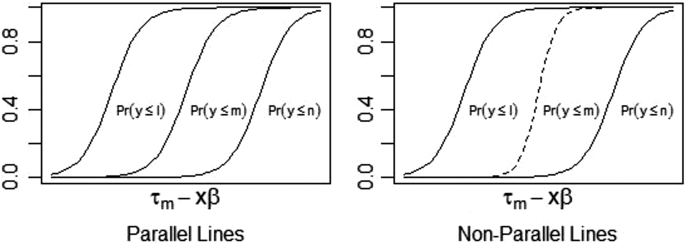
and the prior distributions for

with everything else stays the same as they are in the parallel cumulative logit model.
As discussed in Fullerton and Xu (2016), there are multiple ways to test the PL assumption in ordered regression models within a Bayesian framework. One method is to examine central intervals of the posterior of our interested quantity (e.g., the difference in two coefficients), for example, the 95 percent credible interval. With that, one simply finds the upper and lower bounds of the middle 95 percent of the posterior distribution with the two tails being equal. Based on decision theory, a better alternative is to find the middle 95 percent of the posterior that has densities higher than those outside the interval, hence the highest density interval (HDI) (Kruschke 2015; O’Hagan 2010).
As argued in the previous section, it is unlikely that differences in coefficients across cut-point equations will be exactly zero even in theory, and thus it is common to reject the PL assumption for even minor deviations given sufficient amount of data. One approach to address this issue is to allow for small differences in coefficients by defining a region of practical equivalence (ROPE) interval instead of point estimate for a Bayesian assessment of the PL assumption (Kruschke 2015; Kruschke and Liddell 2017). It can partly address the few problems associated with NHST and largely alleviate the problem of having inflated false positives arising from simultaneous and/or sequential testing of the PL assumption (Kruschke 2015; Kruschke and Liddell 2017). Instead of asking whether a significant mass of posterior distribution contains the null value (e.g., zero), the ROPE + HDI approach uses an interval, for example, [−0.5, 0.5], which could come from some scholarly consensus and be practically viewed as equivalent of the parameter value, usually 0, specified in the null.
Based on Kruschke (2015, 2017) and his colleagues (Carlin and Louis 2009; Hobbs and Carlin 2008), if the HDI (usually 95 percent HDI), the most representative range of the posterior, has no overlap whatsoever with the chosen ROPE for a parameter value, then the null hypothesis can be readily rejected; that is, the parameter value is not credible. If the HDI, however, falls completely within the ROPE, then the null value can be accepted, whereas under the frequentist framework, one can only fail to reject the null. When there is some overlap between the ROPE and the HDI, then one has to withhold the decision since there is not enough empirical evidence. The choice of the radius of a ROPE, of course, can affect the Bayesian assessment of null values. In some cases, prior scholarship may provide guidelines about an appropriate interval for the ROPE. In the absence of such guidelines, there are two recommended methods to define the ROPE interval. One is to examine the proportion (area) overlap between posterior and ROPE as a function of the radius chosen for ROPE so as to make this decision process open and transparent (Kruschke and Liddell 2017). A second method, again suggested by Kruschke (2015), is to set the ROPE interval to be
Note that while the ROPE + HDI method alleviates some of the problems previously described, it still stays within the conceptual framework under which coefficients are generally viewed as equal or unequal across equations. Next, we move beyond such conceptual limits to postulate that coefficients across different equations are allowed to be different to begin with, but since the data generation processes are usually presumed to be quite similar across different cut-points equations for the cumulative logit model, we also propose to maintain a higher order degree of homogeneity in that variation.
Hyperparameter Cumulative Logit Model
Considerable efforts have been made to adjudicate among parallel, partial, and nonparallel models (Fullerton and Xu 2016; Williams 2006). The parallel model has a clear advantage in parsimony, whereas the nonparallel model usually provides flexibility in parameterization, may increase predictive accuracy, and can accommodate nominality as opposed to strict ordinality of response variables. There are also other lesser known types, such as partial models, proportionality constraints, and stereotype models (Fullerton and Xu 2016, 2018). Despite the variety of these models, methods to select among them generally stay within the traditional NHST paradigm. Coefficients for the same predictors are either statistically not different from one another or they are different. In addition, existing literature does not distinguish between empirical and statistical significance; that is, two coefficients could be statistically different from one another, but they may produce trivial difference in predictions.
Because the likelihood of all coefficients for the same predictors being equivalent across the board is usually rather low especially given a large sample size, an omnibus test of the null hypothesis is often rejected. Conversely, allowing coefficients to vary freely across cut-point equations creates inefficiency and uncertainty about the ordinality of response variables. A common practice is then to let the data inform analysts by testing the PL assumption in an omnibus and then a pairwise (sometimes stepwise) manner, the latter of which can potentially compromise the power of the test (Gelman et al. 2012). Even with the Bayesian assessment of the PL assumption introduced in the previous section, some typical issues (e.g., allowing some coefficients to be different in certain way but not others) described here remain unresolved.
In this article, we propose a new cumulative logit model, in which its coefficients across cut-point equations do not have to be completely different, nor do they have to be exactly the same in the population. Instead, they are allowed to share the same population mean and variance (hyperparameters). This parameterization addresses several challenges that are usually associated with the traditional NHST framework, both conceptually and empirically. First and foremost, this new model recognizes that the PL assumption is simply unrealistic and this view is incorporated into the model setup. This model also acknowledges that there may exist some similarities across different pairs of logit comparisons; that is, the coefficients do not have to be drastically different given the ordinal, as opposed to nominal, nature of response variables and possibly follow similar data generation processes.
So the second approach we outline is the specification of a Bayesian cumulative logit model with hyperparameters that allow for the parameters of the same predictors to come out of the same distributions. This approach permits a degree of variation in the coefficients across cut-point equations but circumscribes these coefficients to share the same mean and variance. Similar to the shrinkage estimators in a multilevel model that uses partial pooling to weigh and thereby improve upon two classical estimates (i.e., no pooling and complete pooling), this hyperparameter cumulative logit model represents a synthesis of a nonparallel model that allows coefficients for each predictor to vary across all pairs of cut-point equations and a parallel model that imposes the restriction that the coefficients are equal across cut-point equations. Conceptually, this new model uses information from all cut-point equations for the same predictors to inform the estimation of specific coefficients so that parameter estimates are pulled toward the shared mean of the coefficient distributions. This is particularly useful when part of the model is unstable or even nonestimable as other parts of the model (i.e., data used to estimate other coefficients of the same predictors) can facilitate the estimation. In addition, this model simultaneously estimates cut points, coefficients, and their hyperparameters, all of which can be used for post-estimation analyses, interpretations, and predictions.
The Bayesian hyperparameter nonparallel cumulative logit model builds on the Bayesian nonparallel cumulative logit model specified previously in equations (13) and (14) by postulating the distributions for the coefficients as coming from same distributions (e.g., normal) with unknown means and variances (hyperparameters) and then specifying hyper-priors for these hyperparameters. For this new model, equation (14) is modified as follows,

and then hyper-priors are added to the model:

with the mean of coefficients following a normal, and the standard deviation following a Gamma distribution, and their corresponding hyper-priors are given in the parentheses.
Empirical Examples
The first empirical example examines sociodemographic predictors of self-rated health using data from the 2012 General Social Survey (Smith et al. 2019). Self-rated health is measured on an ordinal scale from one to four, denoting excellent, good, fair, and poor health, respectively. Predictors include age (in years), gender (male = 1 and female = 0), marital status (married = 1 and otherwise = 0), race (black and other race/ethnicity with white as the reference category), education (in years), and imputed log of family income. We use list-wise deletion to deal with missing data, which results in an estimation sample of 1,300.
For this example we use Stan Version 2.9 with the No-U-Turn Sampler (or NUTS) that optimizes Hamilton Monte Carlo adaptively to simulate the posterior (Carpenter et al. 2017; Gelman et al. 2014; Stan Development Team 2017). The tune, warm-up, and saved step sizes are set to be 2,000, 5,000, and 10,000, respectively, and three chains are used (Gelman et al. 2014; Hoffman and Gelman 2014; Kruschke 2015).
Table 1 reports descriptive statistics and estimates from both a standard parallel cumulative logit model (panel 1) and a Bayesian parallel cumulative logit model (panel 2) predicting self-rated health. Consistent with theoretical expectations, we see that age is associated with worse health, while education, income, and being married are associated with better health. We also note that the Bayesian model returns estimates of the parameters quite similar to those from the standard parallel cumulative logit model, except that the cut points are shifted parallelly due to the demeaned income in the Bayesian model for illustrative purposes.
Parallel Cumulative Logit Regression of Self-reported Health.
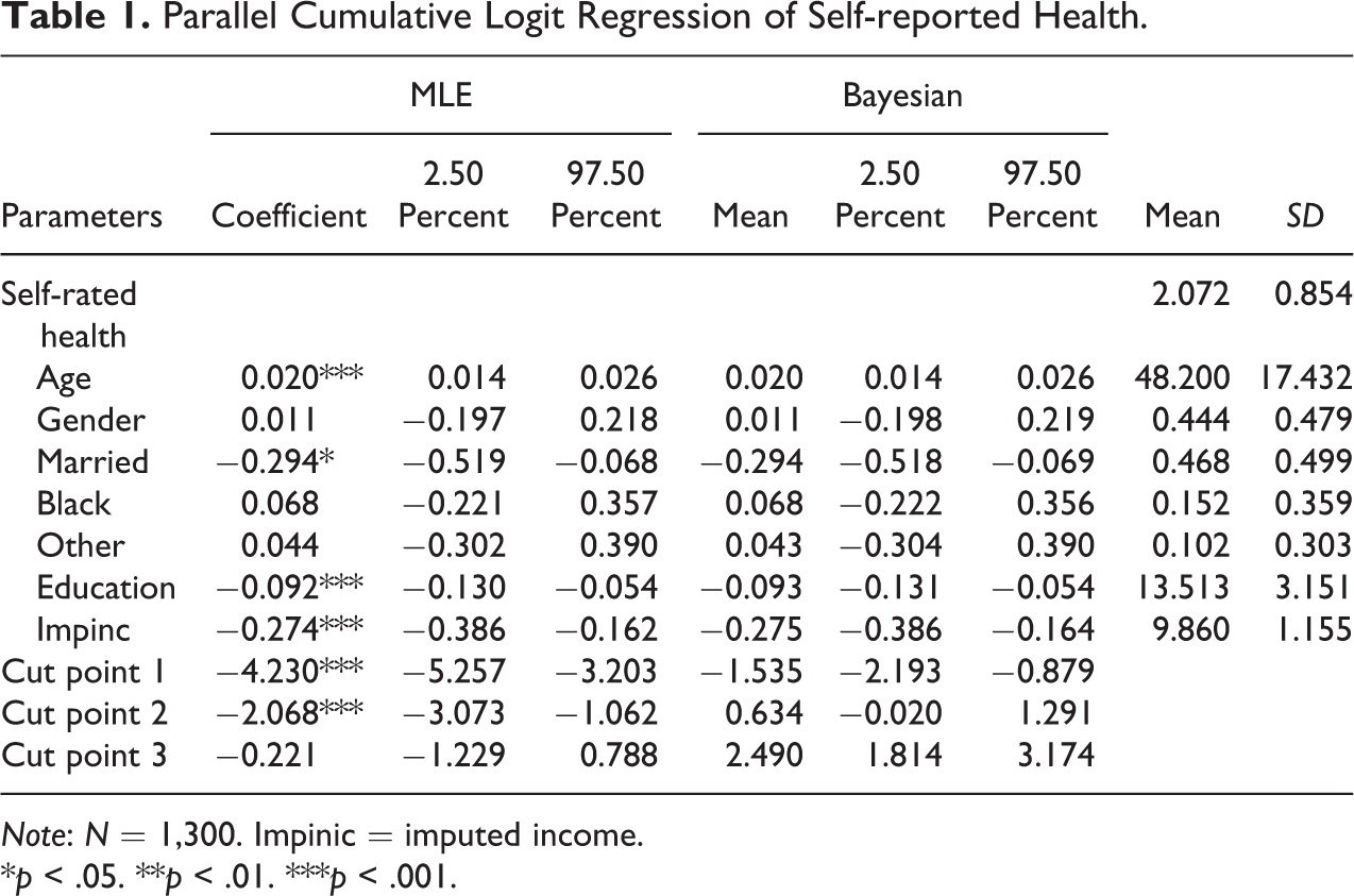
Note: N = 1,300. Impinic = imputed income.
*p < .05. **p < .01. ***p < .001.
Online Appendix 1-A (which can be found at http://smr.sagepub.com/supplemental/) reports various omnibus tests of the PL assumption for all predictors. All tests indicate that the PL assumption is violated for at least one of the predictors. Results from individual Brant tests (Online Appendix 1-B, which can be found at http://smr.sagepub.com/supplemental/) show that education and the black binary indicator of race fail to satisfy the PL assumption.
To further examine the source of the violation, we focus on testing the PL assumption for the coefficients of black and education. We first run a nonparallel cumulative logit model and then use this model as our baseline to conduct NHST (except when we run the Brant test using the parallel model). The left panel of Table 2 contains results from running a nonparallel cumulative model, and the results for testing the PL assumption for black and education are in Online Appendices 1-C, D, and E (which can be found at http://smr.sagepub.com/supplemental/). For both variables, we first examine whether their coefficients across cut-point equations are different in a pairwise manner and then in tandem with one another. With the significance level set to the traditional 0.05 level, the results for education are consistent across different tests that there is a clear violation of the PL assumption, but there exists some discrepancy as regards the black indicator variable. When we compare the black coefficients from the second (excellent and good vs. fair and poor) and the third equations (excellent, good, and fair vs. poor), the Wald, LR, and score tests all agree that the coefficients are pairwise different, and they are also consistent with one another that the difference in the black coefficients between the first (excellent vs. the rest) and second (excellent and good vs. fair and poor) equations is not statistically significant. But when we test whether the black coefficients are equal to one another as a group, these three tests come out differently, with the score test rejecting, LR marginally not rejecting, and the Wald test not rejecting the PL assumption. This example showcases that results from the three tests in nonasymptotic cases may be contradictory to one another, and usually the score and especially the LR test appear to be more conservative than the Wald test as indicated by prior scholarship (Engle 1984; Fullerton and Xu 2016). While examining various model fit statistics in Online Appendix 1-F (which can be found at http://smr.sagepub.com/supplemental/), it is hardly convincing that one model is necessarily better than the other between the parallel and nonparallel cumulative logit models.
Nonparallel Cumulative Logit Regression of Self-reported Health.
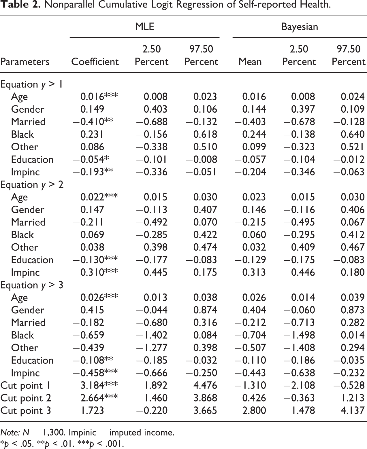
Note: N = 1,300. Impinic = imputed income.
*p < .05. **p < .01. ***p < .001.
The right panel of Table 2 reports the estimates from a Bayesian nonparallel cumulative logit model that serves as the basis for assessing the PL assumption. Again, it is not surprising that the estimates are quite similar to those produced by our ML estimation presented in the left panel of Table 2, given that weakly informative priors are used. To assess the PL assumption, we use both HDIs and ROPEs. While using some version of the credible interval (either central or highest density) alone, we simply look at whether the interval contains zero or not. For ROPEs, there are only some general guidelines for an assessment of null values as discussed in the previous section; to reiterate, if the ROPE we set for the parameter difference between two slopes is, for example, from −0.5 to 0.5 (i.e., a difference of 0.5 is not practically different from zero), and this region falls completely outside the 95 percent HDI, we can safely reject the null. If however the ROPE completely entails the 95 percent HDI, then we will accept the null. When there is just some overlap between the ROPE and HDI, we have to withhold our decision since there is not enough empirical evidence.
Figure 2 and 3 provide graphical displays of the results from our Bayesian inferential analysis of the PL assumption for the black and education coefficients, respectively. The left panel of both figures displays the posterior distribution and 95 percent HDI for a given ROPE radius, and the right panel graphs the proportion (area) of posterior within specified ROPEs as a function of the ROPE radius. Based on HDIs or simply credible intervals, the null value for two pairwise slope comparisons (the second and third graphs in Figure 2, that is, Eq1Black-Eq3Black and Eq2Black-Eq3Black) can be rejected since zero is outside the 95 percent HDI. But this conclusion can be misleading or premature because of, for example, the inconsistency between statistical and empirical significance or can be insufficient since sometimes we want to know whether we can accept the null value. Our following discussion focuses on left panels of the two figures first.
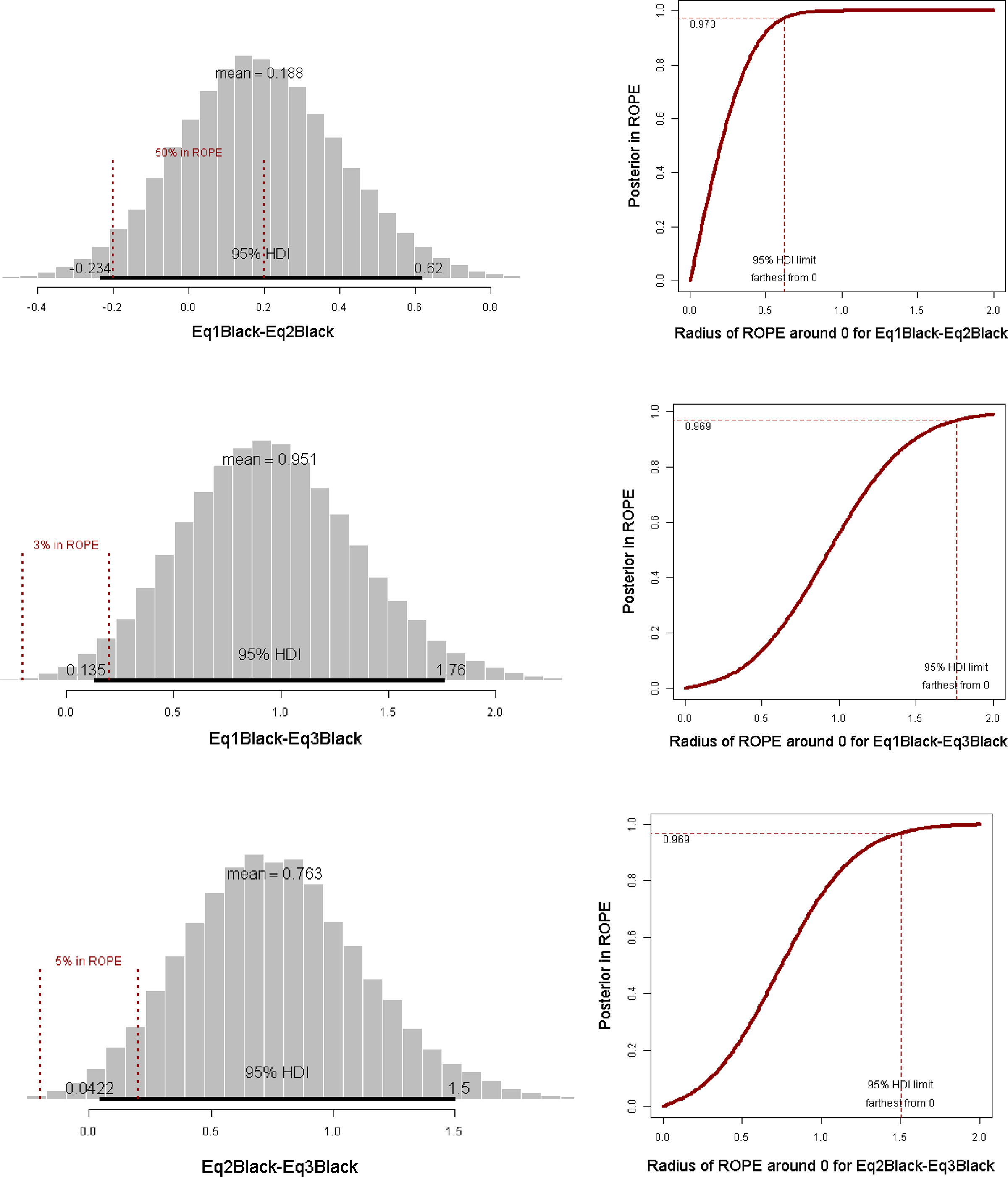
Testing black coefficients equivalence using regions of practical equivalence.
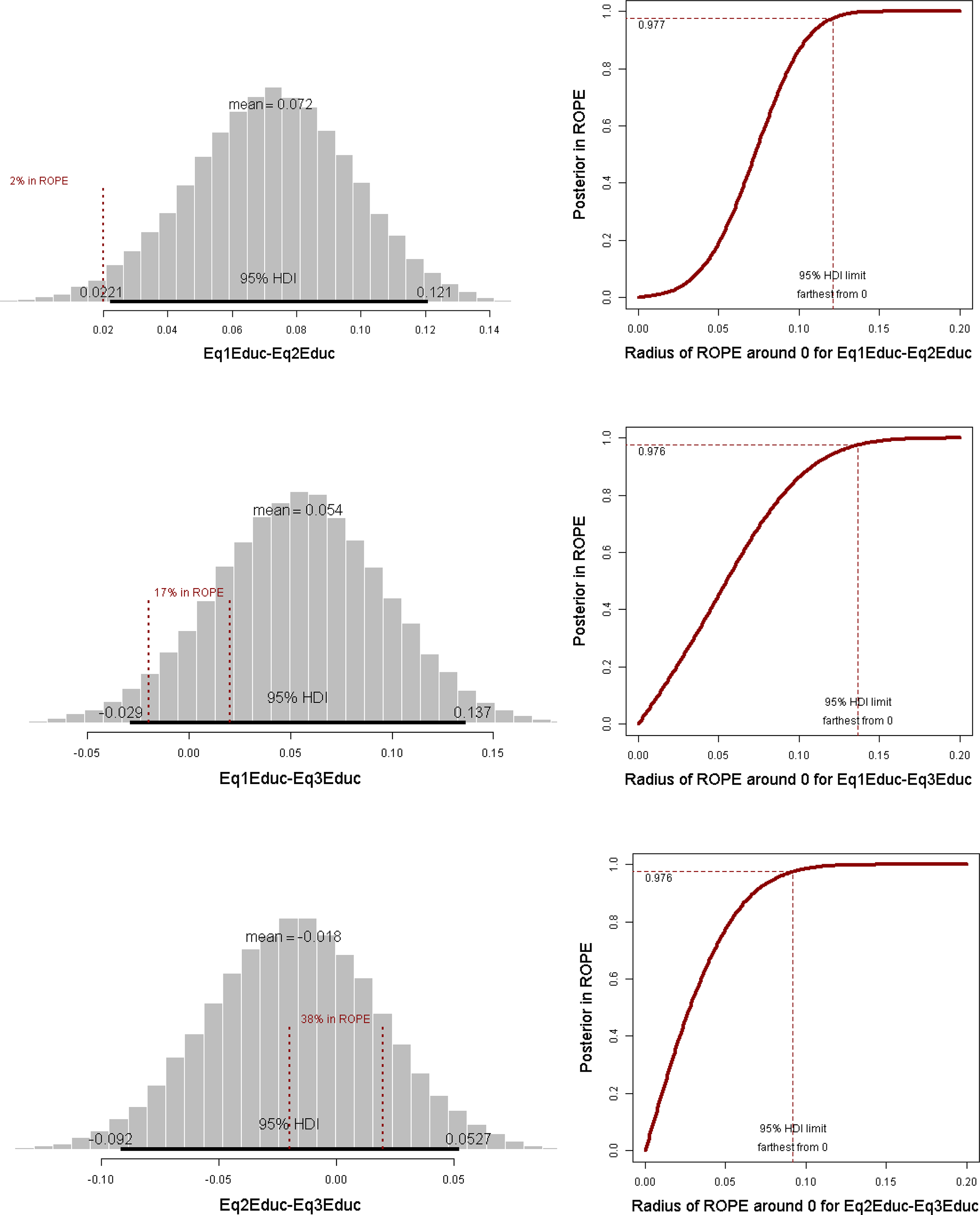
Testing education coefficients equivalence using regions of practical equivalence.
Following the
Similarly, Figure 3 provides a graphical display of the results from the Bayesian assessment of the PL assumption of the coefficients for education. Since it makes more sense to consider how ROPE is related to HDI in Bayesian inference, we focus on findings using a ROPE radius of 0.02. It can be shown that the two education slope parameters between the first and second equations are viewed as different since the 95 percent HDI is completely outside the specified ROPE. For the other two pairs of parameters, we have to suspend our judgment.
A different ROPE could, of course, lead to different conclusions concerning the validity of the PL assumption. For example, had we used a different ROPE radius, we would reject the null value about the difference between the black coefficients from the first and third equations (3 percent in ROPE with a radius of 0.2). Such a change would have to be more substantial in comparing the black coefficients between the second and the third equations (5 percent in ROPE with a radius of 0.2) and for the comparison between the first and second equations (50 percent in ROPE with a radius of 0.2).
To investigate how our results would vary with different ROPE radiuses, we also graph the proportion (area) of posterior within specified ROPEs as a function of the ROPE radius. These graphs are juxtaposed to the right of their corresponding graphs for (ROPE) radius-specific posterior distributions, and they in general agree with one another. If the curve (usually the low end) is steep, then that means the proportion of posterior in ROPE is quite sensitive to the chosen radius and accordingly it is less likely to reject the null. For example, although we probably have to withhold our decision as to our Bayesian assessment of the equivalence among the black coefficients given the chosen ROPE, we feel safer to infer that the black coefficients from the first and third equations (the second in the right panel of Figure 2) probabilistically bear less similarity than other pairwise comparisons since the amount of posterior in ROPE for the difference between the two coefficients stays low (<.05) before the radius hits 0.3, whereas the other two curves, especially the one for the comparison of the black coefficients between the first and second equations (the first in the right panel of Figure 2) goes up quickly, suggesting almost an infinitesimal likelihood that the ROPEd’ null value can be rejected. The pattern becomes even clearer in relative terms for the comparison of the two education coefficients between the first and second equations (the two graphs in the first row of Figure 3). Unlike the black–white decision rule under the NHST framework, the whole process of Bayesian assessment of null values recognizes uncertainty and is more transparent.
As illustrated, a Bayesian assessment of the PL assumption has a few advantages over the traditional frequentist NHST. First, it allows not only to reject but also accept the null. Second, it avoids the ambivalent and even confusing application of confidence intervals; instead, we can provide a full probabilistic interpretation of our results. Third, the use of ROPE + HDI reduces the odds of having false positives in sequential testing.
Estimation of the Hyperparameter Cumulative Logit Model
In this example, we use the same data from previous sections to fit a hyperparameter nonparallel cumulative logit model (see equation [15] and [16]). This model adds an additional assumption that slopes for the same predictors come from the same (normal) distributions. Table 3 presents Bayesian estimates of hyperparameters, means of slopes and cut points, and their 95 percent credible intervals from the posterior. Comparing the estimated means of slopes from the hyperparameter model with those from the parallel model, we find that both sets of coefficients are quite similar to the extent that all “statistically significant” coefficients are close to each other with regard to magnitude and exactly the same in direction. It is also of note that the mean estimates of statistically “credible” slopes and their credible intervals from the Bayesian hyperparameter nonparallel model (Table 3) are pooled closer to one another (hence the shrinkage estimators) than those from the Bayesian nonparallel model (Table 2) without hyperparameters or shrinkage.
Bayesian Hyperparameter Nonparallel Cumulative Logit Regression of Self-rated Health.
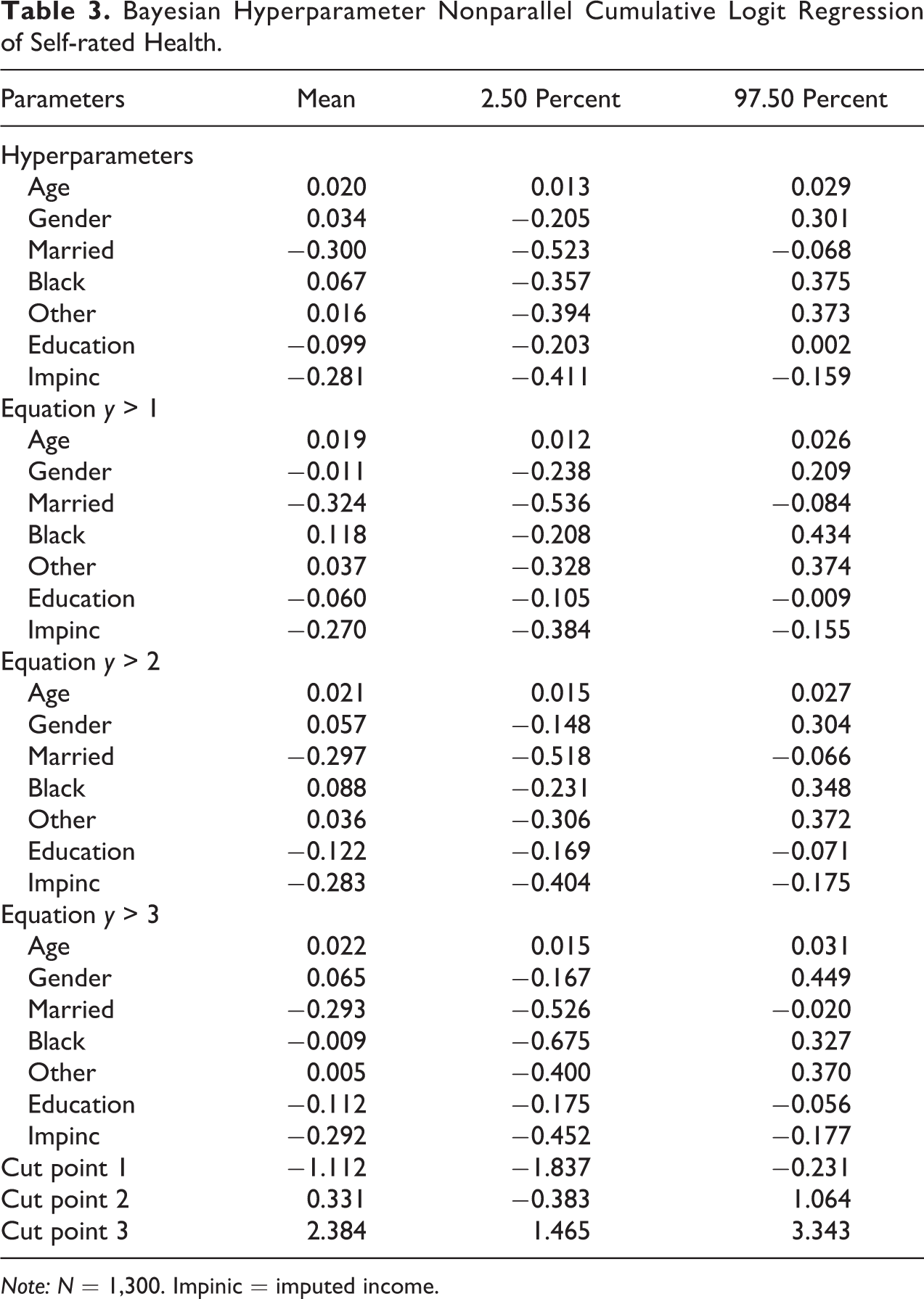
Note: N = 1,300. Impinic = imputed income.
Figures 4 and 5 plot predicted probabilities of y = 1, 2, 3, and 4 and their credible intervals from our estimation of the Bayesian parallel cumulative logit and the hyperparameter models, respectively. To compute these predictions and their credible intervals, we hold all other variables to their grand means while varying the values of log of family income. A few findings are worth noting. First, predictions across the two models are similar for one (y = 2) of the four response levels of self-rated health but are different for the other three. Second, the credible intervals for the hyperparameter model are clearly narrower than those of the parallel model for three of the four graphs (y =1, 3, and 4), indicating a superiority in precision.
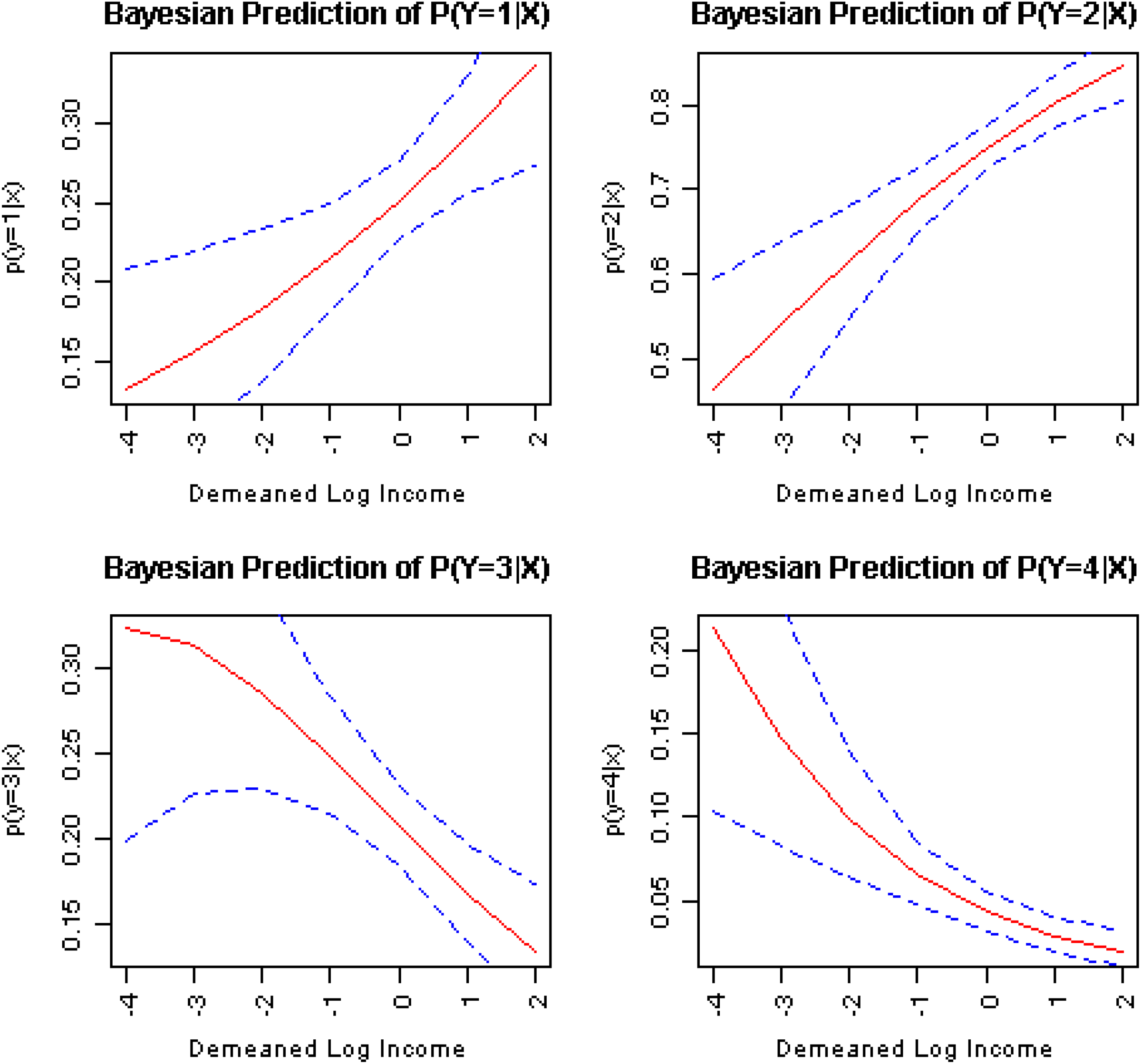
Predicted probabilities of four levels of self-rated health with credible intervals from the Bayesian nonparallel cumulative logit model.
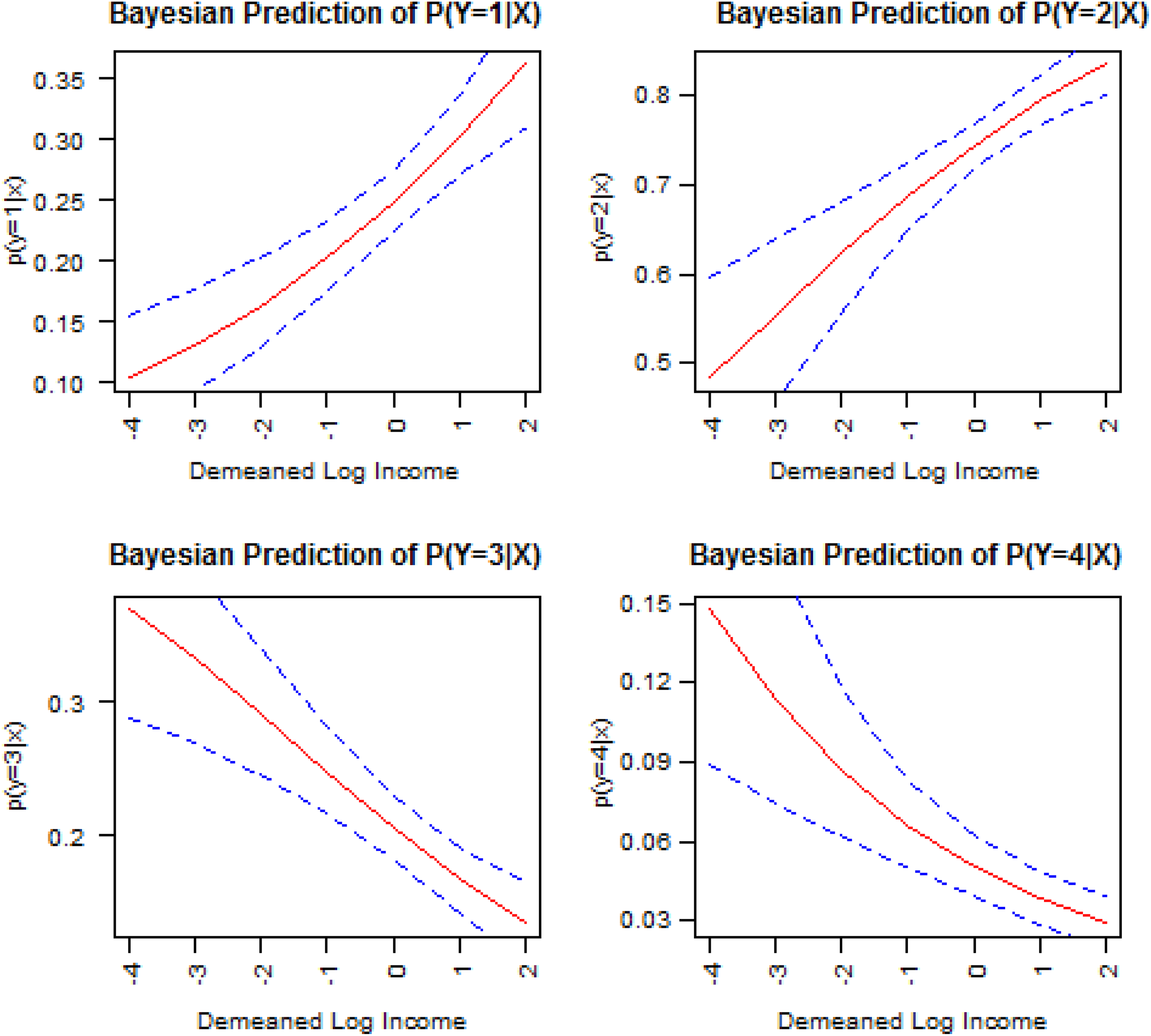
Predicted probabilities of four levels of self-rated health with credible intervals from the Bayesian hyperparameter nonparallel cumulative logit model.
Watanabe–Akaike (or more popularly, the widely applicable) information criterion (Vehtari, Gelman, and Gabry 2017; Watanabe 2010) is also used to evaluate and compare fitted Bayesian models. WAIC is calculated as

where
Second Empirical Example
In this second example, we use data from the Asian sample of the National Latino and Asian American Survey (Alegria et al. 2004) to illustrate how hyperparameter nonparallel cumulative logit model can be used where the traditional methods fail. In this example, we use an eight-level ordinal response to classify different types of body weight normalized by height based on standards set by the World Health Organization for body mass index (BMI). These eight levels include severe thinness (<16), moderate thinness (16–16.99), mild thinness (17–18.49), normal range (18.5–24.99), preobese (25–29.99), obese class I (30–34.99), obese class II (35–39.99), and obese class III (≥40). Age (in years), gender (male = 1), ethnicity (Filipino, Vietnamese, and other Asians with Chinese as the reference category), nativity (U.S. born = 1), marital status (married = 1), education (in years), and log of income (log of household income in dollars) are used as predictors. For this example, we first fit the traditional parallel cumulative logit model using maximum likelihood estimation (MLE), then the same model using Bayesian estimation, and last a Bayesian hyperparameter nonparallel cumulative logit model.
Table 4 presents results from the traditional frequentist parallel cumulative logit model using MLE. Age, being male vs. female, and being married vs. other types of marital status all increase the odds of having a heavier body weight adjusted by height. Being Filipino and other Asians as opposed to Chinese increase one’s odds of having a higher BMI type, whereas being Vietnamese vs. Chinese decreases the odds. Interestingly, both education and income are not associated with BMI types with desired significance level in this sample, though the signs of the coefficients are in expected direction. Not surprisingly, estimates from our Bayesian estimation of the same data and likelihood function with weakly informative priors yield very similar results.
Parallel Cumulative Logit Regression of Body Mass Index (BMI) Categories.
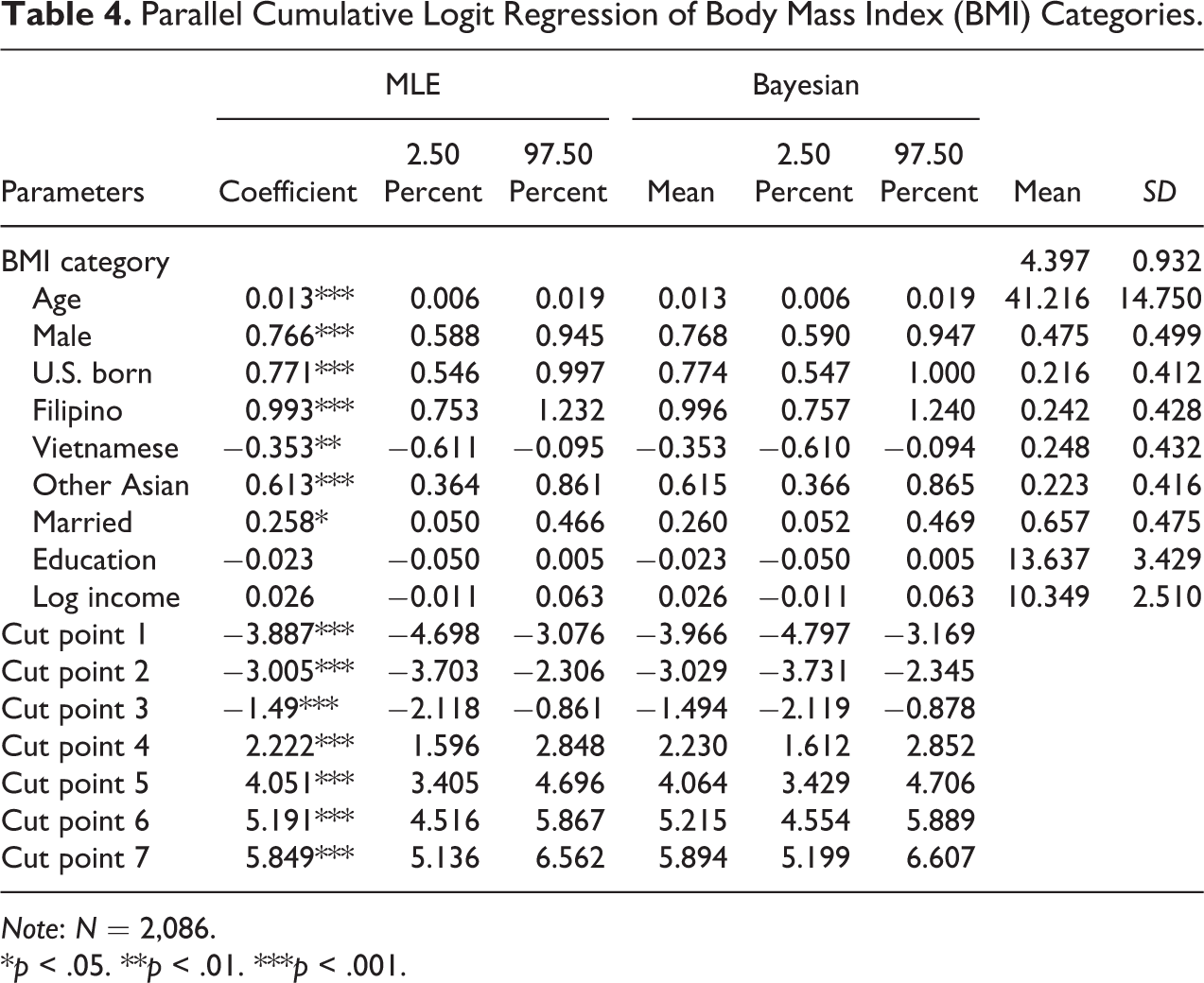
Note: N = 2,086.
*p < .05. **p < .01. ***p < .001.
While fitting a parallel cumulative logit model is not difficult, fitting a nonparallel cumulative logit model runs into numerical difficulties using either the MLE or Bayesian approach due in large part to the large number of response levels and the highly skewed distribution of the response variable. Therefore, a Bayesian hyperparameter nonparallel cumulative logit model (see equations [15] and [16]) becomes a natural candidate if we want to move beyond a simple parallel cumulative logit when a nonparallel model is not numerically estimable. Because fitting a Bayesian hyperparameter nonparallel cumulative logit model is computationally expensive, especially when we have an unusually large number of response levels, we need to revise a few initial MCMC simulation setups. We increase both the adapt and tune-in steps to be 5,000, with 285,000 steps (a total of 300,000 iterations) to be saved with three chains. Following Gelman (2006), we use the half-Cauchy distribution as priors for the scale hyperparameters of slopes in the model (see equation [16]), and results are presented in Table 5. 2
Bayesian Estimation of Hyperparameter Nonparallel Cumulative Logit Regression of Body Mass Index Categories.
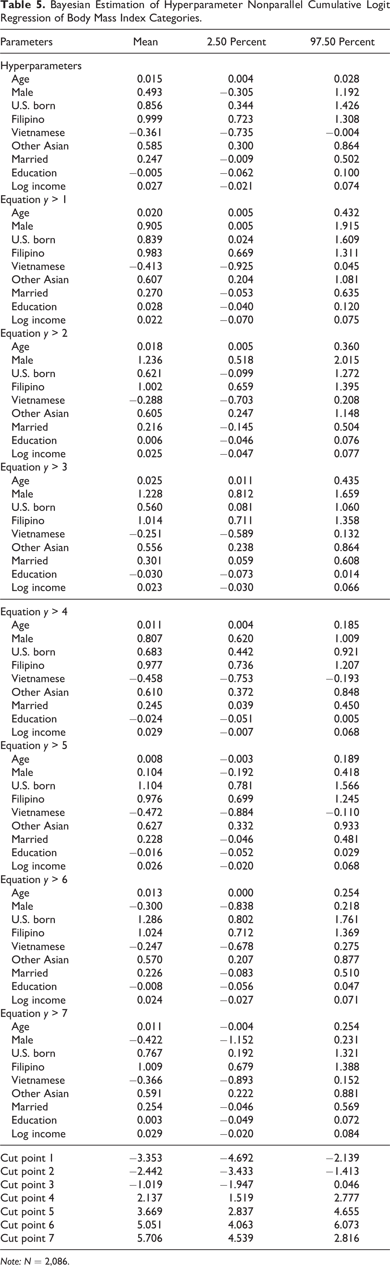
Note: N = 2,086.
The hyperparameter means of slopes from the hyperparameter model are similar to those from both the MLE and the Bayesian parallel model for some predictors but much less so for others; the estimates for Filipino, Vietnamese, other Asians, married, and log of income in three models are quite close to one another, somewhat different for age and U.S. born, and dissimilar for male and education. It happens that in this case, coefficients similar across models are all statistically significant, but for others that are dissimilar (i.e., male and education), they tend to be statistically insignificant across all models. Based on WAIC, it can be shown again that the Bayesian hyperparameter nonparallel cumulative logit model (WAIC = 4,559.8) clearly outperform the Bayesian parallel cumulative logit model (WAIC = 4,610.7). With estimates from the hyperparameter model, we can use hyperparameter means like we do in a parallel model to make predictions; alternatively, we could use estimate from those cut-point equations to conduct post-estimation analyses just like in a nonparallel model. We can even use some of the hyperparameter means for a subset of the predictors and estimates from cut-point equations for other variables, like in a partial model, for further analyses. This example clearly illustrates the utility of a hyperparameter model when the nonparallel model is numerically unestimable using either maximum likelihood or the Bayesian estimation method.
Practical Considerations
Despite several major advantages of using Bayesian estimation as illustrated in our article, there is one temporary limiting feature of this unorthodox statistical paradigm—computational cost. In this article, we ran three types of nonparallel Bayesian ordinal regression models using two different data sets. The amount of time required of such analyses depends on a few other factors than mere model complexity including sample size, adapt, burn-in, and final sampling steps. In addition, the elapsed time can vary drastically from chain to chain, especially with the MCMC used in Stan. When the results for this article were obtained, it took about one hour to estimates a Bayesian parallel cumulative logit model and three hours for the Bayesian nonparallel cumulative logit model, both with three chains, compared with a few seconds using the frequentist MLE, in a typical statistical environment (e.g., R, SAS, or Stata) on a typical personal computer (Intel i7-3770 CPU 3.4 GHz and 24 GB RAM). For the Bayesian hyperparameter nonparallel cumulative logit model, it took us about six hours to get convergence, and its frequentist counterpart is not yet available for estimation. There are various ways we can speed up the process, for example, using standardized variables and certain types of priors, such as half-Cauchy, for scale parameters. Given the high computational cost, Bayesian estimation of cumulative ordered logit is usually preferred when one intends to use informative priors and/or complex reparameterization. Of course, the concern about some fundamental flaws of NHST and an embrace of the whole new Bayesian inferential framework is another important consideration.
Conclusion
This article outlines Bayesian approaches to address several long-standing issues related to the PL assumption with ordered regression models. First, this article introduces a Bayesian assessment of null values as a useful alternative for testing the PL assumption. While the traditional NHST framework has reached a high level of sophistication, it suffers from several major limitations. First and foremost, testing the PL assumption under the NHST framework simply recreates part or whole of the Meehl’s paradox that the null here is inherently untenable; it is unrealistic in presuming that all slopes for the same predictors are exactly the same across different cup-point equations, and even a minor deviation may lead to the rejection of the PL assumption. Moreover, one may have to go through a stepwise procedure to find the source of violation of the PL assumption, which may compromise the power of the test and inflate false alarms. Third, the traditional NHST framework can only allow one to fail to reject but not to accept the null; last but not least, under the old paradigm, one can only calculate the probability of observing the data given the null is true, whereas what is often sought after is the probability that the null is true given the data. The use of Bayesian assessment of null values through HDIs + ROPEs can alleviate or avoid some of these problems.
A second major contribution of this article is to propose a Bayesian hyperparameter nonparallel cumulative logit model, providing a fresh new perspective on how to deal with possible violations of the PL assumption. Instead of having to choose between parallel and nonparallel slopes, or some partial version in between, this new model allows slopes to be somewhat different to the extent that their means come from the same distribution dominated by hyperparameters. Our empirical examples show promising results for this new model.
Supplemental Material
Supplemental Material, Supplemental_Material - Bayesian Approaches to Assessing the Parallel Lines Assumption in Cumulative Ordered Logit Models
Supplemental Material, Supplemental_Material for Bayesian Approaches to Assessing the Parallel Lines Assumption in Cumulative Ordered Logit Models by Jun Xu, Shawn G. Bauldry and Andrew S. Fullerton in Sociological Methods & Research
Footnotes
Authors’ Note
An earlier version of this article was presented at the 2017 ASA Methodology Midyear Meeting in Chicago. Usual disclaimers apply.
Declaration of Conflicting Interests
The author(s) declared no potential conflicts of interest with respect to the research, authorship, and/or publication of this article.
Funding
The author(s) received no financial support for the research, authorship, and/or publication of this article.
Supplemental Material
Supplementary material for this article is available online.
Notes
References
Supplementary Material
Please find the following supplemental material available below.
For Open Access articles published under a Creative Commons License, all supplemental material carries the same license as the article it is associated with.
For non-Open Access articles published, all supplemental material carries a non-exclusive license, and permission requests for re-use of supplemental material or any part of supplemental material shall be sent directly to the copyright owner as specified in the copyright notice associated with the article.