Linking Input Inequality and Outcome Inequality

Abstract

Inequality often appears in linked pairs of variables. Examples include schooling and income, income and consumption, and wealth and happiness. Consider the famous words of Veblen: “wealth confers honor.” Understanding inequality requires understanding input inequality, outcome inequality, and the relation between the two—in both inequality between persons and inequality between subgroups. This article contributes to the methodological toolkit for studying inequality by developing a framework that makes explicit both input inequality and outcome inequality and by addressing three main associated questions: (1) How do the mechanisms for generating and altering inequality differ across inputs and outcomes? (2) Which have more inequality—inputs or outcomes? (3) Under what conditions, and by what mechanisms, does input inequality affect outcome inequality? Results include the following: First, under specified conditions, distinctive mechanisms govern inequality in inputs and inequality in outcomes. Second, input inequality and outcome inequality can be the same or different; if different, whether inequality is greater among inputs or outcomes depends on the configuration of outcome function, types of inputs, distributional form of and inequality in cardinal inputs, and number of and associations among inputs. Third, the link between input inequality and outcome inequality is multiform; it can be nonexistent, linear, or nonlinear, and if nonlinear, it can be concave or convex. More deeply, this work signals the formidable empirical challenges in studying inequality, but also the fast growing toolbox. For example, even if the outcome distribution is difficult to derive, fundamental theorems on the variance make it possible to analyze the input–outcome inequality connection. Similarly, within specified distributions, the general inequality parameter makes it possible to express results in terms of both measures of overall inequality and measures of subgroup inequality.

Keywords

inputs outcomes input–outcome relations probability distributions inequality measures lognormal/Pareto/power-function/rectangular distributions Atkinson/Gini/Theil inequality measures new unified theory of sociobehavioral processes justice status power surprises

Introduction

Inequality is pervasive in the social life, and understanding inequality is a basic task for sociology. How and why the Weberian life chances differ across individuals, how the various inequalities are generated and eradicated, and how objective inequalities are transformed into subjective inequalities—these are matters that lie at the heart of the sociological project. Although much has been learned about the operation of inequality, much remains to be learned. In Darity and Deshpande’s (2000:77) words, the goal is to understand the “deep structure” of inequality.

This article expands the toolbox for studying inequality by introducing a methodological framework that begins with relations between inputs and outcomes and makes explicit the distinction and connection between inequality in inputs and inequality in outcomes. The motivating idea has been known for a long time. To illustrate, it is common to speak of “income,” “status,” and “how income generates status.” For example, Veblen ([1899] 1953) observes, “the possession of wealth confers honor.” Thus, there are inputs like income and outcomes like status that are generated by the inputs, and both inputs and outcomes can have their own magnitudes of inequality. Explicit attention to inputs and outcomes and their interconnections may shed light on some puzzles, for example, why economic equality is fragile, why some groups seem to have a low degree of experienced inequality even when their income inequality is high or why some groups have an unchanging degree of experienced inequality even when their income inequality changes.

Of course, a particular variable can appear in several ways in input–outcome relations. First, it can be an input in a single relation or in several relations. To illustrate the latter, income is an input to both status and self-esteem; similarly, cognitive skill is an input to both schooling and wage. Thus, a variable can be a popular input—or, as the saying goes, it can “dance at many weddings.”

Second, a variable can be the sole input to an outcome or it can share inputhood. Put differently, an outcome can be generated by more than one input simultaneously. For example, status can be generated jointly by both athletic skill and wealth; the link between inequality in athletic skill and inequality in status may differ from the link between wealth inequality and status inequality. In these multiple-input cases, it is useful to contrast the distributions of the inputs and the outcome as well as the inequality in the inputs and outcome. Early examples of the first include Quetelet’s ([1835] 1842) and Galton’s (1899) reasonings about the expected normality of human traits. The best early example of the second is Jencks et al.’s (1972:12, 352) discussion of the links between cognitive inequality, educational inequality, and economic inequality.

Third, a variable can be an outcome in one relation and an input in another. For example, income appears as outcome in the relation between schooling and income, and it appears as input in the relation between income and consumption as well as in the relation between income and status. Indeed, there can be long chains of variables in input–outcome relations, for example, cognitive skill to schooling to wage to status and so on. Variables with a dual input–outcome existence are exceptionally rich to study; clear understanding of their operation requires attention to whether, in a particular context, they are operating as an input or instead as an outcome.¹

But we are getting ahead of ourselves. We start simple. Methodologically, the key to the framework is the twofold idea (1) that there is a special relation between input and outcome and (2) that input and outcome each have a distribution. Thus, for example, if we know the special relation—the function connecting input and outcome—and if we know the distribution of the input, we can obtain the distribution of the outcome. And from the input distribution and the outcome distribution, we obtain the input inequality and the outcome inequality—and link them.

This article takes a modest step, and the goal of linking input inequality and outcome inequality will benefit from much further scrutiny, both theoretical and empirical. For now, we explore the general inequality connection across inputs and outcomes by addressing three main questions:

How do the mechanisms for generating and altering inequality differ across inputs and outcomes?

Which have more inequality—inputs or outcomes?

Under what conditions, and by what mechanisms, does input inequality affect outcome inequality?

To address these questions, we develop, in the second section, a general theoretical and methodological framework applicable to a wide range of inputs and outcomes, input–outcome relations, and distributional forms, and incorporating ideas, insights, and procedures from the literature, which together enable analysis of the inequality connection across inputs and outcomes.

But given the abundance of inputs, input–outcome functions, and input distributions, and for simplicity and concreteness, in this first presentation of the framework, we provide a theory-based application with a starter set of three input–outcome relations and four input distributions. As will be seen, these provide a clear view of procedures and of the remarkable diversity of connections between input inequality and outcome inequality.

The setup for the application is described in the third section. The input variables are positive variables; the three input–outcome relations are increasing functions. The three functions differ by whether the outcome increases at a decreasing rate or at an increasing rate or at a constant rate. The first two are nonlinear, the first concave downward, the second concave upward. The two nonlinear functions are theory-based specific functions; of course, there are many more nonlinear functions to be analyzed by future work originating in the general framework. The third function is linear, and results obtained in the application apply to all linear functions.

Given the focus on positive variables in the application, the modeling distributions for the input are defined on the positive support. Accordingly, we use the unit rectangular to model ordinal variables, and to model cardinal variables, we use three distributions that are widely used to model income and other size distributions and whose properties are well understood—the lognormal, Pareto, and power-function (Johnson, Kotz, and Balakrishnan 1994–1995; Kleiber and Kotz 2003).

The three main questions about input inequality, outcome inequality, and their link are addressed, for the theory-based application, in the fourth to sixth sections. The fourth section addresses the first question, contrasting the rules that govern inequality in inputs and outcomes and summarizing inequality measures. Next, in the fifth section, we compare inequality across inputs and outcomes. As will be seen, this contrast is straightforward in some cases, elaborate in others. There are at least two reasons why the outcome distributions may differ from the input distributions (leading to different inequality). First, except in some special cases (such as when the outcomes are identity functions of the inputs, i.e., Y = X), the outcome distributions will differ from the input distributions. Second, in the case of multiple inputs, the outcome distribution may differ from all the component input distributions. Finally, in the sixth section, we examine the effects of input inequality on outcome inequality. Along the way, we encounter three of the great surprises of theoretical analysis: (1) novel predictions in deductive theory (subsection on Connections Between Personal Attributes and Possessions and the Primordial Sociobehavioral Outcomes), which are a substantively special kind of input–outcome relations; (2) new probability distributions (subsection on Deriving the PSO Distribution in the Multiple-Good Case and subsection on Inequality Contrasts Involving the Two-Identical-Good Status PSO World), which are substantively special outcome distributions obtained by combining an input distribution with an input–outcome relation; and (3) theoretical unification (starting in the third section), exemplified in the new unified theory (NUT) which integrates three theories with a parallel structure in which each theory’s defining input–outcome relation has a distinctive rate of change. More deeply, the unified theory exemplifies a Mertonian middle-range theory—a step deeper than the three Mertonian middle-range theories it unifies. Overall, the work reported here illustrates the essential unity of the methods that advance both theoretical and empirical knowledge. A short note concludes.

General Theoretical and Methodological Framework

This section assembles the building blocks for linking input inequality and outcome inequality: the input variables, the functions linking inputs and outcomes, the modeling distributions for the inputs, procedures for deriving the outcome distributions, and measures of inequality. Thus, the stage is set for analyzing the connection between input inequality and outcome inequality in any application of interest.

Inputs

In general, the inputs are quantitative variables, denoted X. Quantitative variables refer to properties or features of which there can be “more” or “less”—more skill, less land, more war deaths, less parental involvement. Though the vocabulary and rubric may differ across disciplines, several major dimensions may be discerned. Quantitative variables can be cardinal (like wealth) or ordinal (like beauty). Quantitative variables can be continuous (like age and teacher advising time) or discrete (like number of children and war deaths). Quantitative variables may be represented by distinctive sets of numbers—defined, for example, as positive, nonnegative, negative, nonpositive, or spanning the full set of real numbers.²

Behaviorally, quantitative variables can be “goods,” if observers prefer more to less, or “bads,” if observers prefer less to more. Moreover, quantitative variables can be “earned” (like wages) or “unearned” (like windfalls). Finally, though inequality measures like the Gini coefficient can always be calculated in quantitative variables, “shares” are natural in cardinal things but not in ordinal things.³

Input–Outcome Relations

As with inputs, there is a wide variety of input–outcome relations, and a wide variety of dimensions for describing them. First is the number of inputs. Some outcomes depend on a single input, others on two inputs, still others on multiple inputs.⁴ Second, input–outcome relations can be monotonic or nonmonotonic. Third, if monotonic, they can be increasing or decreasing. Fourth, if nonmonotonic, they can display a variety of shapes, such as U-shape and inverted-U-shape. Fifth, functions can have distinctive rates of change, their graphs bending upward or downward, over the whole curve or over distinct regions.

Concomitantly, input–outcome relations can be deterministic or stochastic. Prominent examples of deterministic relations include identities such as the national income equation (consumption plus investment), couple’s combined income (wife’s income plus husband’s income), business net income (revenues minus expenses), and personal posttax income (pretax income minus taxes). Importantly, identities can be useful for estimating stochastic relations, as in the textbook example from Keynesian economics, where the national income identity is used to overcome the biasing effects of income endogeneity in the consumption function and obtain a consistent estimate of the effect of income on consumption (Ashenfelter, Levine, and Zimmerman 2003:220-27; Wonnacott and Wonnacott 1979:257-65). While deterministic equations have no parameters and no error term, stochastic equations have both. Thus, the two kinds are easy to spot visually.⁵

Table 1 reports a variety of examples of input–outcome relations, classified into three sets. The first set includes two-input relations in which the outcome is the sum of the two inputs; the second set includes two-input relations in which the outcome is the difference between two inputs; and the third set includes multiple-input relations.

Table 1.

Inputs and Outcomes in Two-Input and Multiple-Input Relations, Classified by the General Form of the Input–Outcome Relation.

1. $Y = X_{1} + X_{2}$
Outcome Y	Input X₁	Input X₂
Child well-being	Father involvement	Mother involvement
Student performance	School resources	Home resources
Worker performance	Cognitive skills	Noncognitive skills
Couple’s combined income	Husband’s income	Wife’s income
Income	Earned income	Unearned income
2. $Y = X_{1} - X_{2}$
Outcome Y	Input X₁	Input X₂
Spouses’ income disparity	Husband’s income	Wife’s income
Marital cohesiveness	ln(husband’s income)	ln(wife’s income)
Posttax income	Pretax income	Tax
Justice evaluation	ln(actual reward)	ln(just reward)
Change in well-being	Income at Time 1	Income at Time 2
3. $Y = \sum X_{i}$
Outcome Y	Inputs X_i
Child well-being	Home, school, and extracurricular activities
Educational attainment	Cognitive skills, noncognitive skills, and school resources
ln(Wage)	Schooling, experience, performance, and noncognitive skills
Wage	Wages recommended by wage-setters
Multi-good justice evaluation	Single-good justice evaluations
Multi-good status	Single-good status scores

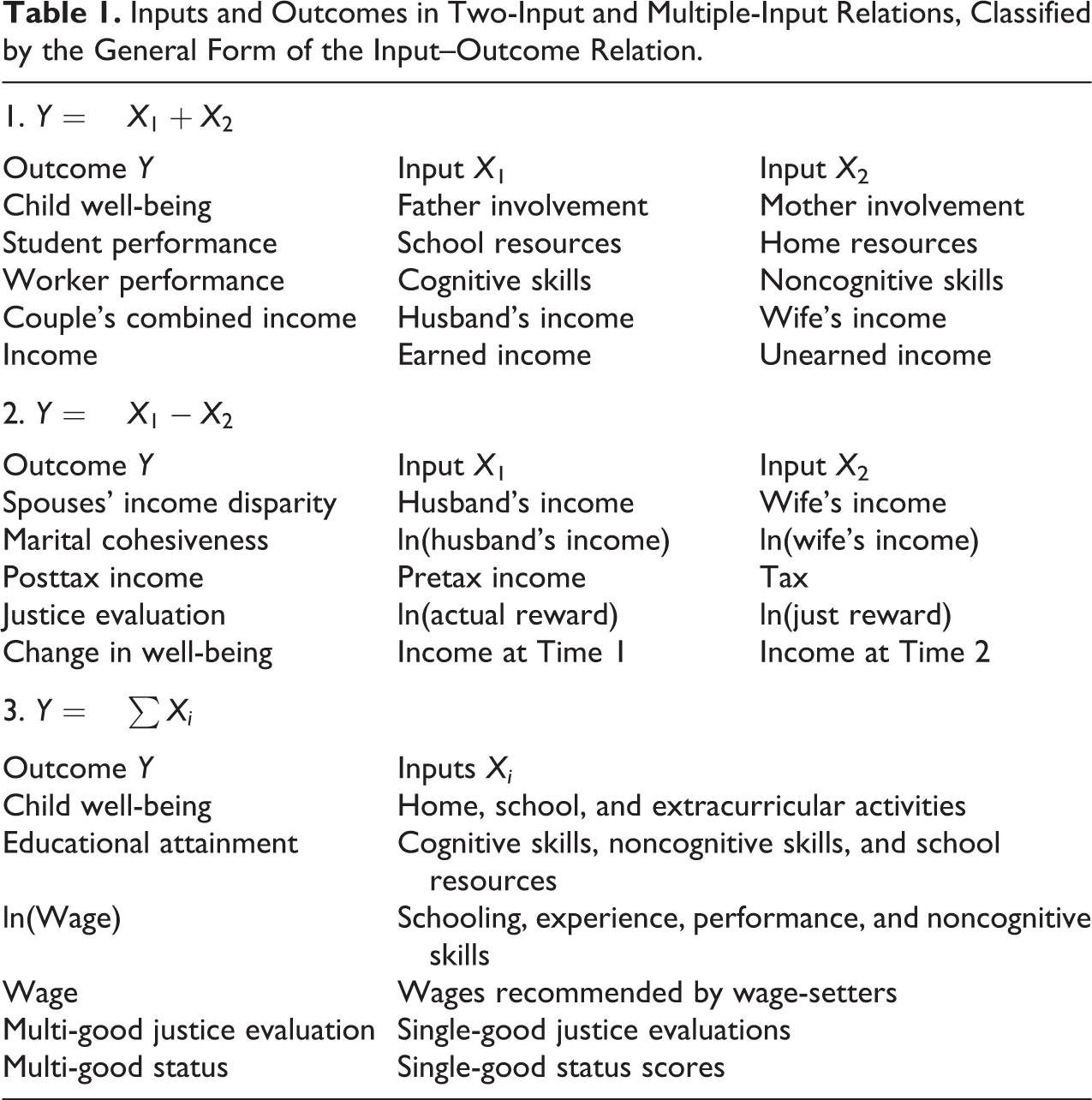
The reader will recognize that some of the input–outcome relations in the table require parameters and others not. To illustrate, couple’s combined income and spouses’ income disparity would not have parameters. In contrast, the student performance relation would have parameters. And in the relation specifying a person’s wage as the average of the wage amounts recommended by a group of wage-setters, the parameters are weights which sum to 1.

The reader will also recognize that although all the relations in Table 1 are expressed as sums or differences, some of the underlying relations are multiplicative—marital cohesiveness and the justice evaluation in panel 2 and the ln(wage) function in panel 3.

Selecting the Modeling Distributions for the Inputs

The key underlying idea is that if we know the probability distribution of the input X and we know the function that connects X to the outcome, we can derive the distribution of the outcome—and proceed to analyze inequality in the distributions of both input and outcome. Selecting modeling distributions for the inputs is thus an exercise in matching the characteristics of the input (e.g., the region of the number line used to represent it and whether it is continuous or discrete) to available mathematically specified distributions.

Collections of distributions include the introductory Gallery of Distributions in the online eHandbook of Statistical Methods (also known as the Engineering Statistics Handbook) published by the U.S. National Institute of Standards and Technology (2018), the one-volume Forbes et al. (2011), and the comprehensive compendia originated by Johnson and Kotz (1969–1972) and continued with Balakrishnan and Kemp (e.g., Johnson et al. 1994–1995; Johnson, Kemp, and Kotz 2005). Briefer introduction is provided in Jasso and Liao (2003) and Jasso and Kotz (2008a).

When the input X is perfectly equally distributed, the equal distribution (sometimes called “degenerate” when defined as discrete, and “Dirac’s delta” when defined as continuous) provides a model for a perfectly equal distribution and thus serves as a benchmark in studies of inequality.

For nonequal discrete variables, modeling distributions include the binomial, the hypergeometric, and the Poisson.

Ordinal inputs are represented by the set of relative ranks and thus modeled by the (continuous) unit rectangular distribution.

For nonequal continuous Xs spanning the full set of real numbers, some useful modeling distributions include the normal, Cauchy, logistic, Laplace, and extreme value distributions.

For nonequal continuous Xs defined on the positive support, a useful set of modeling distributions includes the lognormal, Pareto, and power-function. The lognormal is defined for all positive values, the Pareto for all positive numbers larger than a specified number, and the power-function for all positive values smaller than a specified number. Thus, the Pareto can be used for modeling situations with a minimum income and the power-function for situations with a maximum income (whether due to natural scarcity or a social rule, as in Plato ([c.428-348/7 BC] 1952), Laws V).

Formulas and graphs for the main associated functions of these variates—the probability density function (PDF), the cumulative distribution function (CDF), and the quantile function (QF)—are widely available.⁶

Tools for Finding the Distribution of a Function of One or More Variables

Distribution of a function of one variable

The problem of finding the distribution of a function of one variable is usually stated in the form: Given the function y = h(x) and given the distribution of X, what is the distribution of Y? The best-known procedure is the change-of-variable technique based on the PDF (Hoel 1971:244-48). An alternative and extremely simple procedure is based on the QF; this procedure can be used whenever the QF of X has a closed-form expression, as in the Pareto and power-function variates, or can at least be written down, as in the lognormal.⁷

Distribution of a function of several variables

Following the literature, a starting approach in this more elaborate situation in which Y is a function of several Xs is to define six special cases, obtained by crossing two dimensions: (1) whether the X distributions are identical or different; and (2) whether the X distributions are independent, perfectly positively associated, or perfectly negatively associated (with negative association given a special meaning in the case of three or more Xs).

Perfect positive association denotes the case in which each person (or, more generally, unit) has the same relative rank on all the Xs. Independence denotes the case in which the X distributions are statistically independent. Perfect negative association denotes, when the number of Xs is two, the case in which the rank ordering of one of the Xs is exactly the reverse of the rank ordering of the other X. When the number of Xs exceeds two, we use the method of organized subsets introduced by Berger et al. (1977), such that within each subset, all the Xs are perfectly positively associated and the two subsets are perfectly negatively associated. Of the six special cases, the combination of identical and independent is the most familiar, as many statistical results used in empirical social science are based on identical and independently distributed variables—the iid case. The six cases may be considered ideal types, covering possibilities for a broad range of social, economic, and political circumstances.

Measures of Inequality

The goal is to contrast and link input inequality and outcome inequality. Accordingly, the set of inequality measures to be used must reflect two considerations. First, it must include both measures of overall inequality and measures of subgroup inequality. Second, it must include measures for variables defined on any region of the real line.

Overall inequality refers to inequality between persons (or units, more broadly), while subgroup inequality refers to inequality between subgroups (Jasso and Kotz 2008b). Overall inequality is measured by the classic measures such as the Gini (1914) coefficient, the Atkinson (1970) measure defined as one minus the ratio of the geometric mean to the arithmetic mean, the two Theil (1967) measures (Theil Index and Theil MLD), and the coefficient of variation. Subgroup inequality, in the case of two subgroups (or within a pair of subgroups), is measured in two main ways, by the ratio of the mean in one subgroup to the mean in the other subgroup and by the absolute difference between the means of the two subgroups. Formulas for both overall and subgroup inequality measures, for both observed and mathematically specified distributions, are widely available (e.g., Jasso and Kotz 2008b:38-39, 45; Jasso 2018:201). Note that the Atkinson measure used here and the Theil MLD both depend on ratios of the geometric mean and the arithmetic mean and are thus transformations of each other (Cowell 2011:186).

In a subset of mathematically specified distributions, namely, continuous univariate two-parameter distributions, the second (nonlocation) parameter operates as a general inequality parameter, denoted c, which governs all measures of inequality (Cowell 1977:95; Cramer 1971:51-58; Jasso and Kotz 2008b:35-49; Kleiber and Kotz 2003:78). Measures of overall inequality are functions only of c, and they are monotonic functions of c; measures of subgroup inequality are also monotonic functions of c, but c is not the only parameter on which they depend. Ratio measures of subgroup inequality depend as well on the percent split, represented by the proportion in the bottom subgroup p, and difference measures of subgroup inequality depend not only on c and p but also on the overall mean μ (Jasso 2020:967-68; Jasso and Kotz 2008b:44-46).

As for the second consideration, we distinguish between variables defined on the positive segment and variables that include as well zero and negative values. Positive variables are compatible with all the measures of inequality. However, for variables spanning positive and negative values, applicable measures are a smaller subset, including the Gini’s mean difference (GMD) and the variance to measure overall inequality and the difference-based measure of subgroup inequality.⁸

Finally, a threefold practical note. First, because the general inequality parameter c governs all inequality measures in continuous univariate two-parameter distributions, theoretical results can be obtained for such distributions even if it is difficult to obtain expressions for specific measures (such as the Gini coefficient or Atkinson inequality). Second, because overall inequality and subgroup inequality are both monotonic functions of c, results for measures of overall inequality in continuous univariate two-parameter distributions imply results for subgroup inequality. Third, even if the distributional form for the outcome is difficult to derive, it will still be possible to work with its variance—given the arsenal of useful theorems on the variance—and thus analyze the connection between input inequality and outcome inequality.

Special Setup for Theory-based Application: The NUT and Its Two Worlds of Inequality

The general framework is of broad applicability, comprising diverse kinds of inputs and outcomes and diverse kinds of input–outcome relations. To illustrate the framework, we examine the connection between input inequality and outcome inequality in a special theory (Jasso 2008a), which is based on the larger body of sociological theory and which unifies theories of the three primordial sociobehavioral outcomes (PSOs) considered central by Homans (1976:231) and others—justice, status, and power—all three generated by personal characteristics, each with a distinctive rate of change. In the language of happiness, and using Merton’s (1968) and Rayo and Becker’s (2007) evocative words, the NUT focuses on three middle-range carriers of happiness.

Thus, humans inhabit two worlds, the world of attributes and possessions and the world of PSOs. The attributes and possessions, and the sociobehavioral outcomes, each have an array of magnitudes—for example, more and less beauty or wealth, and more and less power or self-esteem—and a measure of inequality. This section discusses the input distributions and derives the outcome distributions, setting the stage for analyzing inequality in both worlds.

Inputs: Personal Attributes and Possessions

The attributes and possessions which generate the PSOs are personal quantitative characteristics, denoted X, both cardinal (like wealth and land), of which there can be more, or less, and ordinal (like beauty and musical skill), on which a person may rank higher or lower. Cardinal characteristics are sometimes treated ordinally, for example, people may care about income rank instead of, or in addition to, income amount.

Personal qualitative characteristics (such as gender, race, or religion) also play important parts, as will be seen.⁹

Connections Between Personal Attributes and Possessions and the Primordial Sociobehavioral Outcomes

All three PSO’s are generated by personal quantitative characteristics, often by the same quantitative characteristic. For example, wealth confers status, as Veblen ([1899] 1953) wrote, and power, and it also generates the comparison outcomes, such as self-esteem and the judgment and sentiment of being justly or unjustly rewarded and, if unjustly rewarded, whether underrewarded or overrewarded and to what degree.^10,11

If all three PSOs are generated by the same quantitative characteristics, the question arises: What distinguishes them? Or are justice, status, and power merely different names for the same outcome? A strong contender for their distinguishing feature is the rate of change.

The literature, in work dating to the early 1950s, suggests that status increases at an increasing rate (Bales et al. 1951; Goode 1978; Sørensen 1979; Stephan 1952; Stephan and Mishler 1952) and the comparison outcomes at a decreasing rate (Blau 1964; Jasso 1978; Wagner and Berger 1985). Because the literature does not provide a functional form for the relation between the Xs and power (Webster 2006), the unification proposed by Jasso (2008a) suggests that if power is indeed a basic and distinct sociobehavioral outcome—and not merely a synonym for justice or status—then it must vary at a constant rate with the personal quantitative characteristics.

The literature goes beyond the rate of change and suggests specific functional forms for the status and comparison PSOs. For status, Sørensen (1979) proposed the following function:

S = ln (\frac{1}{1 - r_{X}}),

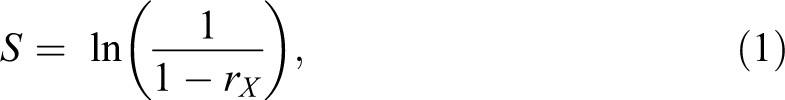
where S denotes status, X as before denotes the valued good (attribute or possession), and r denotes the relative rank on the valued good. Although the valued good can be either cardinal or ordinal, the status function notices only its relative rank. Sørensen (1979) provides strong rationale for this particular function, noting its relation to the exponential distribution.

In the case of comparison processes, Jasso (1978, 1990) proposed the log-ratio function:

Z = θ ln (\frac{X}{X^{*}}),

2.1

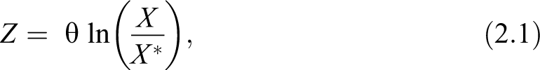
where Z denotes any of the comparison outcomes, such as self-esteem or the justice evaluation, X is as above the valued attribute or possession (called in this literature the actual reward), X* denotes the comparison referent (called the just reward in the special case of justice), and θ is the signature constant whose sign indicates whether the reward is viewed as a good or as a bad and whose absolute value denotes expressiveness. When the actual reward equals the comparison referent, the outcome is zero (a neutral point which in the case of justice is called the point of perfect justice); when the actual reward exceeds the comparison referent, the outcome is positive (representing overreward), and when the actual reward is less than the comparison referent, the outcome is negative (representing underreward). The log-ratio function has several useful properties, including scale-invariance and the property that deficiency is felt more keenly than comparable excess (now more commonly known as loss aversion), long considered central to matters of justice (Adams 1963:426, 1965:282; Brown 1986:78; Homans 1961:75-76; Wagner and Berger 1985:719). A summary of the nine properties identified to date appears in Jasso (2015:442-43).¹²

The actual reward in the comparison function is often denoted A instead of X, and the comparison referent C instead of X*. In the special case of justice, the comparison function is called the justice evaluation function, as originally proposed (Jasso 1978), and written:

J = θ ln (\frac{A}{C}),

2.2

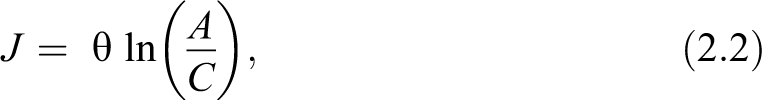
where J denotes the justice evaluation.

Finally, the power PSO is represented by a linear function:

P = a + b X,

where P denotes power and a and b are the intercept and slope, respectively. In the special case in which the intercept is 0 and the slope is 1, the function reduces to an identity function.

When the PSO is status or when the valued goods are ordinal (or the ordinal aspect of cardinal goods), qualitative characteristics provide the group or population within which the relative ranks are measured. As well, in the justice case, when the comparison referent is a summary characteristic of a distribution (such as the average or the median), qualitative characteristics provide the group or population within which the referent is measured. For example, those groups may be specified as a category of gender, nativity, religion, and so on.¹³

The Multiple-Input Primordial Sociobehavioral Outcome

Suppose that several goods are simultaneously valued. This can be any combination, such as several ordinal goods or several cardinal goods or a mix of both. Or suppose that two or three PSOs are activated, whether about the same good or about different goods. In these cases, the multiple-input PSO, denoted T, is written as the weighted sum of the component PSOs, with each component PSO denoted by the generic Y (which can represent the comparison outcome Z, status S, and power P), where w denotes the weight of each component PSO. In this case, the distributional form of T,

T = \sum_{i = 1}^{k} w_{i} Y_{i},

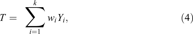
depends not only on the distributional forms of the Ys but also on their associations.¹⁴

Selecting the Modeling Distributions for the Personal Quantitative Characteristics

Consistent with the general framework (subsection on Selecting the Modeling Distributions for the Inputs), the personal quantitative characteristics are modeled by the unit rectangular if they are ordinal and by the lognormal, Pareto, and power-function if they are cardinal. Equally distributed quantitative characteristics are modeled by the equal distribution.¹⁵ Together, this set is useful for modeling a wide range of societies across time and space.

The QF, one of the associated functions of probability distributions introduced above, is especially useful in this application, for it expresses a value x as a function of the relative rank—for example, income amount as a function of relative rank in the income distribution, as in Pen’s (1971) Parade.

This set of modeling distributions has two further useful features. First, the power-function includes as a special case the rectangular distribution which represents a distribution of relative ranks, so that the three distributions provide models for both ordinal and cardinal goods. Second, given that all three distributions are continuous univariate two-parameter distributions, one of their two parameters is the general inequality parameter which governs all measures of inequality, so that in many of the analyses below, it will not be necessary to examine several measures of inequality, as all are monotonic functions of this one parameter.

In the spirit of van der Vaart (1968:294) and Gastwirth (1972:307), all quantities and formulas obtained below are reported by distributional form.

Deriving the Distributions of Sociobehavioral Outcomes Generated by Personal Attributes and Possessions

The PSOs can be generated by a single valued good or by multiple valued goods. In both cases, the distribution(s) of the valued good(s) determine(s), together with the PSO function, the distribution of the PSO. We consider the two cases separately, because they require different methods for deriving the PSO distributions.¹⁶

Deriving the PSO distribution in the single-good case

In the single-good case, obtaining the distribution of the sociobehavioral outcome can be immediate—as when the PSO is status—or somewhat elaborate—as when the PSO is justice and X and X* both vary—or intermediate—as when the PSO is justice and the comparison referent is the same for everyone.

X equal

If X is equally distributed and the PSO is status or power or justice (the latter with X* constant—namely, everyone has the same comparison referent), then the PSO is also equal.

Status PSO

As Sørensen (1979) noted, the status distribution is a standard negative exponential. To see this, look at the formula for the status function given in (1). As shown, status is an increasing function of relative rank. It is thus a QF, and it is instantly recognized as the QF of the standard negative exponential (see, e.g., Forbes et al. 2011:88).

Justice PSO with X* constant and power PSO

In these two cases, given the PDF of the good X and given the PSO function, the change-of-variable technique introduced in the subsection on Distribution of a Function of One Variable yields the PSO distribution.

Because the power PSO is a linear function of X, as shown in equation (3), its distribution is often immediate. For example, if X is rectangular, so is the power PSO distribution; and if the intercept in the power PSO function is 0, the PSO distribution is a scale transformation of the X distribution.

In the comparison distribution, if the referent amount X* is a fixed constant, then a simple change-of-variable procedure yields the outcome distribution, exactly as in the case of the power PSO. The comparison referent is a fixed constant in at least two substantively important cases: (1) the justice-is-equality case (words spoken by Socrates in Plato’s ([c.428-348/7 BC] 1952) Gorgias), where equality is represented by the arithmetic mean; and (2) the case in which each person compares to everyone else (Diekmann 2004:492), a case for which it can be shown that as the population size increases, the average of these referent amounts approaches the geometric mean.¹⁷

Justice PSO with X equal and X* varying

If X is equal and X* varies, a change-of-variable on X* yields the justice PSO distribution. Substantively, this is a rich case, arising, for example, if income is equally distributed but the principles of justice are meritocratic. As will be further discussed below, people will find it unjust that everyone is paid the same even though some may be more productive (or have greater need or longer tenure, etc.) than others.¹⁸

Justice PSO with X and X* both varying

To find the distribution of the justice PSO in this case, we use the method described in the general framework (subsection on Distribution of a Function of Several Variables). Note that when the X and X* distributions are identical, “identical” pertains to the distribution and not to the allocation to particular individuals.

Behaviorally, the case of X and X* varying, identical, and perfectly positively associated—that is, where, for each person X equals X*—is unusually rich. It is consistent with several scenarios in philosophy and social science, such as: First, the individual sets the comparison standard X* equal to the actual amount X, following the Stoic prescription to “want what you have.” Second, the individual follows the hedonic prescription to “get what you want,” manipulating X so that it exactly matches X*. Third, following Homans (1976:244), “what is, is always becoming what ought to be,” so that society anoints as just the prevailing allocation. Fourth, following Lerner (1980), the individual may have a need to believe that the world is just. Fifth, the view may arise that whatever people get on the market is fair. As can immediately be seen, this case of identical and perfectly positive association leads to an equal PSO distribution. For each individual, X equals X*, and thus for all individuals, Z equals 0. Together, the justice PSO cases examined here highlight the wide variety of sources of comparison referents (Evans, Kelley, and Peoples 2010; Jasso 2008b:270-73; Jasso 2016:191-92; Jasso 2021; Liebig and Sauer 2016), exemplifying the Hatfield–Friedman Principle that justice is in the eye of the beholder (Friedman 1977; Walster, Berscheid, and Walster 1973).¹⁹

Results—The PSO distributions

The variate families of the PSO distributions for the major one-good cases with ordinal or cardinal inputs and, if cardinal, with three alternative modeling distributions are widely available. For the reader’s convenience, these are collected in Tables A.1.a and A.1.b in the Online Appendix. Online Appendix Table A.1.b also reports distribution-independent results for the case in which justice is the PSO and both X and X* vary.

Figure 1A provides graphs of the QF associated with each of the distributions in Online Appendix Table A.1.a. Figure 1A is arranged exactly like Online Appendix Table A.1.a. The leftmost column depicts the input distribution, and the three columns to the right depict the three PSO distributions. In the case of ordinal goods, there is only one possible distribution, the unit rectangular, and only one PSO distribution. In the case of cardinal goods, however, the input distributions may have different parameters, and so, too, the PSO distributions. For simplicity, graphs depict one member from each variate family. All the graphs include a horizontal line at the arithmetic mean.

Figure 1A.

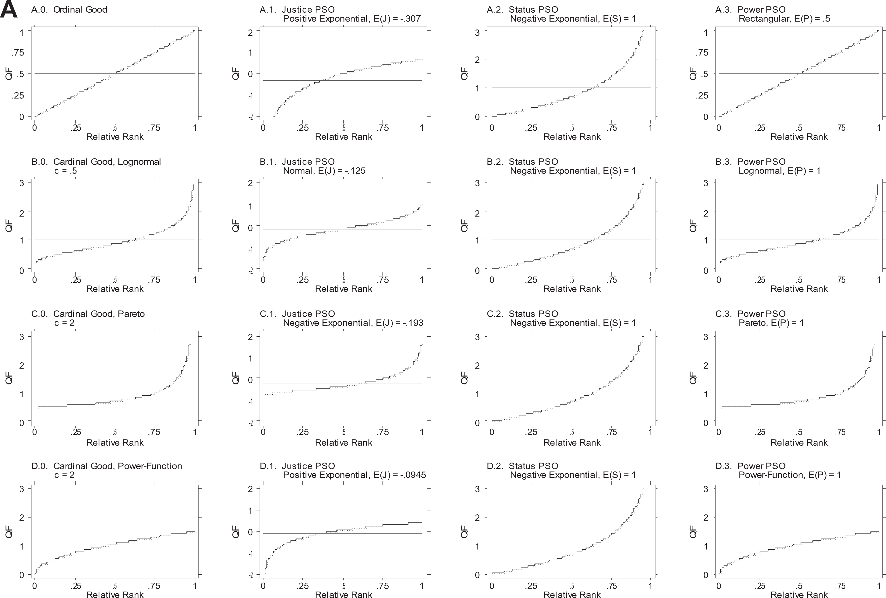
Quantile function of primordial sociobehavioral outcome (PSO) distributions arising from valued goods, with cardinal goods modeled by three variates: single-good case. The distributions of the valued goods are in the .0 column and the PSO distributions in the .1, .2, and .3 columns. The justice PSO distribution is in the .1 column, the status PSO distribution in the .2 column, and the power PSO distribution in the .3 column. The justice PSO distributions pertain to the case where the comparison referent X* is constant. All the graphs include a horizontal line at the arithmetic mean.

Each distribution provides a picture of society. The distributions in the leftmost column provide pictures of the first world, and the distributions in the second through fourth columns provide pictures of the second world. Given representation by the QF, the graphs have the appealing property that at a glance they reveal three important features: (1) each person’s position in the hierarchy, (2) who gains and who loses across different variates, and (3) the degree of inequality. In the equal distribution the QF is a horizontal line; in the other distributions, the flatter the curve, the lower the inequality. In Figure 1A, the horizontal line at the arithmetic mean can be interpreted as the QF of an equal distribution.

Online Appendix Table A.1.b provides the justice PSO distributions for the six cases where both X and X* vary. Figure 1B provides graphs of the QF associated with each of the distributions in Online Appendix Table A.1.b that arise when X and X* are identical. Following the pattern in Online Appendix Table A.1.a and Figure 1A, Figure 1B is arranged like panel C of Online Appendix Table A.1.b.

Figure 1B.

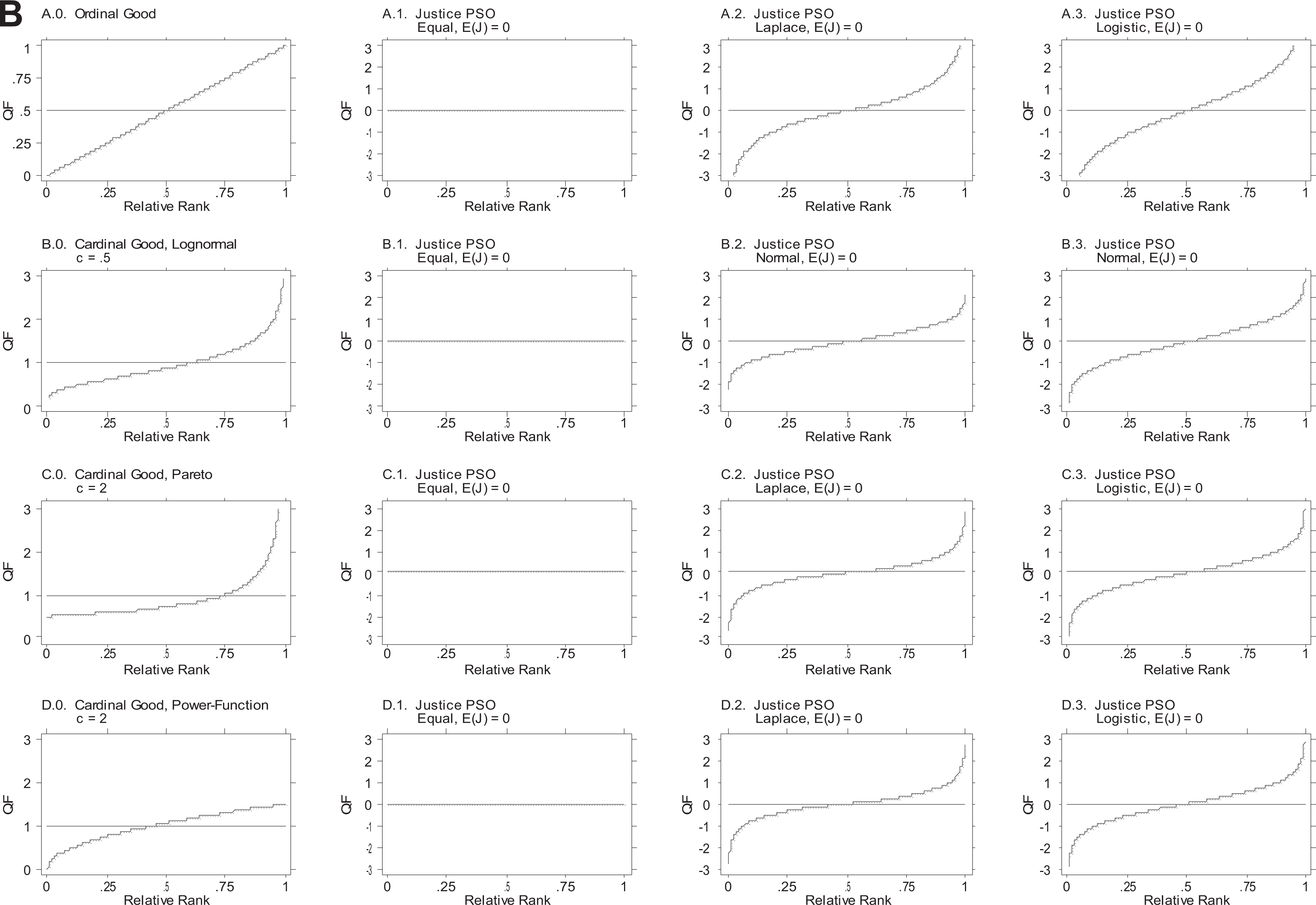
Quantile function of justice PSO distributions arising from valued goods, with cardinal goods modeled by three variates: single-good case, where X and X* are identical and both vary. The distributions of the valued goods are in the .0 column and the justice PSO distributions in the .1, .2, and .3 columns. X and X* are perfectly positively associated in the .1 column, independent in the .2 column, and perfectly negatively associated in the .3 column. All the graphs include a horizontal line at the arithmetic mean.

As shown in Online Appendix Tables A.1.a and A.1.b and in Figures 1A and 1B, the outcome PSO distributions include the normal, both negative and positive exponentials, the Laplace in both symmetric and asymmetric versions, the logistic and quasi-logistic, and the equal distribution. Thus, we started with three simple and plausible distributions to model the inputs of the first world—with and without a safety net and with and without a maximum—and they generated a large variety of other distributional forms for the sociobehavioral outcomes of the second world, many of which would not ordinarily be considered as models for the sociobehavioral world.

The distribution-independent results for the case in which justice is the PSO and both X and X* vary (panel A of Online Appendix Table A.1.b) are particularly illuminating. When X and X* are identical, the outcome distribution is centered on zero—the point of perfect justice, or, alternatively, the neutral point separating overreward and underreward—and the distribution is either symmetric or equal. However, when X and X* differ, the justice distribution may be symmetric or asymmetric about any number.

Deriving the PSO distribution in the multiple-good case

Procedures

As shown in equation (4) in the subsection on The Multiple-Input Primordial Sociobehavioral Outcome, the multiple-input PSO, denoted T, is the weighted sum of the component PSOs. Accordingly, to derive the multiple-good PSO distribution, the procedure is to take the weighted sum of the single-good PSO distributions. For example, if status arises from two goods—say, beauty and wealth, or athletic skill and musical skill—then the final PSO distribution is the weighted sum of the two single-good PSO distributions. For simplicity, we focus on the equally weighted case.

We again follow the strategy for combining distributions introduced in the subsection on Distribution of a Function of Several Variables, deriving the PSO distribution for six ideal-type multiple-good cases. For example, suppose that a population values both beauty and intelligence; because both are ordinal, the single-good PSO distributions are identical, but the two-good PSO distribution (and its inequality) will differ depending on whether beauty and intelligence are perfectly positively associated or independent or perfectly negatively associated.

Distribution-independent results

Results obtained to date include three distribution-independent results. The first two pertain to the case where the single-good distributions are identical. First, in the identical and perfectly positively associated case, the final multiple-good PSO distribution remains the same as the component single-good PSO distributions. Second, in the identical and perfectly negatively associated case, if the single-good distributions are symmetric, the final multiple-good PSO distribution collapses to the equal. Examples include cases where the single-good PSO distributions are identical normal, Laplace, or logistic (such as the justice PSO distributions arising from lognormal, Pareto, and power-function goods, shown in Online Appendix Tables A.1.a and A.1.b. The third result pertains to symmetric, perfectly negatively associated PSO distributions that differ but are related to each other by the addition or subtraction of a constant; in this case, their average collapses to the equal, exactly as if they were identical.

Distribution-specific results—Normal single-good PSO distributions

The single-good PSO distributions in Online Appendix Tables A.1.a and A.1.b include several normals, not necessarily identical. A well-known theorem on linear combinations of independent normal variables immediately yields this result: If the single-good PSO distributions are independent normals, then the final multiple-good PSO distribution is also normal.

Distribution-specific results—Negative exponential single-good PSO distributions

In this case, the multiple-good PSO distribution remains negative exponential if the goods are perfectly positively associated, becomes Erlang if the goods are independent, and becomes the mirror-exponential if multiple goods are negatively associated (Jasso and Kotz 2007).

This approach can be extended to the positive exponentials in Online Appendix Tables A.1.a and A.1.b.

Other multiple-good PSO distributions may prove more difficult to derive or may yield new distributional forms. However, even if the distributional form is difficult to derive, it will still be possible to work with its variance—given the arsenal of useful theorems on variances—and thus analyze the inequality connection across the two worlds.

How Do the Mechanisms for Generating and Altering Inequality Differ Across the Two Worlds?

Inequality in the First World

Measures of inequality in the first world

As discussed above, the input variables in this application are positive, and they are modeled by the unit rectangular, lognormal, Pareto, and power-function variates. Formulas for measures of inequality among the latter three are widely available (e.g., Jasso 2018:201). In the rectangular, inequality is fixed and unchanging. For example, the Gini coefficient is one third; the Atkinson inequality is 1 − (2/e), or approximately .264; the Theil MLD is 1 − ln(2), or approximately .309; and the coefficient of variation is always $1 / \sqrt{3}$ .²⁰

In the three modeling distributions for cardinal goods, as noted above, inequality is governed by the general inequality parameter c, with all inequality measures being monotonic functions of c. Inequality is a decreasing function of c for the Pareto and the power-function variates and an increasing function of c for the lognormal. In the Pareto, the variance, and hence the CV, is defined only for c > 2.

How to change inequality in the first world

The question arises: How does inequality work? What operations can make inequality increase or decrease? The literature discusses two sets of operations, the first based on properties of inequality measures, the second on behavioral models (Jasso 2018:187-92). Examples of the first include transfers to/from richer and poorer persons—inequality decreasing with transfers from relatively richer persons to relatively poorer persons—and addition/subtraction of a fixed constant—inequality decreasing with addition of a fixed constant to all incomes (Dagum 1983). These operations apply only to material possessions, not to attributes like beauty or skill. Examples of the second include assortative mating—inequality decreasing when rich marry poor (Jencks et al. 1972:74, 211, 233-34, 271-73; Plato ([c.428-348/7 BC] 1952), Laws VI, 773). However, the negative assortative mating solution to inequality has the disadvantage that it increases inequality between spouses.

Inequality in the Second World

Measures of inequality in the second world

The attributes and possessions of the first world are represented by positive numbers and thus their inequality can be measured by the full set of inequality measures. In the second world, however, only two of the three sociobehavioral outcomes—status and power—can be represented by positive numbers alone. Moreover, depending on the sign of the intercept and the exact configuration of the elements of the power PSO function shown in equation (3), the power PSO can also assume negative values. Accordingly, while status and sometimes power are amenable to inequality measurement using the usual measures, for measuring inequality in the comparison PSOs, as well as in some power PSOs, we rely on the variance and the GMD, measures which are applicable to variables that span both negative and positive numbers. Contrasts based on the variance and the GMD are straightforward when the distributions have the same arithmetic mean.

Table 2 reports the formulas for the variance and the GMD in the distributions of the justice, status, and power sociobehavioral outcomes, for the case of ordinal goods and cardinal goods, the latter modeled by the three variates explored in this article (the lognormal, Pareto, and power-function). For ease in using Table 2, the PSO functions are shown underneath the PSO name. For simplicity, the formulas for the justice PSO pertain to the case in which the comparison standard X* is a constant (such as the arithmetic mean or geometric mean). The variate families of the PSO distributions for the cases in Table 2 are shown in Online Appendix Table A.1.a. For example, the status PSO is a standard negative exponential, and when the cardinal good is lognormal, the justice PSO is normal.²¹

Table 2.

Inequality in the Second World: Formulas for Two Measures of Inequality in the PSO Distributions That Arise From the Modeling Distributions for Attributes and Possessions.

X Variate	Primordial Sociobehavioral Outcome
	Justice		Status		Power
	$Z = ln (\frac{X}{X^{*}})$		$S = ln (\frac{1}{1 - r_{X}})$		$P = a + b X$
	Var(Z)	GMD(Z)	Var(S)	GMD(S)	Var(P)	GMD(P)
A. Ordinal good
Rectangular	1	1	1	1	$\frac{b^{2}}{12}$	$\frac{b}{3}$
B. Cardinal good
Lognormal	c ²	$\frac{2 c}{\sqrt{π}}$	1	1	$b^{2} μ^{2} [exp (c^{2}) - 1]$	$2 b μ [2 F_{N} (\frac{c}{\sqrt{2}}) - 1]$
Pareto	$\frac{1}{c^{2}}$	$\frac{1}{c}$	1	1	$\frac{b^{2} μ^{2}}{c (c - 2)}$	$\frac{2 b μ}{2 c - 1}$
Power-Function	$\frac{1}{c^{2}}$	$\frac{1}{c}$	1	1	$\frac{b^{2} μ^{2}}{c (c + 2)}$	$\frac{2 b μ}{2 c + 1}$

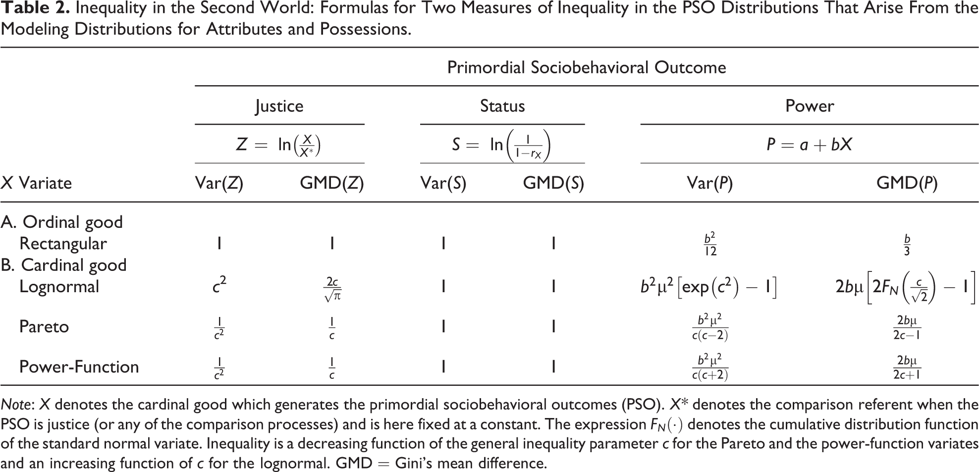
Note: X denotes the cardinal good which generates the primordial sociobehavioral outcomes (PSO). X* denotes the comparison referent when the PSO is justice (or any of the comparison processes) and is here fixed at a constant. The expression $F_{N} (\cdot)$ denotes the cumulative distribution function of the standard normal variate. Inequality is a decreasing function of the general inequality parameter c for the Pareto and the power-function variates and an increasing function of c for the lognormal. GMD = Gini’s mean difference.

For visual illustration, Figures 2A and 2B provide graphs of the variance and GMD, respectively, in the PSO distributions for the three variates arising from the cardinal goods, expressed as functions of the general inequality parameter c of the good’s distributions.

Figure 2A.

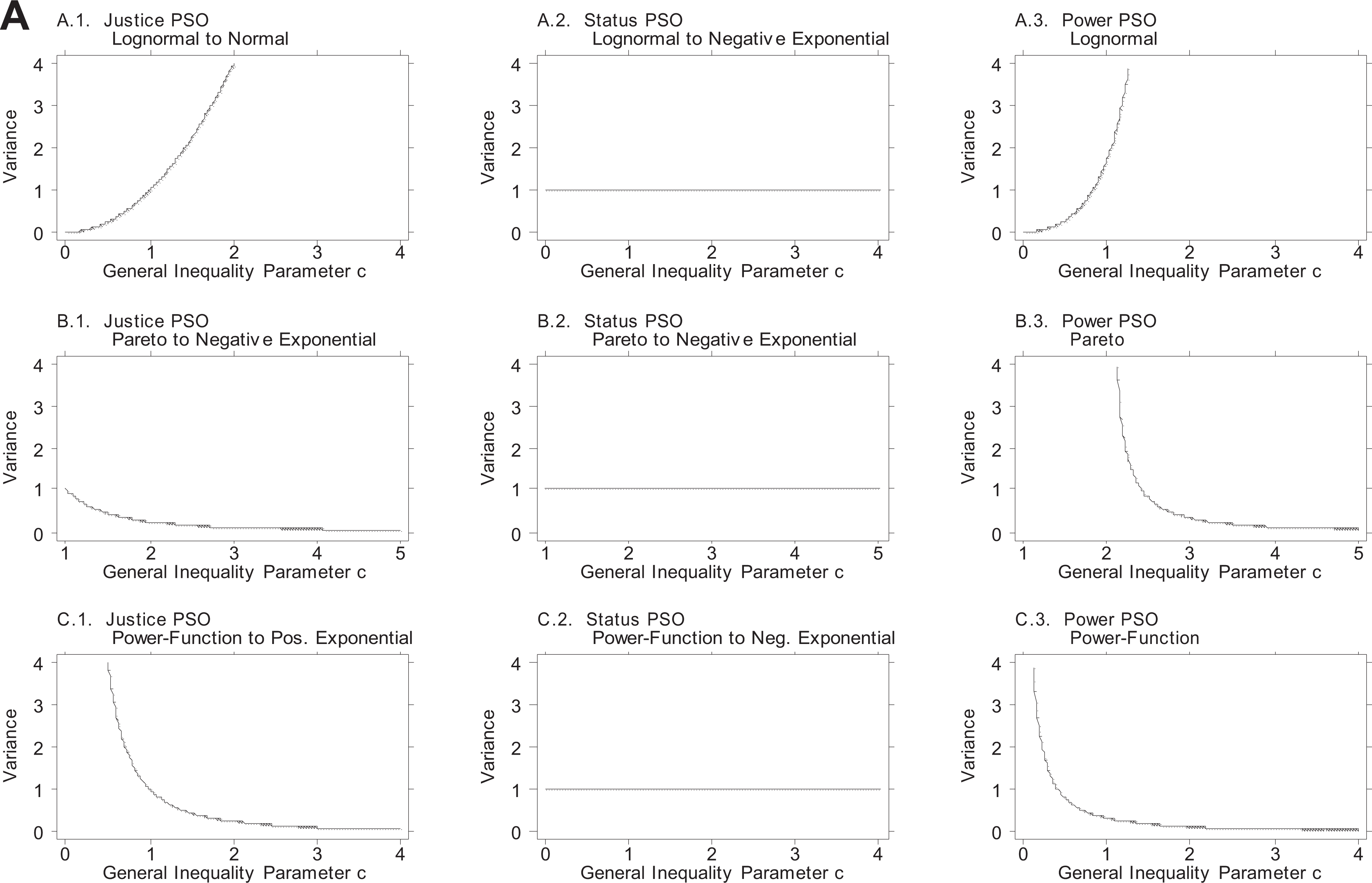
Variance in the primordial sociobehavioral outcome (PSO) distributions arising from valued cardinal goods, with the goods modeled by three variates: single-good case. As in Figure 1A, the justice PSO distribution is in the .1 column, the status PSO distribution in the .2 column, and the power PSO distribution in the .3 column.

Figure 2B.

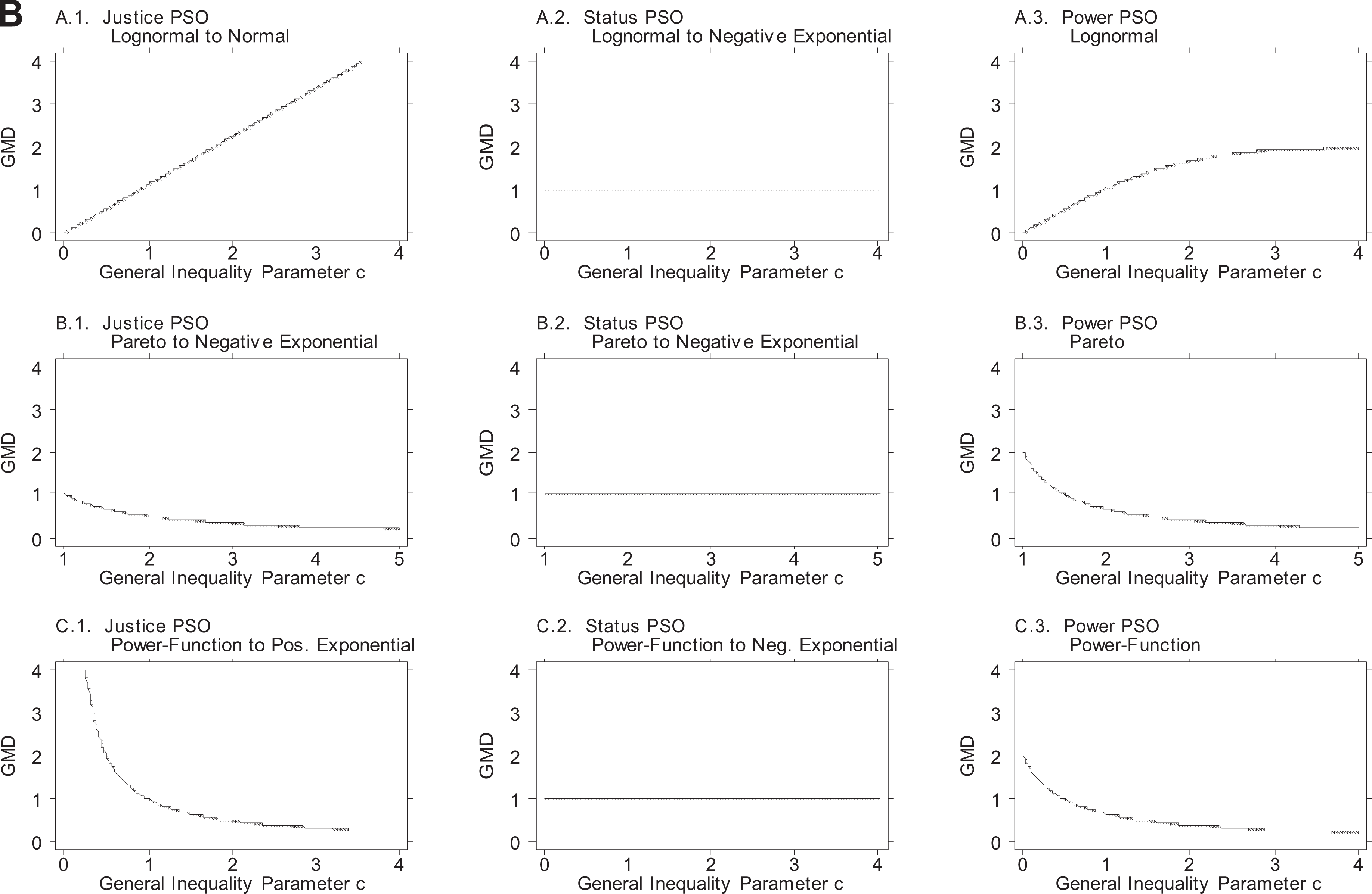
Gini’s mean difference (GMD) in the PSO distributions arising from valued cardinal goods, with the goods modeled by three variates: single-good case. As in Figures 1A and 2A, the justice PSO distribution is in the .1 column, the status PSO distribution in the .2 column, and the power PSO distribution in the .3 column.

There are several important results in Table 2 and Figures 2A and 2B. First (and this immediately hits the eye), when status is the active force, the variance and GMD are fixed (as shown in the middle columns of Table 2 and Figures 2A and 2B. Second (and this, too, hits the eye in Table 2), when the valued goods are ordinal (or cardinal goods treated ordinally), the variance and GMD are again fixed, except for the operation of the slope b in the power PSO function. Third, when the valued goods are cardinal and the active PSO is justice or power, the PSO variance and GMD are monotonic functions of the cardinal good’s general inequality parameter c, and thus, previewing the sixth section, inequality in the second world is a monotonic function of inequality in the first world. Fourth, when the active PSO is power, the slope b of the power PSO function operates as a multiplier, intensifying or attenuating inequality in the second world.

Thus, Table 2 and Figures 2A and 2B show that for given inequality in an attribute or possession, the experience of inequality in the second world differs substantially by PSO, by type of valued good (cardinal or ordinal), by the form and inequality of valued cardinal goods, and by combinations thereof. The sixth section uses the information in Table 2 and Figures 2A and 2B to assess the link between income inequality and PSO inequality.

Observe that the first two results highlighted above are visible as a T formation in Table 2, and the first result as the stem of a T in Figures 2A and 2B.²²

Justice PSO when both X and X* vary

The foregoing justice PSO results pertain to the class of justice PSO distributions that arise when the comparison standard (or just reward) X* is constant. When both X and X* vary, inequality in the justice PSO is a function of inequality in both the X and X* distributions. Moreover, as seen in Online Appendix Table A.1.b, the justice PSO distribution depends on whether X and X* are identical or different and on whether they are positively or negatively associated or independent. Here, we report a distribution-independent result and several distribution-specific results.

Table 3, panel A, reports the formulas for the variance of the justice PSO distribution for the six ideal-typical cases combining X and X*. As shown, when X and X* are identically distributed, the variance is zero in the perfectly positively associated case, increases to double the variance of ln(X) in the independent case, and increases still more in the perfectly negatively associated case.

Table 3.

Inequality in the Second World: Variance in the Justice PSO Distribution, Single-Good Case, where X and X* Both Vary.

X, X* Variates	Association Between X and X*
X, X* Variates	Perfect Positive	Independent	Perfect Negative
A. Distribution-independent results
Identical	0	$2 Var [ln (X)]$	$2 Var [ln (X)] \times (1 - ρ)$
Different	$Var [ln (X)] + Var [ln (X^{})]$ $- 2 Cov [ln (X)], ln (X^{})$	$Var [ln (X)] + Var [ln (X^{*})]$	$Var [ln (X)] + Var [ln (X^{})]$ $- 2 Cov [ln (X)], ln (X^{})$
B. Ordinal good
Identical	0	2	$\frac{π^{2}}{3} \approx 3.29$
C. Cardinal good
Lognormal
Identical	0	$2 c^{2}$	$4 c^{2}$
Different	${(c_{X} - c_{X^{*}})}^{2}$	$c_{X}^{2} + c_{X^{*}}^{2}$	${(c_{X} + c_{X^{*}})}^{2}$
Pareto or power-function
Identical	0	$\frac{2}{c^{2}}$	$\frac{π^{2}}{3 c^{2}} \approx \frac{3.29}{c^{2}}$
Different	$\frac{{(c_{X} - c_{X^{}})}^{2}}{c_{X}^{2} c_{X^{}}^{2}}$	$\frac{{(c_{X} - c_{X^{}})}^{2}}{c_{X}^{2} c_{X^{}}^{2}} + \frac{2}{c_{X} c_{X^{*}}}$	$\frac{{(c_{X} - c_{X^{}})}^{2}}{c_{X}^{2} c_{X^{}}^{2}} + \frac{π^{2}}{3 c_{X} c_{X^{*}}}$

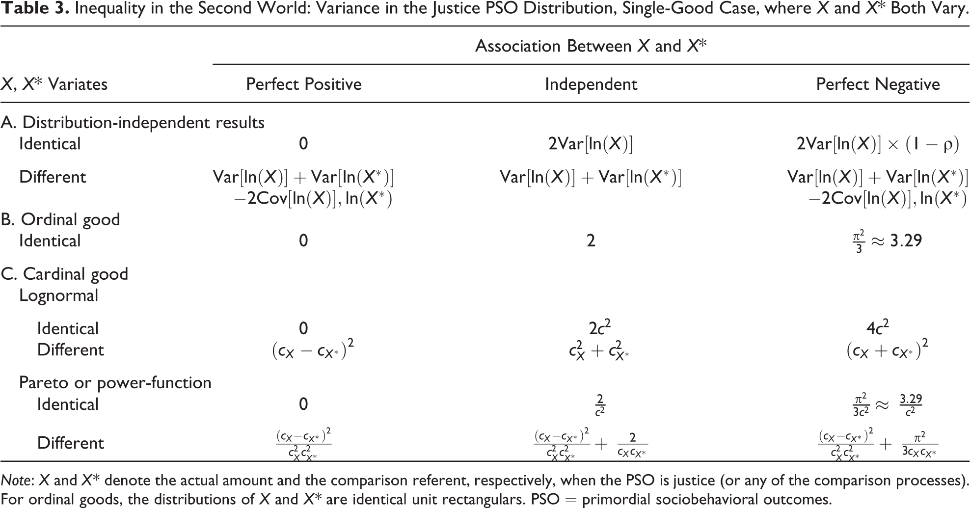
Note: X and X* denote the actual amount and the comparison referent, respectively, when the PSO is justice (or any of the comparison processes). For ordinal goods, the distributions of X and X* are identical unit rectangulars. PSO = primordial sociobehavioral outcomes.

Table 3 also reports results for the cases where X and X* are rectangulars, lognormals, Paretos, and power-functions. As shown, when X and X* are identical lognormals, the variances of the justice PSO distribution are zero, 2c², and 4c² in the perfectly positively associated, independent, and perfectly negatively associated cases, respectively. Because the ln(X) and ln(X*) distributions are symmetric, their correlation in the perfectly negatively associated case is −1, yielding a variance that is four times the variance of ln(X)—shown in Table 2, panel B, and Table 3, panels A and C. The situation differs in two ways when X and X* are identical Paretos or power-functions. First, as shown in Online Appendix Table A.1.b, the justice PSO distributions differ in the independent and perfectly negatively associated cases, becoming Laplace in the former and logistic in the latter. Second, the variances increase to 2/c² in the Laplace and π²/3c² (approximately 3.29/c²) in the logistic but do not reach four times the variance of ln(X)—because the ln(X) and ln(X*) distributions are not symmetric and thus their correlation does not reach −1. In all cases, however, the increase in the variance, as X and X* move from perfect positive association to independence to perfect negative association, is illuminating.

How to change inequality in the second world

The preceding section identified two situations in which second-world inequality is zero—namely, (1) when X is equal, and if justice is the PSO, X* is not fixed (subsection on Deriving the PSO Distribution in the Single-Good Case); and (2) when justice is the active force, the comparison reward X* is fixed, and X and X* are identical and perfectly positively associated (as, e.g., in the Stoic and hedonic scenarios for selecting a comparison referent discussed in the subsection on Deriving the PSO Distribution in the Single-Good Case)—and two situations in which second-world inequality is nonzero but constant—namely, (1) when an ordinal good is valued, and (2) when status is the active force. In other situations—such as when (1) a cardinal good is valued, and either (2.a) justice is the active force and the comparison referent is fixed or (2.b) justice is the active force and X and X* are identical and independent or perfectly negatively associated or (2.c) power is the active force—second-world inequality depends on first-world inequality, and whatever affects first-world inequality also affects second-world inequality.²³

Are there other mechanisms for altering inequality in the second world? Yes. As Berger, Cohen, and Zelditch (1966) showed over 50 years ago, an important key to reducing inequality in outcomes of the second world is for people to value multiple goods that are not perfectly positively associated.

Multiple-good effects on inequality in the second world

Suppose that multiple goods are simultaneously valued. The multiple goods may be different attributes or possessions or different dimensions of attributes or possessions—for example, two types of knowledge, or the not uncommon income and athletic skill or historical pairs like military skill and horsemanship or the staple of baseball reporting, batting and fielding. Valuing multiple goods whose distributions are all perfectly positively associated has no impact on the PSO distributions of the second world. But valuing multiple goods whose distributions are independent or negatively associated substantially reduces inequality. In fact, even valuing multiple goods which are positively associated—but not perfectly positively associated—reduces inequality, though not as much as when they are independent or negatively associated. At one extreme, valuing two goods which are perfectly negatively associated and whose single-good PSO distributions are either symmetric or related by addition/subtraction of a constant completely destroys inequality (subsection on Deriving the PSO Distribution in the Multiple-Good Case).

To see this multiple-good effect on PSO inequality, we examine the variance in the multiple-good PSO distribution T introduced in the subsection on The Multiple-Input Primordial Sociobehavioral Outcome, expressed in equation (4), and developed in the subsection on Deriving the PSO Distribution in the Multiple-Good Case. The arithmetic mean of the multiple-good PSO remains the same regardless of the associations among the component single-good PSOs. Accordingly, examination of the variances will shed light on multiple-good effects. We again make use of the six ideal types introduced in the subsection on Distribution of a Function of Several Variables, working with the associated variances.

The case of multiple goods with identical distributions

In the simplest case, the multiple goods have identical distributions and the active PSO, denoted Y as before—to cover all three PSOs—is the same for all the goods. In this case, the single-good PSO distributions are identical, with variance Var(Y). If the multiple goods are perfectly positively associated, the final PSO distribution will have the same variance as each of the input PSO distributions, namely, Var(T) equals Var(Y). If the multiple goods are statistically independent, however, the variance of the final PSO distribution drops to [Var(Y)]/N. And if the goods are negatively associated, the variance in the final PSO distribution drops still more.

The case of two goods with identical distributions

To show more vividly the reduction in inequality that comes with valuing negatively associated goods, consider the special case of two identical goods and, as immediately above, the same PSO. In this case, the formula for the variance reduces to [Var(Y)][1 + ρ]/2. If the correlation ρ between the two single-good PSO distributions equals −1 (e.g., when they are symmetric), the variance of the final multiple-good PSO distribution equals zero.

What would such a situation look like? Suppose that all the members of a group or population (children, at home or at summer camp; graduate students; and military recruits) each receive an allowance or stipend from each of two payers (two parents, say, or two professors or two commanders), and they value the two stipends equally. Suppose further that each of the two payers is restricted to the same fixed schedule of payments. All results are as above. The variance of the final PSO distribution depends on the associations between the two single-good PSO distributions. For example, if the payment schedule is lognormal and the PSO is justice (with the comparison referent X* constant), the single-good PSO distributions are normal (Online Appendix Table A.1.a), and thus symmetric, so that if the two payment distributions are perfectly negatively associated, the two single-good PSO distributions have a correlation of −1 and the final PSO distribution has a variance of zero.

The case of two goods with different but equal-variance PSO distributions

It is straightforward to show that even if the two goods differ, if the PSO distributions have the same variance, the two-good PSO declines in the same way as when the two single-good PSOs have identical distributions.

As a simple example, consider the same scenario as above, with two payers, the justice PSO, and lognormal fixed payment schedules. Suppose that the comparison referent differs across the two payers, remaining fixed within each payer distribution. In this case, the two single-good PSO distributions will be different normals with the same variance. Results are the same as if the two single-good PSO distributions were identical normals.

The case of greater inequality reduction from independent goods than from negatively associated goods

Consider the case of multiple valued goods. If the goods are independent, the variance reflects the number of goods N and is equal to [Var(Y)]/N. But suppose they are organized into two subsets, as in the Berger et al. (1977) approach, such that within each subset all the goods are perfectly positively associated and the two subsets are perfectly negatively associated. The variance now reflects the number of subsets 2 and is equal to [Var(Y)][1 + ρ]/2. By algebraic manipulation, it follows that the two variances are equal when ρ equals [(2/N) − 1] and, more to the point, the independent-case variance is smaller when ρ exceeds [(2/N) − 1]. For example, if N, the number of goods is, 8—and, following the Berger et al. (1977) procedure, the eight goods are arranged in two subsets of four each, with perfect positive association within subsets—then the independent-case variance [Var(Y)]/8 will be smaller than the negative-case variance [Var(Y)][1 + ρ]/2 when the correlation between the two subsets exceeds [(2/8) − 1], or −.75. This would happen if ρ is −.7, say, or −.6, as can be readily verified.

Which of the Two Worlds Has More Inequality?

The foregoing analysis of the rules that govern inequality in each of the two worlds suggests that whether the first world or the second world has more inequality depends on the active PSO, the type of valued good(s), and the distributional form and inequality in valued cardinal goods, as well as the number of and associations among the valued goods. This section systematically contrasts inequality across the two worlds.

Given that in the second world the usual measures of inequality apply only to status and sometimes the power PSO, our strategy has two elements. First, we obtain and collect distribution-independent results. Second, we analyze contrasts involving distributions of the second world whose support is the positive half line. In this way, we obtain a large number of results that exemplify the great heterogeneity of the inequality connection across the two worlds. Of course, future work can fruitfully provide detailed analysis of special cases not covered here. For clarity, and as before, we examine separately the single-good and multiple-good cases.

Single Valued Good

Single valued good: Distribution-independent results

The case where first-world inequality is zero

The first general distribution-independent result is that if first-world inequality is zero, second-world inequality is also zero (Online Appendix Table A.1.a)—and inequality is the same in both worlds—except in the case where justice is the active PSO and the comparison referent X* varies. The exception would arise if, for example, income is equally distributed but the principles of justice are meritocratic, as discussed in the subsection on Deriving the PSO Distribution in the Single-Good Case. People will find it unjust that everyone is paid the same even though some may be more productive (or have greater need or longer tenure, etc.) than others. In this case, economic equality is unstable, vulnerable to efforts to achieve justice by introducing inequality.²⁴

The case where first-world inequality is nonzero and power is the PSO

The task is to contrast inequality in X with inequality in P. As shown in formula (3), P is a linear function of X, with intercept a and slope b. Accordingly, all inequality measures which are scale-invariant will be impervious to the slope b, and all inequality measures which display the principle of addition/subtraction of a constant discussed above will respond to the intercept a. In general, then, the sign of a determines whether relative inequality in the two worlds is the same or different and, if different, which is larger. To wit, if a is negative, inequality is greater in the second world, and if a is positive, inequality is greater in the first world.

The case where first-world inequality is nonzero, justice is the PSO, both X and X* vary, and their distributions are identical and perfectly positively associated

Notwithstanding the negative values in the support of the justice PSO distribution, there is one situation which readily yields an answer to the question, Which world has more inequality? This is the situation in which the justice PSO has no inequality at all. As shown in Online Appendix Table A.1.b, panel A, and discussed in the subsection on Deriving the PSO Distribution in the Single-Good Case, this situation arises when both X and X* vary and their distributions are identical and perfectly positively associated. Hence, in this case, inequality is lower in the second world than in the first world.

As noted in the subsection on Deriving the PSO Distribution in the Single-Good Case, this case is behaviorally rich, consistent with both scenarios in which X affects X* and scenarios in which X* affects X. Note also that when the first world has economic inequality and the second world has zero inequality, the second world provides refuge from the first world, and with it a casual accommodation with economic inequality that can retard or inhibit efforts to reduce it.

Inequality contrasts involving the one-good status PSO world

We turn now to the contrast between inequality in the valued good X and inequality in status S. X can be either ordinal or cardinal, but the status function notices only the ordinal dimension. The measures of inequality for the second world are shown in Table 2 (for the first world, they are widely available, as in Jasso 2018:201, 204). The status PSO has the property that its arithmetic mean is 1, so that the coefficient of variation is the same as the variance, and the Gini coefficient equals .5. Accordingly, the question which world has the greater inequality reduces to contrasting measures across the two worlds.

Table 4 reports the coefficient of variation and the Gini coefficient for both X and the status PSO, together with their contrast. As shown, when the valued good is ordinal, status always has more inequality than the ordinal good. However, as is intuitive, when the valued good is cardinal, the question whether the good or status has more inequality depends on the magnitude of inequality in the cardinal good’s distribution. Accordingly, for each variate and each inequality measure, we solve for the point at which the good and status have the same magnitude of inequality. For example, given that the Gini coefficient in the status distribution is constant at .5, any income distribution with a Gini greater than .5 will have more inequality than the status distribution, and, conversely, any income distribution with a Gini lower than .5 will have less inequality than the status distribution.

Table 4.

Which World Has More Inequality? Contrasting Inequality in X and Inequality in Status: Single-Good Case.

X Variate	Coefficient of Variation			Gini Coefficient
X Variate	X	Status	Which Is Greater?	X	Status	Which Is Greater?
A. Ordinal good
Rectangular	$\frac{1}{\sqrt{3}} \approx .577$	1	Status	$\frac{1}{3}$	.5	Status
B. Cardinal good
Lognormal	$\sqrt{[e x p (c^{2})] - 1}$	1	Statusif $c < \sqrt{ln (2)}$ ≈ .833	$2 F_{N} (\frac{c}{\sqrt{2}}) - 1$	.5	Statusif $c < \sqrt{2} Q_{N} (.75)$ ≈ .954
Pareto	$\frac{1}{\sqrt{c (c - 2)}}$	1	Statusif $c > 1 + \sqrt{2}$ ≈ 2.414	$\frac{1}{2 c - 1}$	.5	Statusif $c > 1.5$
Power-Function	$\frac{1}{\sqrt{c (c + 2)}}$	1	Statusif $c > - 1 + \sqrt{2}$ ≈ .414	$\frac{1}{2 c + 1}$	.5	Statusif $c > .5$

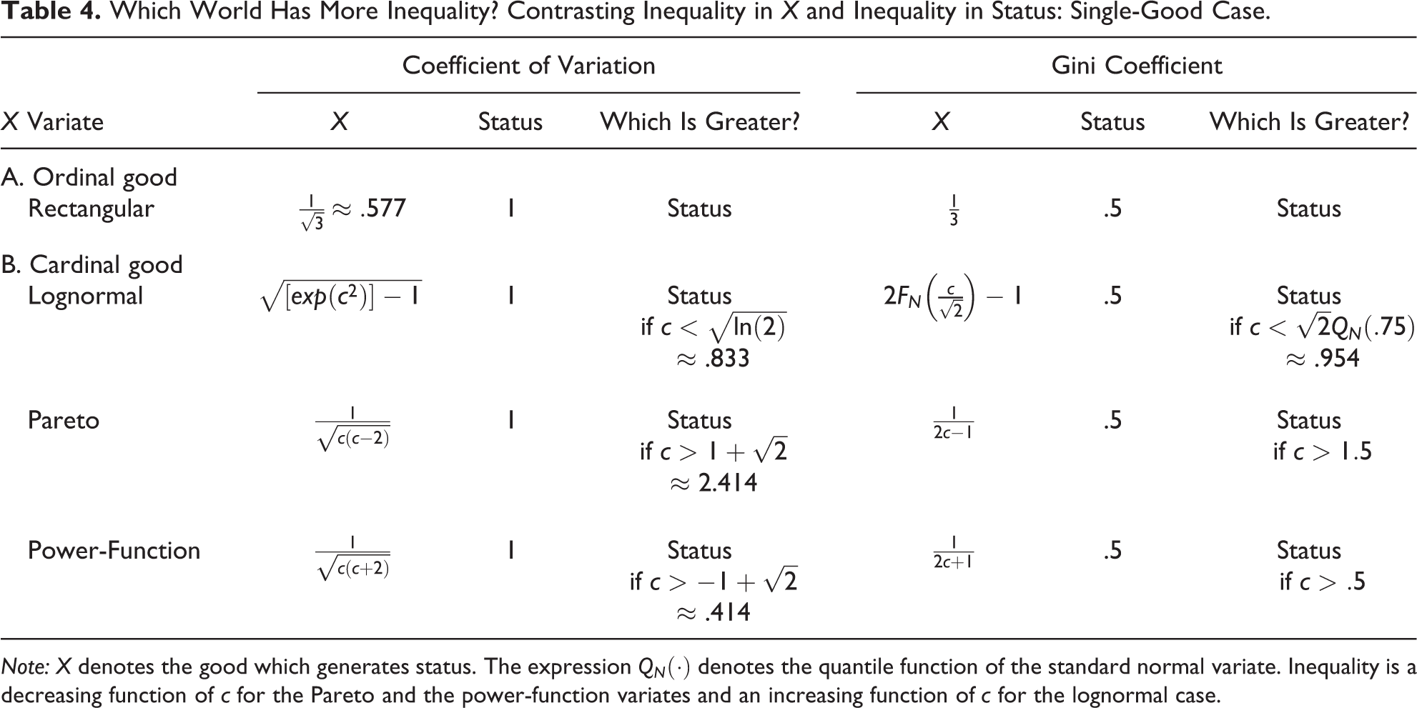
Note: X denotes the good which generates status. The expression $Q_{N} (\cdot)$ denotes the quantile function of the standard normal variate. Inequality is a decreasing function of c for the Pareto and the power-function variates and an increasing function of c for the lognormal case.

As shown in Table 4, the exact magnitude of inequality in the good’s distribution that renders it more or less unequal than status varies not only with the cardinal good’s distribution but also with the particular inequality measure. For example, when measured by the coefficient of variation, a Pareto distribution must have an inequality parameter greater than 2.414 in order for it to have less inequality than status, but when measured by the Gini coefficient, all that is required for the Pareto to have less inequality than status is for its inequality parameter to be greater than 1.5. What do such Pareto distributions look like? In the Pareto, the general inequality parameter c governs not only all measures of inequality but also other important features such as the lower extreme value (minimum income, say) and the proportion below the mean. As c increases, inequality declines, the lower extreme value increases, and the proportion below the mean increases. For example, at c = 1.5, the lower extreme value is one third of the mean, and the proportion below the mean is .808; at c = 2.414, the lower extreme value is .586 of the mean, and the proportion below the mean is .725.

Multiple Valued Goods

Multiple valued goods: Distribution-independent results

The case where one good’s inequality is zero

In this case, second-world inequality is nonzero—and the second world has more inequality than the one good whose inequality is zero—unless the configuration of the other goods yields a final PSO with zero inequality (discussed below). As a simple example, consider the case where two goods are valued, beauty and wealth; wealth is perfectly equally distributed but beauty is not. In this case, economic inequality in the first world is zero, but second-world inequality is nonzero.

The case where the valued goods are identically distributed and not perfectly positively associated

As seen in the subsection on How to Change Inequality in the Second World, when multiple goods are valued, if they are independent or negatively associated, PSO inequality declines. Indeed, inequality declines even if the multiple valued goods are positively correlated, provided the correlation is not perfect. To illustrate with the case of two identical goods, as the correlation of the two single-good PSO distributions moves from −1 to 0 to +1, the variance in the final PSO distribution, Var(T), moves from zero to [Var(Y)]/2 to Var(Y). The case of an imperfect positive correlation leads to a final PSO variance between [Var(Y)]/2 and Var(Y). The case of a perfect negative correlation leads to a final PSO variance of zero. Accordingly, there is less inequality in the second world than in the first world.

Inequality contrasts involving the two-identical-good status PSO world

If the two valued goods are identical and perfectly positively associated, the status distribution remains the same as in the one-good case—namely, the standard negative exponential which we already contrasted with the good’s inequality in Table 4 and in the subsection above on How to Change Inequality in the First World. When the two goods are independent, the status distribution becomes an Erlang (subsection on Deriving the PSO Distribution in the Multiple-Good Case), and the coefficient of variation declines to $1 / \sqrt{2}$ , or approximately .707, and the Gini coefficient to .375. When the two goods are perfectly negatively associated, the status distribution becomes a ring(2)-exponential (the two-good version of the mirror-exponential discussed in the subsection on Deriving the PSO Distribution in the Multiple-Good Case), and inequality declines further to approximately .422 in the CV and .193 in the Gini coefficient. Note that the negative exponential is not symmetric and thus the correlation between the two perfectly negatively associated exponentials does not reach −1; hence, inequality does not disappear from the final two-good status distribution.

To appreciate the decline in inequality as the two goods move from perfect positive association to independence to perfect negative association, note that the lower extreme value moves from zero in the standard exponential and the Erlang to ln(2), or approximately .693, in the ring(2)-exponential, and the mode moves from zero in the exponential to .5 in the Erlang to ln(2) in the ring(2)-exponential (Jasso and Kotz 2007:310). As to the curves’ shape, the graph of the PDF is downward-sloping in the exponential and the ring(2)-exponential, while in the Erlang it is an asymmetric mountain. Visualization of all three main associated functions is provided in Jasso and Kotz (2007:311-12). Substantively, these results provide a way to assess the impact of observed correlations on the status world and its inequality, from correlations of IQ and schooling, as in Jencks et al. (1972), to correlations between batting and fielding or between military skill and diplomatic skill or between athletic skill and musical skill. The little status worlds of everyday life have less inequality as the associations between the valued goods go from positive to negative.

To contrast inequality across the two worlds—and display the contrast—we construct two tables, one each for the coefficient of variation and the Gini coefficient. Each table collects the corresponding inequality formulas for the valued good X and for the status distribution in the two-goods/independent case and the two-goods/perfectly-negatively-associated case. To the right of each status inequality formula, there is, as in Table 4, a column for reporting the result of the contrast.

The case of two ordinal goods

We first contrast inequality in the status distribution with inequality in the ordinal-good distribution. As shown in Tables 5A and 5B, both the coefficient of variation and the Gini coefficient indicate that inequality is larger in the status distribution than in the ordinal-good distribution in the two-goods/independent case but larger in the good’s distribution in the two-goods/perfectly-negatively-associated case.

Table 5A.

Which World Has More Inequality? Contrasting Inequality in X and Inequality in Status: Two-Identical-Goods Case, With Inequality Measured by the Coefficient of Variation.

X Variate	Coefficient of Variation
		Two Goods Independent		Two Goods Perfectly Negatively Associated
	X	Status	Which Is Greater?	Status	Which Is Greater?
A. Ordinal good
Rectangular	$\frac{1}{\sqrt{3}} \approx 0.577$	$\frac{1}{\sqrt{2}} \approx 0.707$	Status	$\sqrt{0.178} \approx 0.422$	X
B. Cardinal good
Lognormal	$\sqrt{[exp (c^{2})] - 1}$	$\frac{1}{\sqrt{2}} \approx 0.707$	Statusif $c < \sqrt{ln (3 / 2)}$ ≈ 0.637	$\sqrt{0.178} \approx 0.422$	Statusif $c < \sqrt{ln (1.178)}$ ≈ 0.405
Pareto	$\frac{1}{\sqrt{c (c - 2)}}$	$\frac{1}{\sqrt{2}} \approx 0.707$	Statusif $c > 1 + \sqrt{3}$ ≈ 2.732	$\sqrt{0.178} \approx 0.422$	Statusif $c > 3.573$
Power-Function	$\frac{1}{\sqrt{c (c + 2)}}$	$\frac{1}{\sqrt{2}} \approx 0.707$	Statusif $c > - 1 + \sqrt{3}$ ≈ 0.732	$\sqrt{0.178} \approx 0.422$	Statusif $c > 1.573$

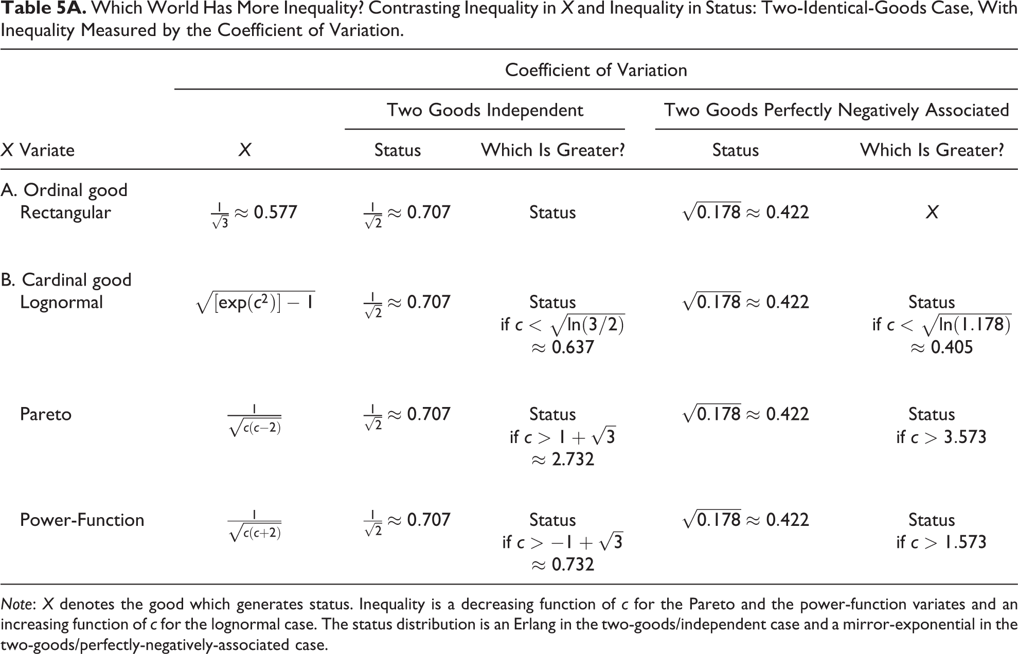
Note: X denotes the good which generates status. Inequality is a decreasing function of c for the Pareto and the power-function variates and an increasing function of c for the lognormal case. The status distribution is an Erlang in the two-goods/independent case and a mirror-exponential in the two-goods/perfectly-negatively-associated case.

Table 5B.

Which World Has More Inequality? Contrasting Inequality in X and Inequality in Status: Two-Identical-Goods Case, With Inequality Measured by the Gini Coefficient.

X Variate	Gini Coefficient
		Two Goods Independent		Two Goods Perfectly Negatively Associated
	X	Status	Which Is Greater?	Status	Which Is Greater?
A. Ordinal good
Rectangular	$\frac{1}{3} \approx 0.333$	.375	Status	$ln (2) - 1 / 2$ ≈ 0.193	X
B. Cardinal good
Lognormal	$2 F_{N} (\frac{c}{\sqrt{2}}) - 1$	.375	Statusif $c < \sqrt{2} Q_{N} (1.375 / 2)$ ≈ 0.691	$ln (2) - 1 / 2$ ≈ 0.193	Statusif $c < \sqrt{2} Q_{N} (1 / 4 + ln \sqrt{2})$ ≈ 0.346
Pareto	$\frac{1}{2 c - 1}$	.375	Statusif $c > 11 / 6$ ≈ 1.833	$ln (2) - 1 / 2$ ≈ 0.193	Statusif $c > 3.089$
Power-Function	$\frac{1}{2 c + 1}$	.375	Statusif $c > 5 / 6$ ≈ .0833	$ln (2) - 1 / 2$ ≈ 0.193	Statusif $c > 2.089$

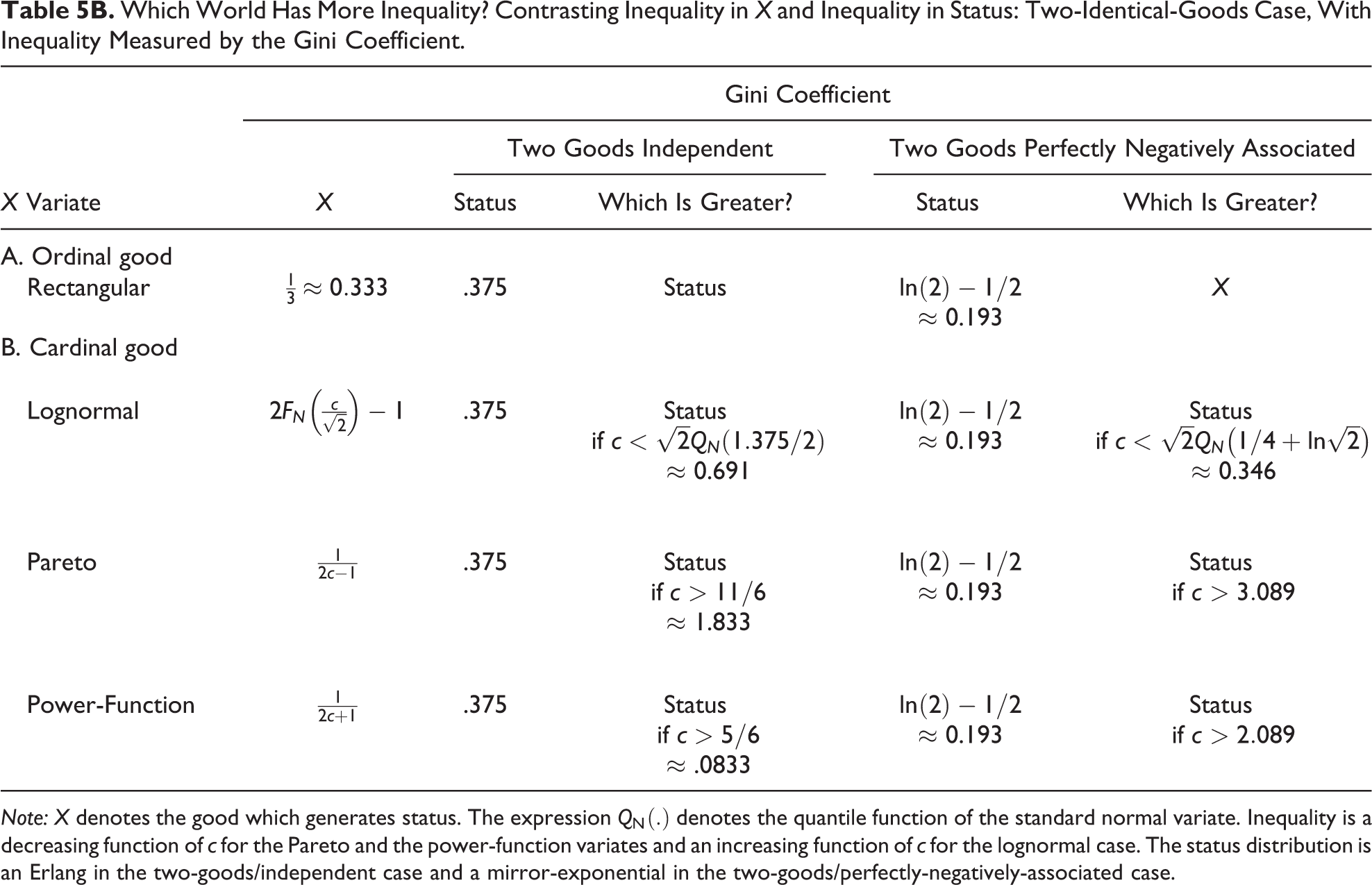
Note: X denotes the good which generates status. The expression $Q_{N} (.)$ denotes the quantile function of the standard normal variate. Inequality is a decreasing function of c for the Pareto and the power-function variates and an increasing function of c for the lognormal case. The status distribution is an Erlang in the two-goods/independent case and a mirror-exponential in the two-goods/perfectly-negatively-associated case.

The first result is thus that inequality across the two worlds can switch direction. When status is the active PSO and the valued goods are ordinal, if the valued goods are one, or two perfectly positively associated goods, or two independent goods, there is more inequality in the second world than in the first world (Tables 4, 5A, and 5B). But if the two ordinal goods are perfectly negatively associated, there is more inequality in the first world than in the second world.

The case of two identical cardinal goods

When the valued goods are cardinal, whether the first world or the second world has more inequality depends on the exact inequality in the cardinal goods’ distribution. Of course, it is more likely that the first world has more inequality if there are two valued goods and they are independent or negatively associated. The rows for the cardinal goods in Tables 5A and 5B show how low the good’s inequality has to be in order for status inequality to be larger. To illustrate, consider a Pareto distributed cardinal good. Its magnitude of the general inequality parameter c need only exceed 1.5 for the single-good status Gini to be larger, but its magnitude must exceed 1.833 for the two-independent-good status Gini to be larger and must exceed 3.089 for the two-perfectly-negatively-associated-goods status Gini to be larger (Tables 4 and 5B). Similar results hold for the coefficient of variation.

To illustrate further, consider a lognormal good. If only one good is valued, the Gini coefficient in the status distribution is .5, and it is larger than the Ginis for lognormals with a general inequality parameter c less than approximately .954 (Table 4). But when two independent and identical goods are valued (Table 5B), the status Gini declines to .375, and it exceeds Ginis for lognormals with a value of c less than approximately .691. And if the two goods are perfectly negatively associated, the status Gini declines to .193, which exceeds Ginis for lognormals with a value of c less than approximately .346. Thus, if the valued goods are lognormal with a value of c equal to .5, there is more inequality in the second world unless the two valued goods are perfectly negatively associated.

Inequality contrasts involving the multiple-identical-good status PSO world

Two natural questions arise: First, how many independent goods must be valued in order for the status Gini coefficient to be lower than an ordinal good’s Gini? Second, at what values of the cardinal goods’ inequality does the status Gini coefficient equal the cardinal good’s Gini? To address these questions, we use the well-known formula for the Gini coefficient in the Erlang distribution (Kleiber and Kotz 2003:164; McDonald and Jensen 1979:856):

G = \frac{Γ (g + 1 / 2)}{Γ (g + 1) \sqrt{π}},

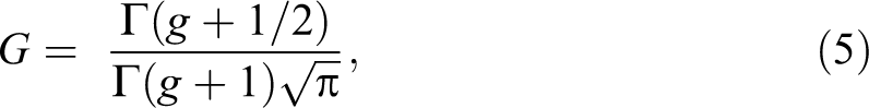
where g denotes the number of goods.

Table 6 reports the Gini coefficient in the status distribution for up to 12 independent valued goods. As is well known, the Gini coefficient in the independent-goods case diminishes quickly, from .5 in the single-good case to .375 in the two-good case, .3125 in the three-good case, and so on. Taking the limits establishes that the Gini coefficient approaches zero as g → ∞.

Table 6.

Gini Coefficient in Two Worlds—The First World and the Status World: Identical and Independent Valued Goods.

Status		General Inequality Parameter c When Variate’s Gini Equals Status Gini
Number of Independent Goods	Gini Coefficient	Lognormal	Pareto	Power-Function
1	.5	.954	1.5	0.5
2	.375	.691	1.833	0.833
3	.3125	.569	2.100	1.100
4	.273	.495	2.329	1.329
5	.246	.443	2.532	1.532
6	.226	.405	2.716	1.716
7	.209	.376	2.887	1.887
8	.196	.352	3.046	2.046
9	.185	.332	3.196	2.196
10	.176	.315	3.338	2.338
11	.168	.300	3.473	2.473
12	.161	.288	3.602	2.602

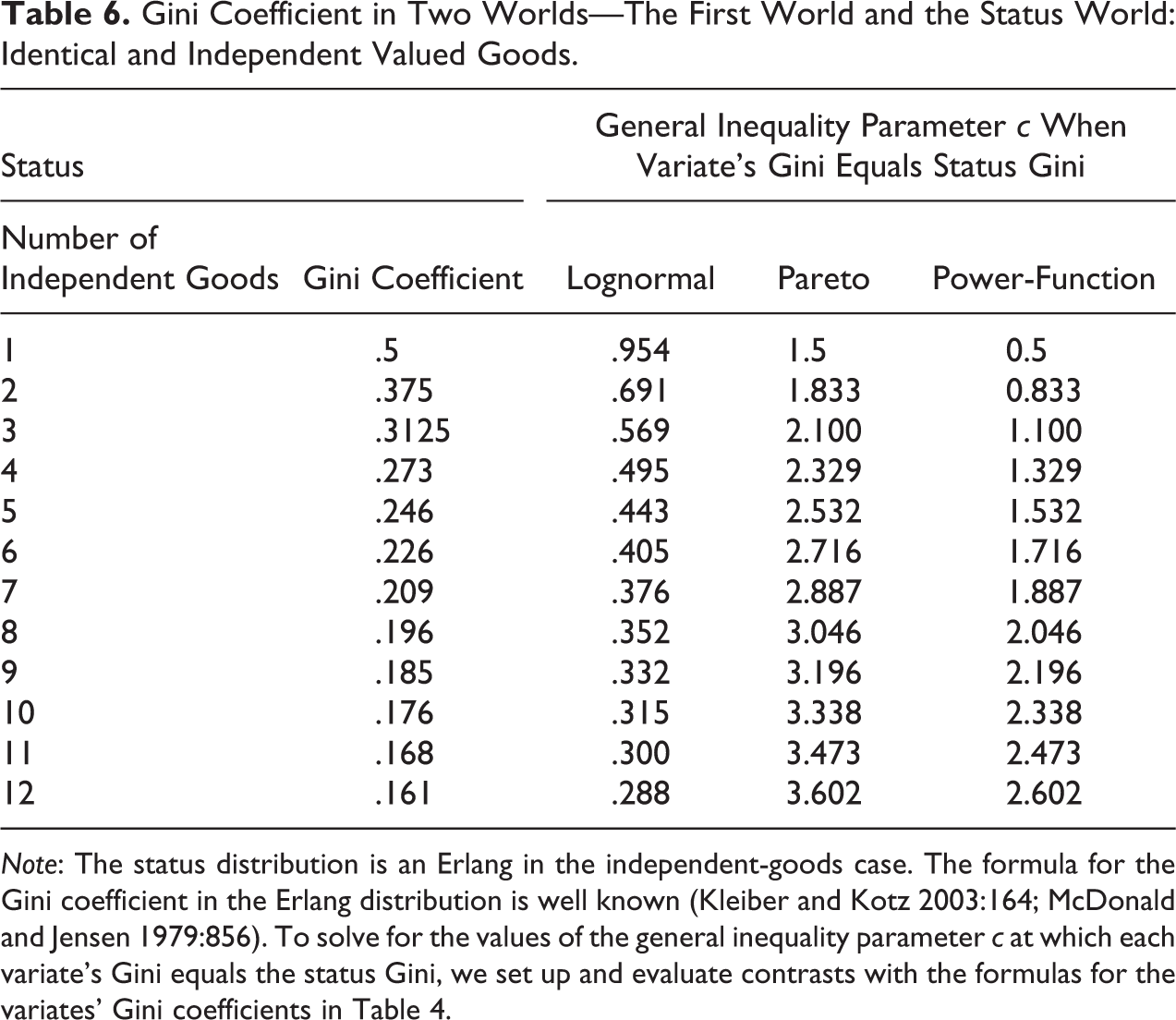
Note: The status distribution is an Erlang in the independent-goods case. The formula for the Gini coefficient in the Erlang distribution is well known (Kleiber and Kotz 2003:164; McDonald and Jensen 1979:856). To solve for the values of the general inequality parameter c at which each variate’s Gini equals the status Gini, we set up and evaluate contrasts with the formulas for the variates’ Gini coefficients in Table 4.

The case of multiple ordinal goods

The ordinal good’s Gini is 1/3, which is less than the status Gini in the two-independent-goods case (.375) but more than in the three-independent-goods case (.3125). Thus, the answer to the question how many independent goods are required in order for the status Gini to be lower than the ordinal good’s Gini is 3. If the same question is addressed using the coefficient of variation, it turns out that the ordinal good’s coefficient of variation is exactly equal to the coefficient of variation in status when there are three independent valued goods, namely, $1 / \sqrt{3}$ . Thus, when inequality is measured by the coefficient of variation, the answer to the question how many independent goods are required in order for status inequality to be lower than the ordinal good’s inequality is 4.

The case of multiple identical cardinal goods

To assess contrasts between status inequality in the multiple-independent-goods case and inequality in cardinal goods (and thus extend Table 5B), Table 6 reports, for each value of the Gini coefficient corresponding to the number of independent goods, the value of the general inequality parameter c in the lognormal, Pareto, and power-function variates when these variates’ Gini coefficient equals the status Gini. To solve for the values of the general inequality parameter c at which each variate’s Gini equals the status Gini, we set up and evaluate contrasts with the formulas for the variates’ Ginis in Table 4. For example, when the number of valued independent goods is 4, the status Gini is .273. This value of Gini is obtained when the lognormal, Pareto, and power-function variates have values of c equal to 0.495, 2.329, and 1.329, respectively.

To visualize these relationships between inequality in the two worlds, Figure 3 provides graphs of the Gini in each of the three modeling variates as a function of the general inequality parameter c (panels A, B, and C), together with the graph of the status Gini as a function of the number of valued independent goods (panel D). Together, Table 6 and Figure 3 aid in visualizing the connection between inequality in the two worlds.

Figure 3.

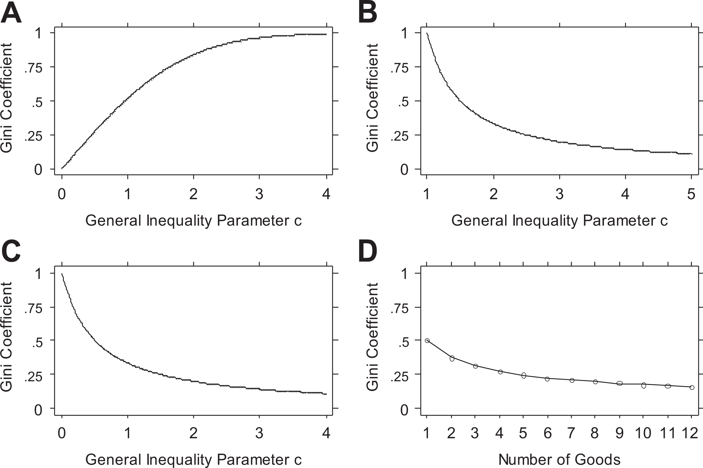
Gini coefficient in three cardinal-good distributions and in the multiple-independent-goods status distribution. (A) Lognormal. (B) Pareto. (C) Power-Function. (D) Status.

Under What Conditions, and by What Mechanisms, Does Inequality in the First World Affect Inequality in the Second World?

The analyses reported in the preceding sections show that there is no single necessary connection between inequality in the first world and inequality in the second world. They can be both zero, both nonzero, or one zero and the other nonzero. If we construct two binary variables for whether inequality in each world is zero or nonzero, their crossclassification yields a table with all four cells populated. All combinations are possible.

Moreover, when both worlds have nonzero inequality, the two magnitudes of inequality may be unrelated. If related, the relation between first-world and second-world inequality may be linear or nonlinear and, if nonlinear, concave or convex. This section presents a few illustrative cases.²⁵

Zero Relation Between Inequality in the Two Worlds

Zero inequality in the first world, nonzero in the second world

The combination of zero inequality in the first world and nonzero in the second world arises in both the case of a single valued good and the case of multiple valued goods.

Zero inequality in the first world, nonzero in the second world: Single valued good

This situation was discussed in the subsections on Deriving the PSO Distribution in the Single-Good Case and Single Valued Good: Distribution-Independent Results. It arises when the single valued good is perfectly equally distributed, justice is the active PSO, and the just amount, X*, varies, reflecting meritocratic ideas of justice. People may find it unjust that everyone is paid the same even though they may differ in reward-relevant characteristics, such as performance or experience. In this case, there is inequality in the second world but not in the first world. As noted above, first-world economic equality is unstable, vulnerable to efforts to achieve justice by introducing inequality.

Zero economic inequality in the first world, nonzero inequality in the second world: Multiple valued goods

Consider again the case where the wage is equal. But suppose now that the PSO is status or power, the valued goods also include beauty and dancing skill, and these two goods vary across people. In this case, the PSO outcome may also vary (or not, depending on the goods’ correlation and the PSO).

Interestingly, in this case, wage equality is not unstable, as in the previous case. Moreover, individuals have the choice of dwelling on the economic equality of the first world or the other inequalities of the first world or the inequality of the second world.

Nonzero inequality in the first world, zero in the second world

Nonzero inequality in the first world, zero in the second world: Single valued good

As seen in the subsections on Deriving the PSO Distribution in the Single-Good Case and Single Valued Good: Distribution-Independent Results, as well as Table 3, when the active PSO is justice and both X and X* vary, if X and X* are identical and perfectly positively associated, then the PSO outcome is the same for everyone (zero, the point of perfect justice), and there is no inequality. No matter how much or in what direction income inequality may change, justice inequality will remain zero.

As noted above, in this case, where the first world has inequality but the second world does not, the second world provides refuge, and with it a casual accommodation with economic inequality that can retard or inhibit efforts to reduce it.

Nonzero inequality in the first world, zero in the second world: Multiple valued goods

As reported above, starting in the subsection on How to Change Inequality in the Second World, there are several configurations of multiple goods—such as the case of two identical goods perfectly negatively correlated—in which the PSO outcome is zero for everyone.

Nonzero inequality in the first world, constant inequality in the second world

The inequality measures reported in the fourth section indicate that inequality in the second world can be constant and hence completely unresponsive to inequality in the first world. Second-world inequality that is constant (and nonzero) arises in two cases: (1) when the active PSO is status, and (2) when the valued good is either ordinal or else a cardinal good treated ordinally—as depicted in the T formation of Table 2 and the T’s stem of Figures 2A and 2B. In these cases, the inequality in the first world is irrelevant to the inequality in the second world.

To illustrate, if status is the active PSO and the valued good is income, then no matter how much or in what direction income inequality changes, status inequality remains the same.

Nonzero Relation Between Inequality in the Two Worlds

Nonzero relation between inequality in the two worlds: Single valued good

Second-world inequality governed by first-world inequality

Look again at Table 2 and Figures 2A and 2B, focusing on the cases where the active PSO is justice or power, the (single) valued good is cardinal, and, in the justice case, the comparison standard (or just reward) is constant (viz., the cases outside the T). The formulas in Table 2 and the graphs in Figures 2A and 2B depict inequality in the second world—inequality in the justice and power PSO distributions, represented by the variance and the GMD—as a function of the general inequality parameter c in the possessions of the first world. As shown, the relation is monotonic in all 12 formulas and the corresponding 12 graphs. Thus, in these cases, inequality in the second world is clearly and unambiguously governed by inequality in the first world.

Power PSO inequality a linear function of first-world inequality

Recall now that the power PSO, shown in equation (3), is a linear function of the cardinal good X. Thus, inequality in the power PSO distribution will vary linearly with inequality in the cardinal good. To see this, compare the formulas for the variance and the GMD of X and of P. The formulas for Var(P) and GMD(P) are in Table 2. The formulas for Var(X) and GMD(X) can be obtained from the formulas for the Gini coefficient and the coefficient of variation (used earlier and widely available, e.g., in Jasso 2018:201).²⁶

Justice PSO inequality a nonlinear function of first-world inequality

To assess the effect of first-world inequality on second-world inequality in the justice PSO case, we compare the variance and GMD of X and Z. Table 7 assembles the variances for the cardinal goods and for the justice PSO, when the comparison amount is a constant (from Table 2). For simplicity, the good’s mean is set at unity. As in Table 2, both Var(X) and Var(Z) are expressed as functions of the good’s general inequality parameter c.²⁷

Table 7.

Relation Between the Variance in the First World and the Variance in the Second World: Two Cases Where the Justice PSO Is Generated by (1) a Single Cardinal Good and (2) Two Independent and Equally Weighted Goods, One Cardinal, the Other Ordinal.

X VariateA Cardinal Good	Var(X)	Justice PSO
		Single Valued GoodA Cardinal Good		Two Valued GoodsOne Cardinal, the Other Ordinal
		Var(Z)		Var(T)
		Expressed as a Function of c	Expressed as a Function of Var(X)	Expressed as a Function of c	Expressed as a Function of Var(X)
Lognormal	$exp (c^{2}) - 1$	c²	$ln [1 + Var (X)]$	$\frac{c^{2} + 1}{4}$	$\frac{1 + ln [1 + Var (X)]}{4}$
Pareto	$\frac{1}{c (c - 2)}$	$\frac{1}{c^{2}}$	—	$\frac{c^{2} + 1}{4 c^{2}}$	—
Power-Function	$\frac{1}{c (c + 2)}$	$\frac{1}{c^{2}}$	—	$\frac{c^{2} + 1}{4 c^{2}}$	—

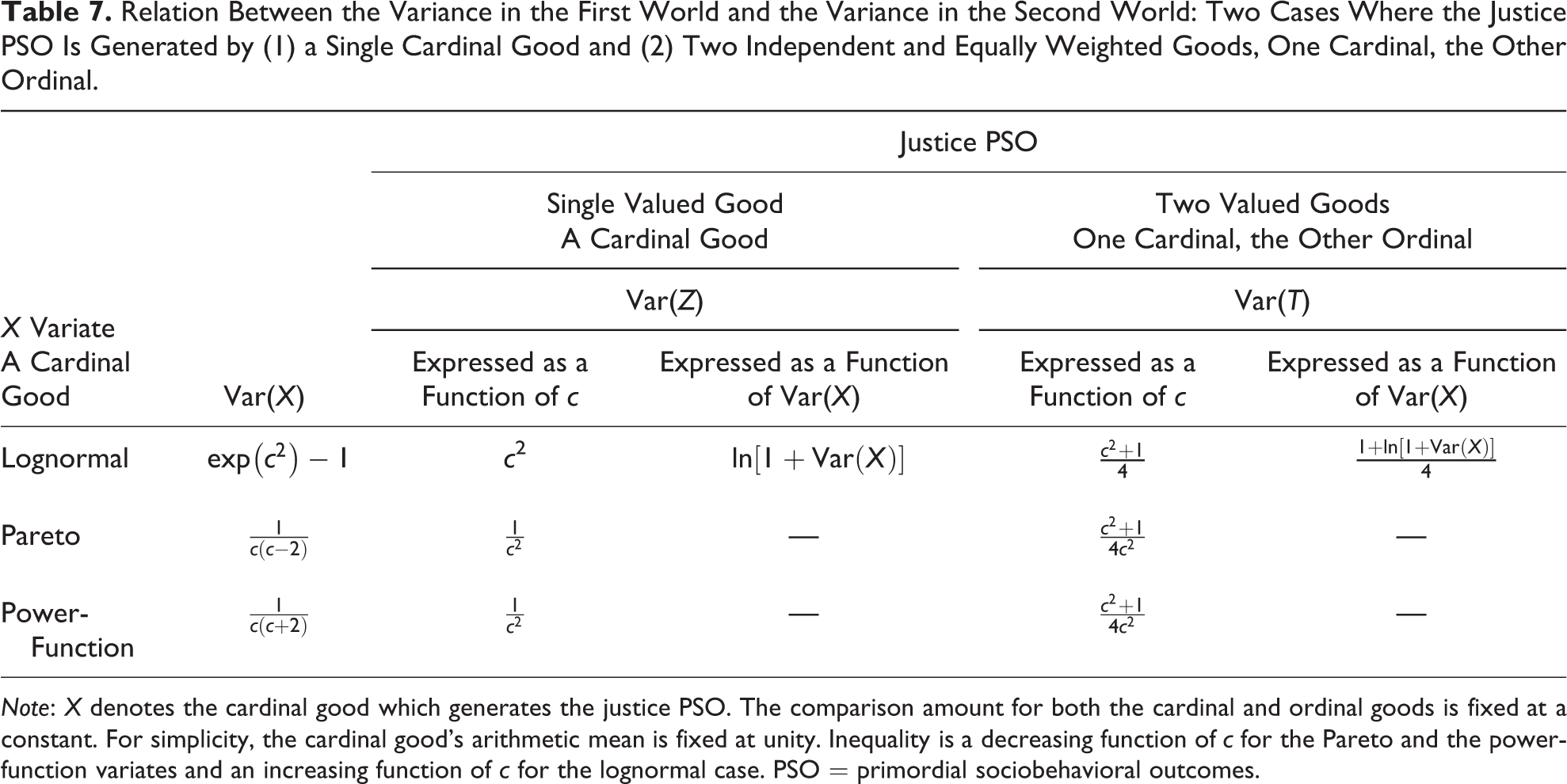
Note: X denotes the cardinal good which generates the justice PSO. The comparison amount for both the cardinal and ordinal goods is fixed at a constant. For simplicity, the cardinal good’s arithmetic mean is fixed at unity. Inequality is a decreasing function of c for the Pareto and the power-function variates and an increasing function of c for the lognormal case. PSO = primordial sociobehavioral outcomes.

It would be useful to derive expressions for the variance of the justice PSO as a function of the variance in X, but that is straightforward only for the lognormal variate. In the lognormal case, algebraic manipulation, setting the good’s mean to unity, leads quickly to the expression:

Var (Z) = ln [1 + Var (X)] .

This formula is incorporated into Table 7 (fourth column). In this pristine case, inequality in the second world is a logarithmic function of inequality in the first world.

To visualize the associations between the variance of X and the variance of the justice PSO in all three variates, we show in Figure 4 graphs of Var(Z) on Var(X). To contrast these associations with a linear association, the grids also include the diagonal. As shown, the associations are highly nonlinear. All three curves depart substantially from the diagonal. The association is downwardly concave in the lognormal (as expected from the formula) and Pareto and upwardly concave in the power-function. In the Pareto, an association is almost nonexistent in the ranges depicted in the graph, Var(Z) ranging from .04 to .22 as Var(X) ranges from 0 to 4.

Figure 4.

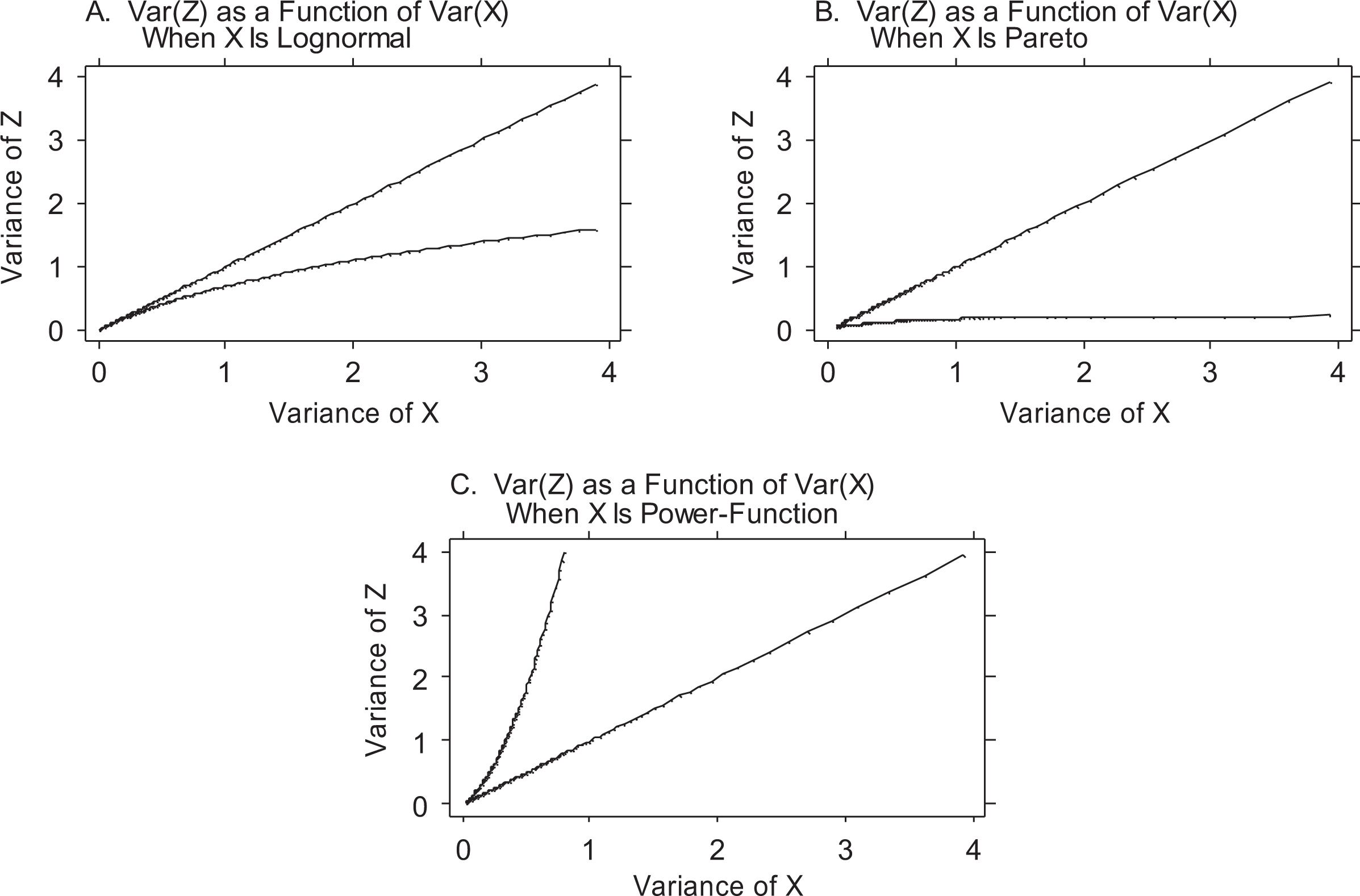
Variance in the justice PSO distribution arising from a single valued cardinal good, expressed as a function of the variance in the cardinal good, with the cardinal goods modeled by three variates. The diagonals enable visualizing the nonlinearity of the relation between Var(X) and Var(Z). (A) Var(Z) as a function of Var(X) when X is lognormal. (B) Var(Z) as a function of Var(X) when X is Pareto. (C) Var(Z) as a function of Var(X) when X is power-function.

A similar exercise using the GMD instead of the variance again yields nonlinearities but with different convexity patterns. The association between inequality in the first world and inequality in the second world is highly nonlinear in all three variates. It is upwardly concave in the lognormal and power-function and downwardly concave in the Pareto.

Thus, in cases where the outcome in the second world is generated by a single good in the first world, the association between inequality in the first world and inequality in the second world can be nonexistent, linear, or nonlinear, and, in the latter case, the character of the nonlinearity depends on the particular measure of inequality.

Nonzero relation between inequality in the two worlds: Multiple valued goods

The relation between inequality in each good in the first world and inequality in the corresponding single-good PSO distribution remains intact and exactly as already described. However, the relation between each good’s inequality and inequality in the multiple-good PSO distribution depends on all the good-specific relations and may become complicated.

The case of identical and perfectly positively associated PSO distributions

Recall from the subsection on Deriving the PSO Distribution in the Multiple-Good Case the distribution-independent result that in the case of identical PSO distributions which are perfectly positively associated, the multiple-good PSO distribution remains the same. Thus, the variance of the multiple-good PSO distribution is the same as the variance in the single-good PSO distributions. Accordingly, any results already established for the relation between the variance of X and the variance of the single-good PSO extend to this case. For example, the associations depicted in Figure 4 hold as well when the multiple-good PSO distribution is the average of identical, perfectly positively associated, single-good PSO distributions.

Justice PSO inequality a nonlinear function of first-world economic inequality in the case of two independent goods, one cardinal and one ordinal

Next, we analyze the case where justice is the active PSO and two independent goods, one cardinal and the other ordinal, are equally valued. As in equation (4) in the subsections on The Multiple-Input Primordial Sociobehavioral Outcome and How to Change Inequality in the Second World, let T denote a multiple-good PSO distribution such as this two-goods-independent justice PSO distribution. In the general distribution-independent case, its variance, denoted Var(T), is the classic weighted sum of the component variances. In the special case of one ordinal good and one cardinal good, the formula for the variance can be expressed:

Var (Z) = \frac{Var (Z_{ord}) + Var (Z_{card})}{4} .

Thus, the variance of this two-goods-independent justice PSO distribution is a linear function of the variances of the single-good justice PSO distributions.

Using the result from Table 2 that the variance of the justice PSO arising from an ordinal good is one, the variance of this two-goods-independent justice PSO distribution reduces to:

Var (T) = \frac{1 + Var (Z_{card})}{4} .

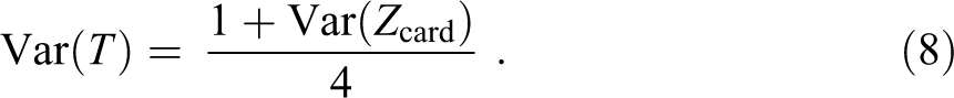
It is then straightforward to obtain the variances Var(Y) for the three cases in which the cardinal good is lognormal, Pareto, and power-function by plugging into formula (8) the corresponding variance of the single-good justice PSO distribution (from Table 2 or Table 7). Accordingly, when the cardinal good is lognormal, the variance is (c² + 1)/4. When the cardinal good is either Pareto or power-function, the final variance is (c² + 1)/(4c²). These variances of the final two-goods-independent justice PSO distribution are expressed as functions of the cardinal good’s general inequality parameter c and collected in Table 7 (fifth column).

As before, it would be useful to obtain expressions for the variance of the justice PSO as a function of the variance in the cardinal good, but, again as before, that is straightforward only for the lognormal variate. In the lognormal case, using formulas (6) and (8) quickly yields the formula for Var(T) as a function of Var(X):

Var (T) = \frac{1 + ln [1 + Var (X)]}{4} .

Of course, given the general expression for the variance in equation (8), it is no surprise that formula (9) for the two-goods-independent case is a linear function of formula (6) for the single-good case. Formula (9) completes the summary in Table 7 (sixth column).

Again as before, the lack of analytic expressions for Var(T) as a function of Var(X) in the Pareto and power-function cases is no bar to visualizing this relation. Figure 5 depicts graphs of the variance in the final two-good justice PSO distributions described above, as a function of the variance in the cardinal good. As shown, the relation is nonlinear and of opposite convexity in the lognormal and power-function cases, while in the Pareto case, the relation, though nonlinear and downwardly concave, is so weak in the range depicted in the graph that to the naked eye it appears almost null.

Figure 5.

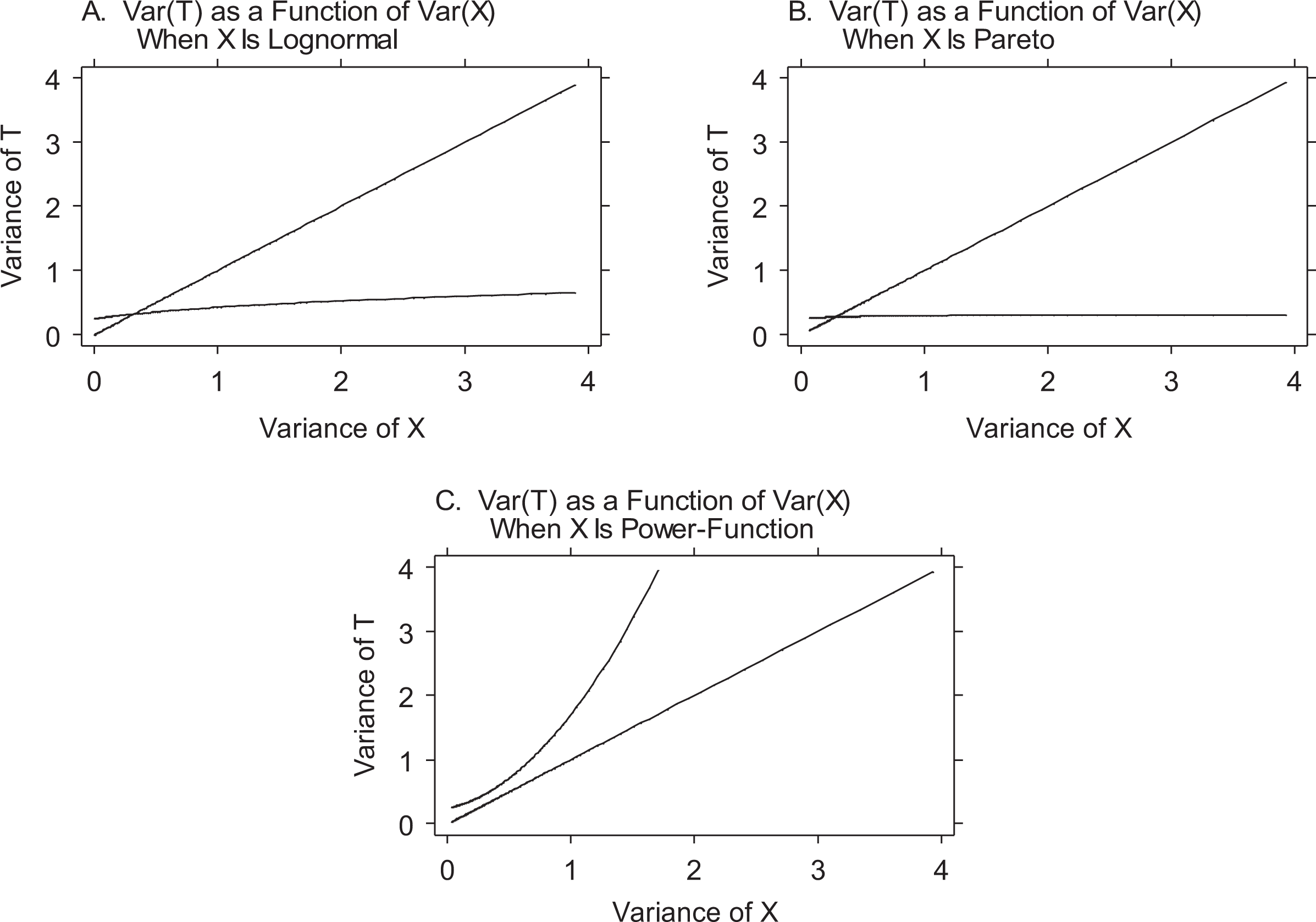
Variance in the justice PSO distribution arising from two independent and equally weighted valued goods, one ordinal and the other cardinal, expressed as a function of the variance in the cardinal good, with the cardinal goods modeled by three variates. The diagonals enable visualizing the nonlinearity of the relation between Var(X) and Var(Z). (A) Var(Y) as a function of Var(X) when X is lognormal. (B) Var(Y) as a function of Var(X) when X is Pareto. (C) Var(Y) as a function of Var(X) when X is power-function.

As expected, the graphs in Figures 4 and 5 are very similar. Figure 4 depicts the graphs of Var(Z) as a function of Var(X), and Figure 5 depicts the graphs of Var(T)—a linear function of Var(Z)—as a function of Var(X).²⁸

Concluding Note

Inequality often appears in linked pairs of inputs and outcomes, such as schooling and income, income and consumption, and wealth and happiness, and Veblen’s ([1899] 1953) famous observation, “Wealth confers honor.” Understanding inequality requires understanding input inequality, outcome inequality, and the relation between the two—in both inequality between persons and inequality between subgroups. This article contributes to the methodological toolkit for studying inequality by developing a framework that makes explicit both input inequality and outcome inequality and by addressing three main associated questions:

How do the mechanisms for generating and altering inequality differ across inputs and outcomes?

Which have more inequality—inputs or outcomes?

Under what conditions, and by what mechanisms, does input inequality affect outcome inequality?

The key to the framework is the twofold idea (1) that there is a special relation between input and outcome and (2) that input and outcome each have a distribution. Thus, for example, if we know the special relation—the function connecting input and outcome—and if we know the distribution of the input, we can obtain the distribution of the outcome. And from the input distribution and the outcome distribution, we obtain the input inequality and the outcome inequality—and connect them.

Given the abundance of inputs, input–outcome functions, and input distributions, and for simplicity and concreteness, in this first foray, we provided a theory-based application with a starter set of three types of input-outcome relations and four input distributions. The theory focuses on personal quantitative characteristics (like beauty or wealth) and the major sociobehavioral outcomes (like justice or status) they generate.

Results include the following: First, under specified conditions, distinctive mechanisms govern inequality in inputs and inequality in outcomes. Second, input inequality and outcome inequality can be the same or different; if different, whether inequality is greater among inputs or outcomes depends on the configuration of outcome function, types of inputs, distributional form of and inequality in cardinal inputs, and number of and associations among the inputs. Third, the link between input inequality and outcome inequality is multiform; it can be nonexistent, linear, or nonlinear, and if nonlinear, it can be concave or convex.

More deeply, this work signals the formidable empirical challenges in studying inequality but also the fast growing toolbox. For example, even if the outcome distribution is difficult to derive, fundamental theorems on the variance make it possible to analyze the input–outcome inequality connection. Similarly, within specified distributions, the general inequality parameter makes it possible to express results in terms of both measures of overall inequality and measures of subgroup inequality.

Even at this early stage, this work on the input–outcome inequality connection already sheds light on aspects of what Darity and Deshpande (2000:77) call the “deep structure” of inequality, in particular, the disjuncture between economic inequality and experienced inequality, the fragility of economic equality, and the blissful obliviousness to economic inequality.

But much work remains to be done. Theoretically, it would be useful to analyze a variety of further nonlinear input–outcome functions and further input distributions. Empirically, it would be useful to examine a variety of inputs and outcomes in representative samples across countries and over time, including long chains of inputs and outcomes.

Supplemental Material

Supplemental Material, sj-pdf-1-smr-10.1177_00491241211014245 - Linking Input Inequality and Outcome Inequality

Supplemental Material, sj-pdf-1-smr-10.1177_00491241211014245 for Linking Input Inequality and Outcome Inequality by Guillermina Jasso in Sociological Methods & Research

Footnotes

Author’s Note

Earlier versions of portions of this article were presented at the Annual Winter Meeting of the Methodology Section of the American Sociological Association, Urbana, IL, April 2010; at the Group Processes Conference, Atlanta, GA, August 2010; at New York University, October 2010; at the University of Pennsylvania, March 2011; at the Otto Friedrich University, Bamberg, Germany, October 2011; at the University of Cologne, December 2012; at the University of Cambridge, United Kingdom, May 2014; at the Karl F. Schuessler Lecture in the Methodologies of Social Research at Indiana University, Bloomington, April 2016; at the Summer Institute on the Empirical Implications of Theoretical Models (EITM), sponsored by the Hobby School of Public Affairs, University of Houston, Houston, TX, June 2017; at the Annual Meeting of the American Sociological Association, Montreal, Canada, August 2017; at the 11th Conference of the International Network of Analytical Sociologists (INAS), Stanford University, June 2018; at the Joint Statistical Meetings, Vancouver, Canada, July-August 2018; at the Annual Meeting of the American Sociological Association, Philadelphia, PA, August 2018; and at the Eighth Meeting of the Society for the Study of Economic Inequality (ECINEQ), Paris, France, July 2019.

Acknowledgments

I thank conference participants, James S. Granato, Jerry Lynn Johnson, Jr., Tim F. Liao, J. Scott Long, Eva Meyersson Milgrom, Frank P. Scioli, Hawal Shamon, the anonymous referees, and the editor for valuable comments and suggestions. I also gratefully acknowledge the intellectual and financial support of New York University.

Declaration of Conflicting Interests

The author(s) declared no potential conflicts of interest with respect to the research, authorship, and/or publication of this article.

Funding

The author(s) received no financial support for the research, authorship, and/or publication of this article.

ORCID iD

Guillermina Jasso

Supplemental Material

The supplemental material for this article is available online.

Notes

References

Abramitzky

Ran

. 2018. The Mystery of the Kibbutz: Egalitarian Principles in a Capitalist World. Princeton, NJ: Princeton University Press.

Adams

J. Stacy

. 1963. “Toward an Understanding of Inequity.” Journal of Abnormal and Social Psychology 67:422–36.

Adams

J. Stacy

. 1965. “Inequity in Social Exchange.” Pp. 267–99 in Advances in Experimental Social Psychology, Vol. 2, edited by Berkowitz

Leonard

. New York: Academic Press.

Agresti

Alan

Finlay

Barbara

. 2009. Statistical Methods for the Social Sciences. 4th ed. Upper Saddle River, NJ: Pearson Prentice Hall.

Allen

R. G. D.

1938. Mathematical Analysis for Economists. New York: St. Martin’s Press.

Ashenfelter

Orley

Levine

Phillip B.

Zimmerman

David J.

. 2003. Statistics and Econometrics: Methods and Applications. New York: Wiley.

Atkinson

Anthony B.

1970. “On the Measurement of Inequality.” Journal of Economic Theory 2:244–63.

Bales

Robert F.

Strodtbeck

Fred L.

Mills

Theodore M.

Roseborough

Mary E.

. 1951. “Channels of Communication in Small Groups.” American Sociological Review 16:461–68.

Berger

Joseph

Cohen

Bernard P.

Zelditch

Morris

Jr . 1966. “Status Characteristics and Expectation States.” Pp. 29–46 in Sociological Theories in Progress, Vol. 1, edited by Berger

Joseph

Zelditch

Morris

Jr Bo

Anderson

. Boston, Boston, MA: Houghton Mifflin.

10.

Berger

Joseph

Zelditch

Morris

Jr Anderson

Cohen

Bernard P.

. 1972. “Structural Aspects of Distributive Justice: A Status Value Formulation.” Pp. 119–146 in Sociological Theories in Progress, Vol. 2, edited by Berger

Joseph

Zelditch

Morris

Jr Anderson

. Boston, MA: Houghton Mifflin.

11.

Berger

Joseph

Hamit Fisek

Norman

Robert Z.

Zelditch

Morris

Jr . 1977. Status Characteristics and Social Interaction. New York: Elsevier.

12.

Berger

Joseph

Rosenholtz

Susan J.

Zelditch

Morris

Jr . 1980. “Status Organizing Processes.” Annual Review of Sociology 6:479–508.

13.

Bernoulli

Daniel

. [1738] 1954. “Exposition of a New Theory on the Measurement of Risk.” Econometrica 22:23–36. Translated by

Sommer

14.

Blau

Peter M.

1964. Exchange and Power in Social Life. New York: Wiley.

15.

Blau

Peter M.

1974. “Presidential Address: Parameters of Social Structure.” American Sociological Review 39:615–35.

16.

Brown

Roger

. 1986. Social Psychology: The Second Edition. New York: Free Press.

17.

Clogg

Clifford C.

1992. “The Impact of Sociological Methodology on Statistical Methodology.” Statistical Science 7:183–96.

18.

Cowell

Frank A.

1977. Measuring Inequality: Techniques for the Social Sciences. New York: Wiley Halsted.

19.

Cowell

Frank A.

2011. Measuring Inequality. 3rd ed. Oxford, England: Oxford University Press.

20.

Cramer

J. S.

1971. Empirical Econometrics. Amsterdam, the Netherlands: North-Holland.

21.

Dagum

Camilo

. 1983. “Income Inequality Measures.” Pp. 34–40 in Encyclopedia of Statistical Sciences, Vol. 4, edited by Kotz

Samuel

Johnson

Norman L.

Read

Campbell B.

. New York: Wiley.

22.

Darity

William A.

Jr. Deshpande

Ashwini

. 2000. “Tracing the Divide: Intergroup Disparity across Countries.” Eastern Economic Journal 26:75–85.

23.

Diekmann

Andreas

. 2004. “The Power of Reciprocity: Fairness, Reciprocity, and Stakes in Variants of the Dictator Game.” Journal of Conflict Resolution 48:487–505.

24.

Dowd

Maureen

. 2014. “Isn’t It Rich?” New York Times, July 13, p. SR11.

25.

Epictetus. 1983. Handbook of Epictetus. Translated, with introduction and annotations, by Nicholas White. Indianapolis, IN: Hackett. Based on the lectures of Epictetus, who lived circa 50–130 A.D.

26.

Estlund

David M.

2009. Democratic Authority: A Philosophical Framework. Princeton, NJ: Princeton University Press.

27.

Evans

M. D. R.

Kelley

Jonathan

Peoples

Clayton D.

. 2010. “Justifications of Inequality: The Normative Basis of Pay Differentials in 31 Nations.” Social Science Quarterly 91:1405–31.

28.

Fechner

Gustav T.

1860. Elemente der Psychopysik. Leipzig, Germany: Breitkopf & Härtel.

29.

Fechner

Gustav T.

1877. In Sachen der Psychophysik. Leipzig, Germany: Breitkopf & Härtel.

30.

Forbes

Catherine

Evans

Merran

Hastings

Nicholas

Peacock

Brian

. 2011. Statistical Distributions. 4th ed. New York: Wiley.

31.

Freedman

David

Pisani

Robert

Purves

Roger

. [1978] 1998. Statistics. 3rd ed. New York: W. W. Norton.

32.

Friedman

Milton

. 1977. “Fair versus Free.” Newsweek, July 4, p. 70. Originally delivered as a commencement address at Virginia Polytechnic Institute, May 28, 1977.

33.

Gabaix

Xavier

. 2016. “Power Laws in Economics: An Introduction.” Journal of Economic Perspectives 30(1):185–206.

34.

Galton

Francis

. 1899. Natural Inheritance. London, England: Macmillan.

35.

Gastwirth

Joseph L.

1972. “The Estimation of the Lorenz Curve and Gini Index.” The Review of Economics and Statistics 54:306–16.

36.

Gill

Jeff

. 2006. Essential Mathematics for Political and Social Research. Cambridge, England: Cambridge University Press.

37.

Gini

Corrado

. 1914. “Sulla Missura della Concentrazione e della Variabilità dei Caratteri.” Atti del Reale Istituto Veneto di Scienze, Lettere ed Arti 73:1203–48.

38.

Goode

William J.

1978. The Celebration of Heroes: Prestige as a Control System. Berkeley: University of California Press.

39.

Hoel

Paul G

. [1947] 1971. Introduction to Mathematical Statistics. 4th ed. New York: Wiley.

40.

Homans

George C.

1961. Social Behavior: Its Elementary Forms. New York: Harcourt, Brace, Jovanovich.

41.

Homans

George C.

1976. “Commentary.” Pp. 231–44 in Advances in Experimental Social Psychology, Vol. 9, edited by Berkowitz

Walster

. New York: Academic Press.

42.

Hout

Michael

DiPrete

Thomas A.

. 2006. “What We Have Learned: RC28’s Contributions to Knowledge about Social Stratification.” Research in Social Stratification and Mobility 24:1–20.

43.

International Sociological Association. 1981. “The History of the Research Committee on Social Stratification and Social Mobility of the ISA.” Part 1, from 1950 to 1970, written by Natalie Rogoff-Ramsøy; Part II, from 1970 to 1981, written by Walter Müller. Retrieved 7 June 2021. https://sites.google.com/site/rc28hp/about/history.

44.

Jasso

Guillermina

. 1978. “On the Justice of Earnings: A New Specification of the Justice Evaluation Function.” American Journal of Sociology 83:1398–419. doi: 10.1086/226706.

45.

Jasso

Guillermina

. 1980. “A New Theory of Distributive Justice.” American Sociological Review 45:3–32. doi: 10.2307/2095239.

46.

Jasso

Guillermina

. 1990. “Methods for the Theoretical and Empirical Analysis of Comparison Processes.” Sociological Methodology 20:369–419. doi: 10.2307/271091.

47.

Jasso

Guillermina

. 2001. “Studying Status: An Integrated Framework.” American Sociological Review 66(1):96–124. doi: 10.2307/2657395.

48.

Jasso

Guillermina

. 2008a. “A New Unified Theory of Sociobehavioral Forces.” European Sociological Review 24(4):411–34. doi: 10.1093/esr/jcn023.

49.

Jasso

Guillermina

. 2008b. “The Terms and Relations of Comparison, Referential, and Relative Processes.” Pp. 265–290 in Rational Choice: Theoretische Analyse und Empirische Resultate. Festschrift für Karl-Dieter Opp, edited by Diekmann

Eichner

Schmidt

Voss

. Wiesbaden, Germany: VS Verlag. doi:10.1007/978-3-531-90866-3_15.

50.

Jasso

Guillermina

. 2011. “Migration and Stratification.” Social Science Research 40(5):1292–336. doi: 10.1016/j.ssresearch.2011.03.007.

51.

Jasso

Guillermina

. 2015. “Thinking, Saying, Doing in the World of Distributive Justice.” Social Justice Research 28(4):435–78. doi: 10.1007/s11211-015-0257-3.

52.

Jasso

Guillermina

. 2016. “(In)Equality and (In)Justice.” Civitas—Revista de Ciências Sociais 16(2):189–217. doi: 10.15448/1984-7289.2016.2.23118.

53.

Jasso

Guillermina

. 2017. “Inequality in the Distribution of a Good Is a Bad, and Inequality in the Distribution of a Bad Is a Good.” European Sociological Review 33(4):604–14. https://doi.org/10.1093/esr/jcx062.

54.

Jasso

Guillermina

. 2018. “What Can You and I Do to Reduce Inequality?” Journal of Mathematical Sociology 42(4):186–204. doi: 10.1080/0022250X.2017.1343826.

55.

Jasso

Guillermina

. 2020. “Anything Lorenz Curves Can Do, Top Shares Can Do: Assessing the TopBot Family of Inequality Measures.” Sociological Methods & Research 49(4):947–81. doi: 10.1177/0049124118769106.

56.

Jasso

Guillermina

. 2021. “New Results Linking Inequality and Justice.” Journal of Mathematical Sociology 45(1):1–21. doi: 10.1080/0022250X.2020.1715970.

57.

Jasso

Guillermina

Kotz

Samuel

. 2007. “A New Continuous Distribution and Two New Families of Distributions Based on the Exponential.” Statistica Neerlandica 61(3):305–28. doi: 10.1111/j.1467-9574.2007.00358.x.

58.

Jasso

Guillermina

Kotz

Samuel

. 2008a. “Probability Distributions.” Pp. 491–98 in International Encyclopedia of the Social Sciences, 2nd ed., Vol. 6, edited by Jr

W. A. D.

. Detroit, MI: Macmillan Reference USA.

59.

Jasso

Guillermina

Kotz

Samuel

. 2008b. “Two Types of Inequality: Inequality between Persons and Inequality between Subgroups.” Sociological Methods & Research 37(1):31–74. doi: 10.1111/j.1467-9574.2007.00358.x.

60.

Jasso

Guillermina

Liao

Tim Futing

. 2003. “Distribution.” Pp. 276–80 in The Sage Encyclopedia of Social Science Research Methods, Vol. 1, edited by Lewis-Beck

Michael

Bryman

Alan

Liao

Tim Futing

. Thousand Oaks, CA: Sage Publications. doi: 10.4135/9781412950589.n252.

61.

Jencks

Christopher

Smith

Marshall

Acland

Henry

Bane

Mary Jo

Cohen

David

Gintis

Herbert

Heyns

Barbara

Michelson

Stephan

. 1972. Inequality: A Reassessment of the Effect of Family and Schooling in America. New York: Basic Books.

62.

Johnson

Norman L.

Kemp

Adrienne W.

Kotz

Samuel

. 2005. Univariate Discrete Distributions. 3rd ed. New York: Wiley.

63.

Johnson

Norman L.

Kotz

Samuel

. 1969–1972. Distributions in Statistics. Four volumes. New York: Wiley.

64.

Johnson

Norman L.

Kotz

Samuel

Balakrishnan

. 1994–1995. Continuous Univariate Distributions. Two volumes. New York: Wiley.

65.

Kleiber

Christian

Kotz

Samuel

. 2003. Statistical Size Distributions in Economics and Actuarial Sciences. Hoboken, NJ: Wiley.

66.

Lerner

Melvin J.

1980. The Belief in a Just World: A Fundamental Delusion. New York . Plenum.

67.

Liebig

Stefan

Sauer

Carsten

. 2016. “Sociology of Justice.” Pp. 37–59 in Handbook of Social Justice Theory and Research, edited by Sabbagh

Schmitt

. New York: Springer.

68.

McDonald

James B.

Jensen

Bartell C.

. 1979. “An Analysis of Some Properties of Alternative Measures of Income Inequality Based on the Gamma Distribution Function.” Journal of the American Statistical Association 74:856–60.

69.

McQuarrie

Christopher

Geller

Bruce

. 2018. Mission: Impossible—Fallout. Retrieved 7 June 2021. https://www.imdb.com/title/tt4912910/. https://www.imdb.com/title/tt4912910/quotes.

70.

Merton

Robert K.

1968. Social Theory and Social Structure. Revised and enlarged edition. New York: Free Press.

71.

Pen

Jan

. 1971. Income Distribution. London, England: Allen Lane.

72.

Plato [c. 428–348/7 BC]. 1952. The Dialogues of Plato. Translated by Jowett

Benjamin

. Chicago, IL: Britannica.

73.

Quetelet

Adolphe

. [1835] 1842. A Treatise on Man and the Development of His Faculties. Edinburgh, England: Chambers.

74.

Rayo

Luis

Becker

Gary S.

. 2007. “Evolutionary Efficiency and Happiness.” Journal of Political Economy 115:302–37.

75.

Runciman

William G.

1961. “Problems of Research on Relative Deprivation.” Archives Européennes de Sociologie 2:315–23.

76.

Runciman

William G.

1966. Relative Deprivation and Social Justice. Berkeley: University of California.

77.

Samuelson

Paul

. 1990. “Deterministic Chaos in Economics: An Occurrence in Axiomatic Utility Theory.” Pp. 42–63 in Nonlinear and Multisectoral Macrodynamics, edited by Velupillai

. London, UK: Macmillan.

78.

Semple

Kirk

. 2018. “Virgin of Guadalupe is ‘No. 1 Mother’ in Mexico, a Binding Force across Divides.” New York Times, December 16, p. A9.

79.

Sewell

William H.

Hauser

Robert M.

. 1975. Education, Occupation, and Earnings: Achievement in the Early Career. New York: Academic.

80.

Sørensen

Aage B.

1979. “A Model and a Metric for the Analysis of the Intragenerational Status Attainment Process.” American Journal of Sociology 85:361–84.

81.

Stephan

Frederick F.

1952. “The Relative Rate of Communication between Members of Small Groups.” American Sociological Review 17:482–86.

82.

Stephan

Frederick F.

Mishler

Elliot G.

. 1952. “The Distribution of Participation in Small Groups: An Exponential Approximation.” American Sociological Review 17:598–608.

83.

Stuart

Alan

Keith Ord

. 1987. Kendall’s Advanced Theory of Statistics, Volume 1, Distribution Theory. 5th ed. Originally by Kendall

S. M.

. New York: Oxford University Press.

84.

Theil

Henri

. 1967. Economics and Information Theory. Amsterdam, the Netherlands: North-Holland.

85.

U.S. National Institute of Standards and Technology. 2018. eHandbook of Statistical Methods. Retrieved 7 June 2021. http://www.itl.nist.gov/div898/handbook/.

86.

van der Vaart

H. Robert

. 1968. “Variances, Statistical Study of.” Pp. 292–300 in International Encyclopedia of the Social Sciences, Vol. 16, edited by Sills

D. L.

. New York: Macmillan.

87.

Veblen

Thorstein

. [1899] 1953. The Theory of the Leisure Class: An Economic Study of Institutions. Rev. ed. Reprint, New York: New American Library.

88.

Wagner

David

Berger

Joseph

. 1985. “Do Sociological Theories Grow?” American Journal of Sociology 90:697–728.

89.

Walster

Elaine

Berscheid

Ellen

William Walster

. 1973. “New Directions in Equity Research.” Journal of Personality and Social Psychology 25(2):151–76.

90.

Webster

Murray

. 2006. “Status Research since 2000.” Paper presented at the Annual Group Processes Conference, August, Montreal, Canada.

91.

Wonnacott

Ronald J.

Wonnacott

Thomas H.

. 1979. Econometrics. 2nd ed. New York: Wiley.

92.

Zelditch

Morris

Jr . 1968. “Status, Social.” Pp. 250–57 in International Encyclopedia of the Social Sciences, Vol. 15, edited by Sills

David L.

. New York: Macmillan.

93.

Zurawik

David

. 2015. “After SNL Tonight, It’s Official: I’m Sick of Trump.” Baltimore Sun, November 8.https://www.baltimoresun.com/opinion/columnists/zurawik/bal-snl-trump-nbc-sick-20151107-story.html. Retrieved 7 June 2021.

Supplementary Material

Please find the following supplemental material available below.

For Open Access articles published under a Creative Commons License, all supplemental material carries the same license as the article it is associated with.

For non-Open Access articles published, all supplemental material carries a non-exclusive license, and permission requests for re-use of supplemental material or any part of supplemental material shall be sent directly to the copyright owner as specified in the copyright notice associated with the article.

0.00 MB

0.02 MB