Recurrent Multinomial Models for Categorical Sequences

Abstract

This paper presents a model of recurrent multinomial sequences. Though there exists a quite considerable literature on modeling autocorrelation in numerical data and sequences of categorical outcomes, there is currently no systematic method of modeling patterns of recurrence in categorical sequences. This paper develops a means of discovering recurrent patterns by employing a more restrictive Markov assumption. The resulting model, which I call the recurrent multinomial model, provides a parsimonious representation of recurrent sequences, enabling the investigation of recurrences on longer time scales than existing models. The utility of recurrent multinomial models is demonstrated by applying them to the case of conversational turn-taking in meetings of the Federal Open Market Committee (FOMC). Analyses are effectively able to discover norms around turn-reclaiming, participation, and suppression and to evaluate how these norms vary throughout the course of the meeting.

Keywords

Multinomial Models categorical Sequences conversation

Motivation

Social life is filled with recurrent patterns. Day to day and week to week, habits and routines constitute a substantial portion of daily life. Social interaction itself is premised on repetitions of scripts consisting largely of greetings, niceties, and other generic small talk (Goffman 1981). We take turns speaking and listening to others (Sacks et al. 1974), following a tacitly agreed upon format through to the end. Such regular patterns of recurrence make social life predictable and navigable (Berger and Luckmann 1966). Unpredictability and novelty in interaction are unusual and often uncomfortable (Goffman 1981). Still, as common as repetitive features are in sequences of social action, sociology offers few tools for analyzing recurrent structure. This paper proposes a simple and flexible model suitable for analyzing a variety of recurrent patterns.

Recurrent patterns and the analysis of recurrent sequences are often overlooked in sociology. In many cases, this can be attributed to deficiencies in the available data. Measurements of the same individual, as are common in panel data, are often too infrequent or too few in number to look for reappearing states. However, a more fundamental problem is the lack of appropriate modeling techniques. While dependence on prior observed states is common in time series, event history analysis, and Markov models, analysis of recurrent sequential states per se is not. Time series and autoregressive analyses tend to work only with continuous outcomes, not discrete states. Although state recurrence is a common feature in event history models (Allison 1984; Ezell et al. 2003), such models typically do not account for the case where states are mutually exclusive at a given time, as is the case with sequences (for one notable exception, see Steele et al. 2004).

Markov and multistate models, as commonly found in demographic methods, are perhaps best suited for modeling sequential recurrence, though they focus instead on transitions between elements as part of a progressive sequence, i.e. a sequence that progresses through different states (Aisenbrey and Fasang 2010). Sequences may return to previous elements, but such returns are assumed to be unrelated to the previous occurrence of that state. Rarely are sequences seen as products of ongoing recurrent processes. To the author's knowledge, there are no models that can analyze sequences in terms of how their elements tend to reappear or fail to reappear on multiple scales.

The model presented below, which I will call a recurrent multinomial model, attempts to fill this gap by incorporating three novel features. First, this model analyzes the processes that generate the sequence, rather than the outcome of sequence generation. More specifically, it aims to discover structures within sequences produced by elements that reoccur at different intervals, rather than similarities across separate sequences. In this respect, it adopts what could be considered an autocorrelation or “spectral” approach. Unlike other methods known collectively as “Sequence Analysis” or SA (Abbott 1995), it looks for similarities within, rather than between, sequences. Recurrent multinomial models are premised on the idea that sequences are stochastic. A given observation is but one of many possible sequences that could have been generated by the underlying patterns of recurrence.

Second, this model achieves a more parsimonious representation of sequence dynamics by focusing exclusively on the re-occurrence of each state rather than transitions between states in general. This is achieved by replacing the standard Markov assumption with a stronger assumption, which I call Markovian recurrence. This new assumption posits that transitions between elements in a sequence are governed by time-dependent and time-separated reappearances rather than by pairwise probabilities of adjacent elements. More specifically, Markovian recurrence assumes that the probability of each new element in a sequence is dependent only on whether that state appeared in a set number of past elements and is independent of all elements preceding that. This differs from the standard Markov assumption in that it does not matter what the states were beyond whether they were the same or not the same state as the element being predicted. As a consequence, elements in sequences are not assumed to have any regular patterns of interdependency, e.g. ranked or ordinal values.

Third, recurrent multinomial models can accommodate non-stationary sequences, i.e. sequences generated by processes that change over the course of the sequence. Theoretical treatments of sociological sequences tend to be non-stationary by default. Rarely do we see outcomes that change against a static background. Instead, we assume that the underlying process is changing as well or that the sequence is progressing towards completion. Accommodating non-stationarity is most notably an improvement over Markov models which, due to their more complex dependence on the history of the sequence, have difficulty also accounting for changes in that dependence (Raftery and Tavare 1994).

Despite these novel features, recurrent multinomial models retain similarities to many existing models. Like a multinomial regression, this model estimates probabilities of categorical data as a logistic function relative to a reference category. Like Markov models, this model assumes a bounded dependence on past elements. However, this model compresses the structures of dependence to a linear combination of parameters, in a manner more similar to recurrent event history and autoregressive models. These similarities suggest that this model could be framed as an extension of any of these models to recurrent sequences. In the discussion below, I emphasize relationships to existing Markov and multinomial models.

Before moving on, it is necessary to discuss the set of methods known as Sequence Analysis (SA), as SA is an obvious candidate for analysis of sequential data. The SA literature deals extensively with “recurrent” sequences, but defines recurrent sequences as sequences where states may repeat. Thus, recurrence in SA is defined in opposition to permutation sequences, i.e. sequences with identical elements in different orders, and are similar to what event history analysis would call repeated events. In fact, SA is generally less oriented towards the analysis of generative processes and has gravitated almost exclusively towards “whole sequence” methods (Abbott 1995; Abbott and Tsay 2000), approaching sequences as a complete unit. These techniques tend to look for patterns across rather than within sequences, treating them as unitary and monolithic. Indeed, Abbott (1993) even argues that sequences should not and cannot be subdivided into their constituent parts to avoid losing a certain sequential “gestalt”. With this in mind, I put aside further discussion of SA and focus the rest of the paper on literature pertaining to generative and stepwise models of sequences and time series.

This paper is organized as follows. I first summarize existing approaches to modeling sequence dynamics. Second, I present the mathematical foundations for the model and present the model in detail. The third section applies this model to the dynamics of conversational turn-taking, using meetings from the Federal Open Market Committee at the Federal Reserve as an example. I then close with a discussion of the limitations and potential applications for this model.

Existing Approaches to Sequential Recurrence

This section reviews existing models of sequential states that include dependencies on prior states. I divide these methods into three broad classes of models: Markov models, autoregressive models, and event history analysis. More general treatments of categorical time series models can be found in Fokianos and Kedem (2003) and Stoffer et al. (1993). The split between Markov models and autoregressive models is somewhat arbitrary as both incorporate a Markov assumption, that is sequences are assumed to be conditionally independent of their history given the appropriate number of past samples. Similarly, many Markov models are also autoregressive, in that they model the conditioning influence of the past as a linear combination of dependencies on previous values. Despite the considerable overlap and confusing naming, these classes are frequently treated as distinct, if for no other reason than that Markov models are typically applied to categorical data and autoregressive models to continuous/numeric data.¹

Markov Models

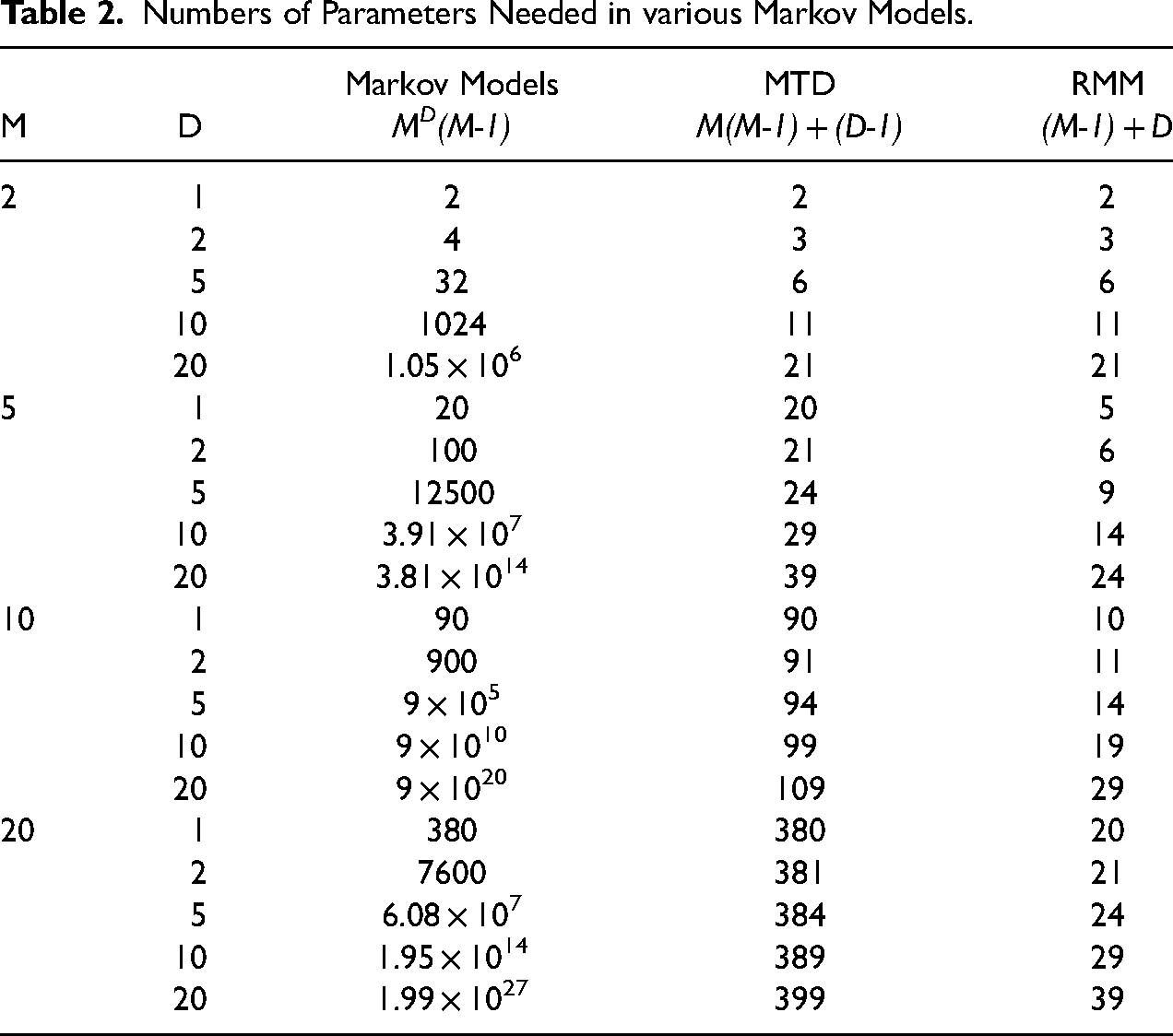
Markov models offer a simple and easily interpretable model of sequential dynamics. In Markov models, the generative process behind a sequence is modeled as a probability of an element conditioned on the preceding D elements. Markov models represent probabilities of elements in a sequence as a conditional distribution over a specified number of preceding elements. A Markov model of order D will provide a distinct conditional probability for every element given every possible subsequence of length D. The number of parameters required for a one-step Markov model scales with $N^{2}$ , where N is the number of possible states. A two-step Markov model scales with $N^{3}$ and so on for higher-order models. For any nontrivial amount of dependence, the number of parameters quickly becomes impractical.

Many simplifications to the standard Markov model have been proposed to reduce the number of parameters, including those of Jacobs and Lewis (1978), Pegram (1980), and Logan (1981). However, the current standard for parsimonious Markov modeling is Raftery’s (1985) mixture transition distribution model (see also Raftery and Tavare 1994; Berchtold and Raftery 2002; Islam and Chowdhury 2006). Mixture transition distribution (MTD) models significantly reduce the number of parameters necessary by assuming each transition is a linear combination of transitions between conditioning states. This approach greatly increases the ability to create higher-order Markov models, requiring only one parameter per step. Though better than other Markov models, MTD models still scale with the square of the number of possible states in a sequence, making the models less practical as the number of states increases.

Autoregressive Models

An alternative approach to modeling recurrent processes can be found in the vast literature on autoregressive models. In the simplest sense, an autoregressive model is a model that uses an outcome variable to predict future outcomes, typically continuous variables. Whereas Markov models tend to allow complex patterns of dependencies, autoregressive predictions are produced from observed sequences by modeling dependencies with specific coefficients. Thus, autoregressive models often take the form of a linear combination of previous observations. In this way, autoregressive models capture many periodic features of the data, limited only by the number of lags, or past observations, the model incorporates.

The use of lagged outcomes as a predictor of current outcomes is gaining popularity in sociology, particularly within economic sociology (e.g. Goldstein 2018; Castilla 2011) and spatial analysis (e.g. Ody-Brasier and Fernandez-Mateo 2017). However, autoregressions are most commonly found within the social sciences in econometrics under the ARIMA framework, where they are used to predict economic indicators while adjusting for cyclical effects, seasonality, and exogenous shocks. Standard AR models require a stationary process, i.e. a sequence where the distribution of variables remains constant across time, though ARMA models can account for changes in the average level of the dependent variable by incorporating a moving average (MA). A further variation to this framework models the process as the cumulation of observed differences between periods, i.e. integrated (I).

It should be noted that the ARIMA framework is explicitly not a generative model of time series. Few applications of ARIMA models are premised on the idea that measures generate themselves. Rather, ARIMA models focus on the effects of shocks. In this sense, these models represent the response of a system to an exogenous impulse. Like modeling a bell ringing after being struck (Box et al. 2011), the focus is on what happens (the toll of the bell) and how to represent it, rather than why it happened (what struck the bell).

Recurrent Event History Models

A related set of models can be found in event history analysis (Allison 1984). The standard Cox proportional hazard model can be extended to include possibilities of recurring events per individual by making assumptions about how subsequent events depend on prior events. For a more thorough review of these models, see Ezell et al. (2003) or Ozga et al. (2018).

The simplest extension of event history analysis to recurrent events can be found in the Anderson-Gill model (1982). The AG model assumes that the recurrence of an event is dependent only on the time since the last event, but not prior events. This assumption is somewhat analogous to a one-step Markov assumption in that only the last event or step affects the current time.

Prentice, Williams, and Peterson (1981) proposed two models that extend dependence beyond the most recent event by distinguishing between each subsequent recurrence of events. The first model estimates time between events, while the second models the event counting process. By incorporating event specific baseline hazards, the PWP models effectively treat the k^th recurrence as distinct from all other recurrences of the same event. This assumption deviates from a Markov assumption in that the whole history of events is relevant, causing the number of parameters to increase with both the length of the sequence and the number of different transitions.

Finally, Wei, Lin, and Weissfeld (1989) proposed a model of recurrent events that models total time until the k^th event happens, but includes only those individuals in the population who have not yet experienced the k^th event. Like the PWP models, the WLW model also assumes the k^th recurrent event is different from the k-1^th event, However, unlike the PWP model, WLW models treat everyone who has not yet experienced the kth event as at risk, even if they have not yet experienced the requisite preceding events.

While these three models account for the dependence of new events upon previous events, they do not model how recurrent events may be competitive with one another. For example, they do not allow events to be mutually exclusive at a given time, as is expected with typical sequential data. Steele et al. (2004) propose a discrete-time event history model with multiple competitive states like the model proposed below. However, unlike the event history models above, the Steele et al. model only allows for repeated events and does not model how events may be dependent upon previous states.

A Recurrent Multinomial Model

In this section, I introduce a multinomial regression model that accounts for tendencies of states to reoccur at various intervals. These sequential effects are accomplished by incorporating what I call a Markovian recurrence assumption. The resulting model thus draws directly on both Markov models and multinomial models, but also has features similar to recurrent event history models. Below, I first review the relationship between Markovian recurrence and Markov models. Next, I show how this assumption can be implemented in a simple multinomial framework. Finally, I introduce a general description of the model that incorporates covariates and discuss model specification and estimation.

For readers uninterested in the mathematical details, the subsection sections can be summarized as follows. By assuming that the probability of an element in a sequence is only affected by preceding elements with the same state, we can reduce the number of parameters needed to define an arbitrarily large Markov model. This parameterization can be described as an ordinary multinomial model with two sets of coefficients and covariates, one that describes recurrence patterns across the sequence and one that describes the baseline probability of each element. These two sets of parameters may interfere with one another, so care must be taken to ensure the model can be reliably estimated.

Markov Models and Markovian Recurrence

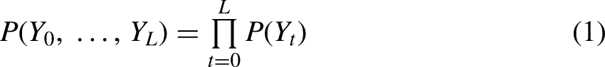
Suppose we have a sequence $Y = {Y_{0}, \dots, Y_{L}}$ of length L where the element $Y_{t}$ is a categorical outcome a from M possible states. For clarity, I will use the terms element to refer to an observed step in a sequence and states to refer to the possible values that observation can take. Sequences are composed of multiple elements, each of which may be drawn from the set of states.

All models of sequences reduce the overall complexity of the possible space of such sequences by adopting assumptions to force sequences into some compressed representation. The strictest model eliminates sequencing entirely, assuming that each element in the sequence is independent of every other. This representation can be modeled using a simple multinomial regression. Each sequence then has a probability defined by the product of the probabilities of its elements:

\begin{matrix} P (Y_{0}, \dots, Y_{L}) = \prod_{t = 0}^{L} P (Y_{t}) \end{matrix}

(1)

Markov models provide a more realistic representation by incorporating dependence between successive elements. The well-known Markov assumption assumes that elements in a sequence are conditionally independent given the D elements immediately preceding them. A Markov assumption of order D represents the sequence as:

\begin{matrix} P (Y_{0}, \dots, Y_{L}) = \prod_{t = 0}^{L} P (Y_{t} | Y_{t - 1}, \dots, Y_{t - D}) \end{matrix}

(2)

Using the notation from Berchtold and Raftery (2002), a first-order (D = 1) Markov model can then be written as:

\begin{matrix} P (Y_{0}, \dots, Y_{L}) = \prod_{t = 0}^{L} P (Y_{t} = a_{0} | Y_{t - 1} = a_{1}) = q_{a_{1} a_{0}} (t) \end{matrix}

(3)

where

q_{a_{1} a_{0}} (t)

is a potentially time-varying probability of transitioning from a₁ to a₀. A matrix

Q = [q_{a_{1} a_{0}}]

formed from these transition probabilities would have M² elements and M(M-1) degrees of freedom. For higher-order (D > 1) models, the transition matrix

Q = [q_{a_{D} \dots a_{1} a_{0}}]

grows to have dimension M^D x M with M^D(M-1) degrees of freedom (Table 1).

Table 1.

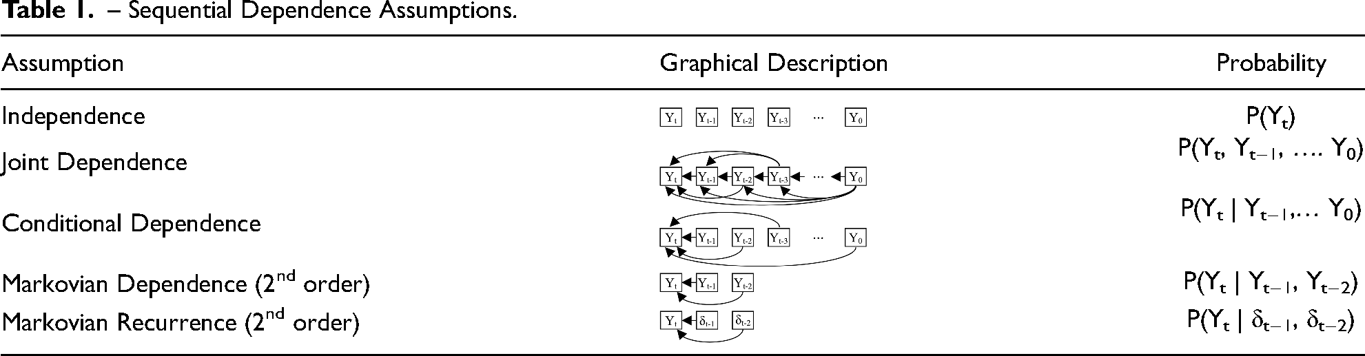
– Sequential Dependence Assumptions.

Assumption	Graphical Description	Probability
Independence		P(Y_t)
Joint Dependence		P(Y_t, Y_t−1, …. Y₀)
Conditional Dependence		P(Y_t \| Y_t−1,… Y₀)
Markovian Dependence (2^nd order)		P(Y_t \| Y_t−1, Y_t−2)
Markovian Recurrence (2^nd order)		P(Y_t \| δ_t−1, δ_t−2)

MTD models remove this exponential growth in parameters by assuming that the effects of successive lagged elements can be represented as a linear combination of a single lag transition matrix: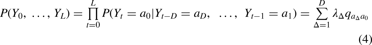

\begin{matrix} P (Y_{0}, \dots, Y_{L}) = \prod_{t = 0}^{L} P (Y_{t} = a_{0} | Y_{t - D} = a_{D}, \dots, Y_{t - 1} = a_{1}) = \sum_{Δ = 1}^{D} λ_{Δ} q_{a_{Δ} a_{0}} \end{matrix}

(4)

The Q matrix remains the same size as the first-order Markov model transition matrix, while each successive lag included in the model only requires a single extra parameter

λ

. This allows MTD models to represent sequences with only M(M-1) parameters for the transition and D parameters for the lagged effects. This parameterization eliminates the exponential growth from lagged effects, but retains quadratic growth in parameters from the number of states. While this is a far more parsimonious representation, the number of parameters needed may still become unworkably large for even a moderate number of states (as shown in Table 2).

Table 2.

Numbers of Parameters Needed in various Markov Models.

M	D	Markov Models	MTD	RMM
M	D	M^D(M-1)	M(M-1) + (D-1)	(M-1) + D
2	1	2	2	2
	2	4	3	3
	5	32	6	6
	10	1024	11	11
	20	1.05 × 10⁶	21	21
5	1	20	20	5
	2	100	21	6
	5	12500	24	9
	10	3.91 × 10⁷	29	14
	20	3.81 × 10¹⁴	39	24
10	1	90	90	10
	2	900	91	11
	5	9 × 10⁵	94	14
	10	9 × 10¹⁰	99	19
	20	9 × 10²⁰	109	29
20	1	380	380	20
	2	7600	381	21
	5	6.08 × 10⁷	384	24
	10	1.95 × 10¹⁴	389	29
	20	1.99 × 10²⁷	399	39

To address this issue, I adopt a modified version of the Markov assumption that focuses only on whether the current element is recurrent from the previous D elements and not on what the previous D elements were. I define this Markovian recurrence assumption as assuming that elements in a sequence are conditionally independent given whether the D elements immediately preceding them are the same as the current element. Informally, this assumption allows the probability to be proportional to some function of recurrences, rather than states:

\begin{matrix} P (Y_{t} | Y_{t - 1}, \dots, Y_{0}) \propto f (Y_{t}, δ_{t - 1}, \dots, δ_{t - D}) \end{matrix}

(5)

where

δ_{s}

is shorthand for Kronecker delta function

δ_{Y_{t} Y_{s}} = δ (Y_{t} = Y_{S})

which is 1 if

Y_{t} = Y_{s}

and 0 otherwise. The precise description of the function f will be stated in more detail in the next section.

Rather than modeling all transitions from past observations to new observations, this models only how observations reoccur based on past observations. When modeling the probability of an element being in state A, the states of preceding elements only matter to the extent that they are the same, i.e. A or not A. This assumption contrasts with the standard Markov assumption where the specific state of an element (A, B, C, D, etc.) provides unique information about the probability of A.

The Markovian recurrence assumption has two important implications. First, all states are treated nominally. The reoccurrence of one state is the same as the reoccurrence of other states, other things being equal. Second, the appearance of an element of a given state is primarily influenced only by past elements with the same state. No preceding states may make A more or less likely to occur, apart from A itself. Transitions from B to A are the same as C to A. Obviously, if either of these is not a good description of the phenomenon of interest, the model would be expected to fit poorly. The first implication may be slightly weakened with appropriate covariates, as I will discuss in the empirical example below. However, if the specificity of transitions states is important, i.e. the second implication is not an accurate description, then it is likely that an MTD model would be a more effective and appropriate modeling choice.

To be clear, Markovian recurrence does not require less information than standard Markov assumptions. Like the standard Markov assumption, a Markovian recurrence assumption requires full information about past samples. The probability of each element is a function of its own previous occurrences. Of course, to ensure that the predictions are a probability distribution and sum to one, all past samples are needed to compute the proper normalizing constant (i.e. denominator).

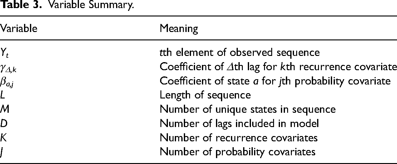
The benefit of this assumption, then, is not a reduction in information needed, but a reduction in the number of parameters needed to represent the distribution. Like MTDs, Markovian recurrence only requires one parameter per lag. However, since it only accounts for whether elements are the same or not, the Markovian recurrence assumption also only requires one parameter per unique element to account for baseline probabilities. This means that a D step model requires only (M-1) + D parameters. Further statistical details may be found in the appendices. Appendix A describes limiting behavior and bivariate properties. Appendix B provides a Monte Carlo analysis of bias and computation time (Table 3).

Table 3.

Variable Summary.

Variable	Meaning
Y_t	tth element of observed sequence
γ_Δ,k	Coefficient of Δth lag for kth recurrence covariate
β_a,j	Coefficient of state a for jth probability covariate
L	Length of sequence
M	Number of unique states in sequence
D	Number of lags included in model
K	Number of recurrence covariates
J	Number of probability covariates

There are numerous parallels to be drawn between the present model and recurrent event history models. Both model the probability of a given state reappearing and both assume this probability is dependent upon prior states. However, there important differences in how these assumptions are incorporated in each model. The primary difference separating the present model from a repeated event history model is the emphasis on ordering rather than duration. Event history models, including discrete-time models, emphasize the time at which a new state will appear or when a transition between states will occur. Markov models (including the present model) by contrast assume that some transition will occur at each time step, even if the transition maintains the same state. Event history models are more interested in the average time until another event occurs and must account for censoring in the observational process. In contrast, discrete-time Markov models including the present model record observations either irrespective of time, i.e. sequentially, or at specified time points, thus focusing less on the time between events.

Whereas event history methods can easily estimate hazards of occurrence at any arbitrary time, Markov models explicitly ignore effects beyond a certain time window (as stated explicitly in the Markov assumption). On the other hand, event history methods also tend to assume a monotonically increasing hazard function, which makes representing more complex (i.e. non-monotonic) recurrence patterns difficult as it precludes the possibility of suppressing effects. The more limited time window of sequential methods allows time-varying promoting and suppressing effects to be modeled easily, albeit over a limited range. The limited range of sequential methods also allows them to model longer sequences with greater numbers of recurrences with greater efficiency than either the PWP or WLW models. In this respect, the current model is similar to the Anderson Gill model in that recurrent events are treated equally and are not viewed as qualitatively different events.

Multinomial Models with Recurrence

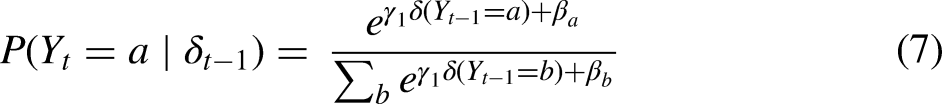
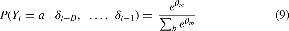
Equation 5 above does not fully define the functional form f of the probability distribution. While there are other ways of defining f, one obvious way to specify it is as a multinomial logistic function, which will produce a generalization of multinomial regression. This solution is attractive as the form and properties of multinomial regression are well studied and it allows researchers to draw on their existing intuition. To demonstrate this connection, I will begin by assuming a zero-order model, i.e. no recurrence based on past elements in the sequence. Replacing f in equation 5 with the multinomial logistic function and setting D = 0 produces: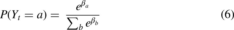

\begin{matrix} P (Y_{t} = a) = \frac{e^{β_{a}}}{\sum_{b} e^{β_{b}}} \end{matrix}

(6)

which is readily recognizable as the form of multinomial regression where

β_{a}

is the baseline coefficient for element a. As with all multinomial regressions, one state must be chosen as the reference category. For a first-order model (D = 1), we replace these coefficients with a linear combination of the baseline coefficient and the recurrence indicator:

\begin{matrix} P (Y_{t} = a | δ_{t - 1}) = \frac{e^{γ_{1} δ (Y_{t - 1} = a) + β_{a}}}{\sum_{b} e^{γ_{1} δ (Y_{t - 1} = b) + β_{b}}} \end{matrix}

(7)

where

γ_{1}

is the coefficient for the effect of recurrence after one time step and

δ

is defined as above. This form is interpretable as stating that the probability that element t takes on the state a is determined by its baseline frequency and whether it occurred at time t-1, normalized across all possible other states. As with the baseline coefficient

β

, the recurrence coefficient

γ

must be interpreted with respect to a reference. For a one-step recurrence (

γ_{1}

), the reference case is a state that did not occur one step before.

For higher-order recurrent models (D > 1), we can include further recurrence indicators and their coefficients by generalizing the exponent as the linear combination of all recurrence effects (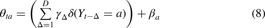 $γ_{1}, \dots, γ_{D}$ ) and the baseline coefficient $β$ :

\begin{matrix} θ_{t a} = (\sum_{Δ = 1}^{D} γ_{Δ} δ (Y_{t - Δ} = a)) + β_{a} \end{matrix}

(8)

The probability of a then becomes:

\begin{matrix} P (Y_{t} = a | δ_{t - D}, \dots, δ_{t - 1}) = \frac{e^{θ_{t a}}}{\sum_{b} e^{θ_{t b}}} \end{matrix}

(9)

General Recurrent Multinomial Models

As with multinomial models, the linear function $θ$ in equations 8 and 9 can be generalized further to include covariates on both the state baseline and the recurrence. This produces a model that can account for systematic variations in the recurrence structure, comparisons between different sequences, and other external determinants of recurrence. The probabilities of each element are then proportional to a log-linear function of K recurrence covariates (z) and J element covariates (x). Recurrence coefficients γ will be estimated for each covariate k and each lag Δ. Element coefficients β will be estimated for each covariate j and each element a. Including these covariates produces the following score function:

\begin{matrix} θ_{t a} = \sum_{Δ, k}^{γ} z_{t - Δ, k, a} δ_{t - Δ} + \sum_{a, j}^{β} x_{t - Δ, j, a} \end{matrix}

(10)

where Z is an LxKxM array of recurrence covariates, X is an LxJxM array of covariates for each step in the sequence for each element, and the subscript t is used to denote the position in the sequence. γ and β are assumed to be DxK and MxJ matrices, respectively, of normally distributed variables with zero mean and a finite variance.

Skipping steps in the derivation, the log likelihood for this general model can be written as: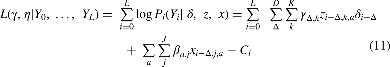

\begin{aligned} \begin{matrix} L (γ, η | Y_{0}, \dots, Y_{L}) \\ = \sum_{i = 0}^{L} \log P_{i} (Y_{i} | δ, z, x) = \sum_{i = 0}^{L} \sum_{Δ}^{D} \sum_{k}^{K} γ_{Δ, k} z_{i - Δ, k, a} δ_{i - Δ} \\ + \sum_{a} \sum_{j}^{J} β_{a, j} x_{i - Δ, j, a} - C_{i} \end{matrix} \end{aligned}

(11)

where C_i is the normalization constant. The first term in each represents the increase in the probability of an element being the same as a lagged element (relative to someone who did not speak Δ steps prior). Each γ parameter represents an additive component of the log of that increase, ignoring nonlinearities introduced by rescaling. Z can be used to represent influences of the recurrence structure of the sequence, including time, sequence setting, or other controls. The second term is directly interpretable as the baseline probability of an element appearing in the sequence. To keep the model identifiable, each probability covariate X will have one value defined as the baseline with its accompanying β fixed to zero. The coefficient β then represents the change in log odds relative to this baseline element. X can be used to incorporate influences on the state's probability, including presence or absence in a sequence, or relationship to other states.

Overall, the model functions much like a standard multinomial regression. As shown above, when there is no recurrence (D = 0), it becomes identical to a multinomial regression. When recurrence is included (D > 0), the multinomial probability for an element changes when that element has occurred in the last D observations. The nature of this change will vary depending on the recurrence coefficients γ and the covariates Z.

Defining the effect in this way does not require that the probability of an element has a stationary distribution or that recurrence patterns remain constant over the course of the sequence. Providing time-varying recurrence coefficients, such as position in the sequence, will allow recurrence to vary over the course of the sequence. For example, this could distinguish between (1) a question and answer pattern with multiple back and forths between two people and (2) a more open discussion among a large group of speakers and longer patterns of recurrence. In the same way, proper use of the probability covariates X allows for simultaneous modeling of multiple sequences, assuming they are generated by the same processes of recurrence. For example, sequences with different sets of states can be modeled collectively by providing a covariate specifying whether a given state is present in each sequence.

Model Specification and Identification

This full model as defined above can be specified with a given set of observed sequences Y, the degree of the model D, state covariates X, and, recurrence covariates Z. Modeling nonstationarity requires that X must include values for all possible states, as counterfactual probabilities cannot be inferred from other positions in the sequence. It is also important to note that models need not be saturated up to the maximum lag D. There is no need to include all lags lower than a desired lag. Constraining recurrence coefficients to be equal to 0 will have no effect on the estimated distribution. Additionally, because recurrence coefficients are not explicitly dependent upon preceding lags, terms for shorter lags may be omitted without conflicting with the coefficients of higher lags. This can allow estimation of long-range recurrence without creating a highly overfit model and may be particularly useful in modeling slowly changing sequences. It is also possible to define coefficients in reference to a different “clock”, e.g. time or proportion completed, or as a range of lags considered together.

Problems with identification may arise as a result of the competing effects of the γ and β coefficients. First, since a state's appearance in the sequence is likely to engender further appearances in the sequence, it is difficult to separate the influences of a state's baseline probability of appearing from the recurrence effects of having appeared. A very talkative person may not participate much at all in a discussion if they are never given the chance to speak. Conversely, a rather taciturn person may speak a lot if others continue to ask follow-up questions. While the differences between these two scenarios may become clear with sufficient observations, there will remain some analytic uncertainty with any limited amount of data.

As a result, the likelihood surface has multiple local maxima which could cause maximum likelihood estimation to produce unstable or suboptimal parameters estimates. To resolve this identification issue, I add the further assumption that the probabilities of elements do not differ greatly from the naïve, i.e. observational, probabilities and the reoccurrence effects are relatively small. This assumption is incorporated into the model using L₂ regularization (more commonly known as ridge regression) on the $η$ and γ coefficients, respectively:

\begin{matrix} \begin{matrix} L_{r} = L_{r} - λ_{1} ‖ γ ‖_{2} - λ_{2} ‖ β ‖_{2} \end{matrix} \end{matrix}

(12)

where

x_{2}

is the L₂ norm, i.e. the square root of the sum of squared values. Since coefficients are expected to have a mean of zero and are evaluated relative to a baseline of zero, the L₂ norm is effective at limiting the deviations from a uniform distribution.

Estimation & Inference

The parameters shown below were estimated using standard maximum likelihood estimation. All estimates were fit using the BFGS-L nonlinear optimization algorithm with an explicit gradient function. Standard error estimates were determined using computational estimates of the Hessian matrix.

Inferences about parameters and models are also similar to classic regression models. Since parameters are assumed to have a normal distribution, inferences about parameter estimates can be performed using conventional t-tests. Models can be selected using standard model selection metrics, i.e. AIC, BIC. Models can be tested against each other and against a null using likelihood ratio tests. Since parameters are normally distributed, Wilk's theorem says that the likelihood ratio will be expected to converge to a $χ^{2}$ distribution in the limit. This $χ^{2}$ distribution will have $‖ β ‖_{1} + ‖ γ ‖_{1}$ degrees of freedom.

Standard null hypotheses correspond to intuitive values. As mentioned above, when recurrence coefficients are equal to zero, they produce a conditional coefficient of 1, representing no effect on the distribution. Probability coefficients are measured relative to a fixed value of zero for the baseline element. With respect to null models of the whole sequence, a natural null model is a degree 0 model, which assumes no interdependence between elements in the sequence. However, when covariates are present, a better null model is a permutation test that reshuffles the order of the sequence while keeping the element frequencies constant. This allows the null to account for possible spurious effects from covariates. For this reason, degree 0 models are only appropriate for testing the recurrence structure and not the probability estimates.

Model Fit via Training/Test Split

One of the features of this model that is both an advantage and a drawback is that recurrence parameters are effective and efficient. Each additional recurrence parameter can have a sizeable impact on the predictions of the model and may be sensitive to even small patterns present in the data. At the same time, due to the relatively large number of parameters need for baseline probabilities, an additional recurrence parameter does not have a large effect on the overall number of parameters. This means that there is a danger of overfitting the model even when using model selection techniques designed to account for the number of parameters, e.g. AIC and BIC. For this reason, it is good practice to evaluate models in terms of their fit to data not used in the estimation process, i.e. a test set. Segregating available data into a training set, used to estimate parameters, and a test set, used to evaluate model fit, ensures that parameter estimates do not reflect the idiosyncratic noise found in the training set and that measures of model fit do not tend towards overfitting. This technique, which is standard practice in machine learning and other fields that frequently use models with a large number of parameters, is simply an alternative to AIC/BIC for balancing the bias-variance tradeoff.

Conversational Turn-Taking

This model is primarily motivated by the problems around analyzing conversational turn-taking (Gibson 2008). Though defined differently in various literatures, turn-taking in conversations is typically understood as the processes by which individuals negotiate successive participation in a conversation and the sequential patterns of speakers that emerge from these processes. Because turn-taking is involved in any social exchange, the conversational turn is often seen as a fundamental unit of social interaction and a component of the interaction order (Wilson et al. 1984; Sacks et al. 1974).

There is considerable disagreement across different research traditions about which features of turn-taking are relevant to social processes and theoretically interesting. Drawing from roots in ethnomethodology (Garfinkel 1984; Atkinson et al. 1984), the conversation-analytic (CA) tradition sees turn-taking as a process of meaningful action resulting in a roughly linear stream of conversation (Sacks et al. 1974; Schegloff 2007). Turns are intentional actions taken by an individual and, as such, must be understood within the full context of the interaction, the sequence of the conversation, and the flow of specific words from the perspective of the subjects involved. Thus for CA, understanding a conversational sequence requires delving into the moment by moment specifics of spoken interaction, including word choice, pronunciation, body posture, and attention of individuals, as well as the timing, cadence, and signaling found utterances between successive speakers.

As a consequence, analyses are restricted to very short, but rich, segments of video and transcripts. This has led CA scholars to study the process of changing from one speaker to the next in detail (Wilson et al. 1984; Duncan and Fiske 1977). Schegloff (2007) sees turn-taking sequences as fundamentally built by these short one-step adjacency-pairs. Conversational complexity progressively arises through speakers’ choices among types of adjacency-pairs, expansions on pairs, sequences of pairs, and sequences of sequences. However, the restricted length of exchanges and CA’s own theoretical orientation precludes such analyses from systematically investigating longer term recurrence, burstiness, or transient patterns in conversational participation.

Research building from the group processes literature (Bales 1950) and expectation states theory (Berger et al. 1972) sees turn-taking patterns as both a result of pre-existing expectations about participants and a process by which new expectations are constructed. The focus on a group member's preconceptions about the traits of other group members has led to an interest in the effects of status, gender, and authority on the resulting speech. While these effects include simple turns, most research focuses on occurrences of interruptions (Cannon et al. 2019; Gibson 2005a; Smith-Lovin and Brody 1989), laughter (Robinson and Smith-Lovin 2001), topic changes (Gibson 2010; Okamoto and Smith-Lovin 2001), supportive speech (Johnson et al. 1998), and directions (Johnson 1994).

Early studies focused on how such conversational features were related to the characteristics of the participants, though later research has shown that such a priori expectations about other participants are often less important than the dynamics of the conversation itself. Sequencing effects and other processes endogenous to the conversation itself are better predictors of conversational outcomes than are individual characteristics (Shelly 1997; Cannon et al. 2019; Okamoto and Smith-Lovin 2001; Fişek et al. 1991; Smith-Lovin and Robinson 1992).

Gibson's (2003; 2005b) work on turn-taking shows a fruitful intermingling of both CA and expectation-states traditions. Gibson (2003) proposed analyzing the processes within conversation using both the sequence of speakers and the direction of the utterances. His participation shifts represent turn-taking with the combination of two speaker-receiver dyads: the speaker and intended target, followed by a subsequent speaker and intended target. This framework is able to encode more complex conversational dynamics, including turn receiving, claiming, and usurping. Using this more complex representation further enabled systematic investigation of the relationship between sequencing and individual characteristics and status (Gibson 2005b).

Gibson's dyadic and triadic formulation of turn-taking made it a natural fit for formalization into a network based statistical model, known as relational event models or REMs (Butts 2008). Building from an event history framework, REMs can elegantly capture the timing of dyadic (speaker-receiver) events. However, due to the high dimensionality of the network modeling space, parameter estimation is generally limited to two successive events. Even simple turn-reclaiming requires sequences involving three speakers (i.e. three-paths in network terminology) which can be difficult to estimate reliably.

More conventional statistical modeling approaches to turn-taking, like those discussed in previous sections, also suffer from some significant problems (Gibson 2008). In many though not all respects, recurrent multinomial models offer advantages over other models. First, successive speaking turns are unlikely to have stable ordering patterns (Sacks et al. 1974) that could be suitably described by a static bivariate distribution, as done with Markov modeling (Cappella 1980). While there may be a strongly defined interactional order, interactional orders do not amount to dictating who speaks when. In any multi-person conversation, turn ordering is not only determined by the stage and topic of the conversation and speakers’ predispositions towards participation, but is also directly controlled by individual speakers selecting subsequent speakers (Wilson et al. 1984) and by listener's actions to inject themselves into the conversation. Participation shifts are often achieved by directly indicating who should speak next, perhaps by addressing them by name or asking them a question (Gibson 2003, 2005b). In contrast, it is also possible, though rude, to designate a non-speaker, as in instructing someone to be quiet. Both of these features are transient effects and would not be well described by a stationary Markov transition matrix.

Second, speaker participation in conversations tends to occur in bursts. Speakers may claim and reclaim multiple turns before stepping back to listen and let others contribute. In this way, turn-taking occurs on different levels: small turns, i.e. speaker by speaker, and big turns, i.e. alternating periods of participation and observation. Analytically, burstiness requires looking for recurrence on multiple scales, a short scale and a longer scale.

Additionally, turns in a conversation, while meaningful, are also cheap. A single two-party exchange may be complicated by elaborations (Jefferson 1988; Schegloff 2007), clarifications and conversational repair (Schegloff 1992), and role enforcement and interactional repair (Goffman 1959). A conversation dominated by an exchange between two speakers may produce more complicated sequences of turns as others interject, question, and so forth. While not able to analytically distinguish such expansions, recurrent multinomial models can reveal the frequency of extensions through higher rates of lagged recurrence.

Lastly, though turn-taking may be a fundamental component of conversation, conversational dynamics are about more than just sequences of turns. The topic and context of the conversation will determine the conversational norms to be enacted and enforce and when the conversation will end (Sacks et al. 1974). The statuses, interests, and inclinations of the speakers will guide the topic of conversation, the relative rates of speaking, attention, and interruptions (Gibson 2003; Okamoto and Smith-Lovin 2001; Cannon et al. 2019). A workable model of turn-taking must at a minimum permit the use of additional covariates relating to the content of the speech.

Despite these advantageous features, recurrent multinomial models are not ideal for all investigations of conversational turn-taking. The assumption about discrete-time steps in the sequence generation obscures time-dependent conversational processes. Naturally, the hazard of interruption will increase the longer a speaker's turn lasts. Pauses in speech provide opportunities for other speakers to take the floor, though the current speaker may continue if there are no takers (Maynard 1980). As evident in the example below, transcription choices about when one speaker's turn ends and another begins or how to account for simultaneous speakers will inevitably affect the outcomes of the model.

CA researchers in particular will find fault with this representation. For example, Boden (1994) highlights the need for greater attention to sequencing in organizational interactional processes, but she explicitly decries the “mechanistic use of lagged variables in multivariate analysis, … event history, or sequential analysis” (Boden 1994: 208) as what Duncan (1984:226) called statisticism, namely the naïve identification of measurement and statistics with research. Certainly, recurrent multinomial models are incapable of a full dynamic or semantic representation of conversational sequencing. However, like virtually all quantitative methods, using an imperfect measure while recognizing its limitations and omissions does not necessarily imply a misrepresentation of the phenomenon of interest. I suggest that, although recurrent multinomial models are reductive and fall short of a full explanation of turn-taking processes, they provide better indicators of long sequential patterns in conversation than other modes of analysis precisely because they are able to compress the details of interaction into a simpler form.

Data & Example

FOMC Meetings

The following examples use data from transcripts of the Federal Open Market Committee (hereafter FOMC). The FOMC is one of the principal decision-making bodies at the Federal Reserve, tasked with determining interest rates and overseeing the growth of the money supply, primarily through the buying and selling of U.S. Treasury securities. The FOMC consists of twelve voting members: the seven members of the Federal Reserve Board of Governors, the President of the New York Federal Reserve Bank and four of the other eleven regional Federal Reserve Banks who serve on a rotating basis. Meetings also include a range of other Federal Reserve staff and economists, as well as some vice presidents of regional banks. In any given meeting, there are between 20 and 30 different people speaking at one point or another.

Meetings are led by the chairman of the Board of Governors and generally follow a standard format, beginning with reports on the general economic situation by staff economists. Regional bank presidents then weigh in with reports from their own district and some of their own economic analyses. The last third of the meeting is dedicated to an open discussion of the economic climate and future, oriented towards a decision about whether to raise, lower, or maintain current interest rates. Meetings typically last about a day and a half, including breaks (Figure 1).

Figure 1.

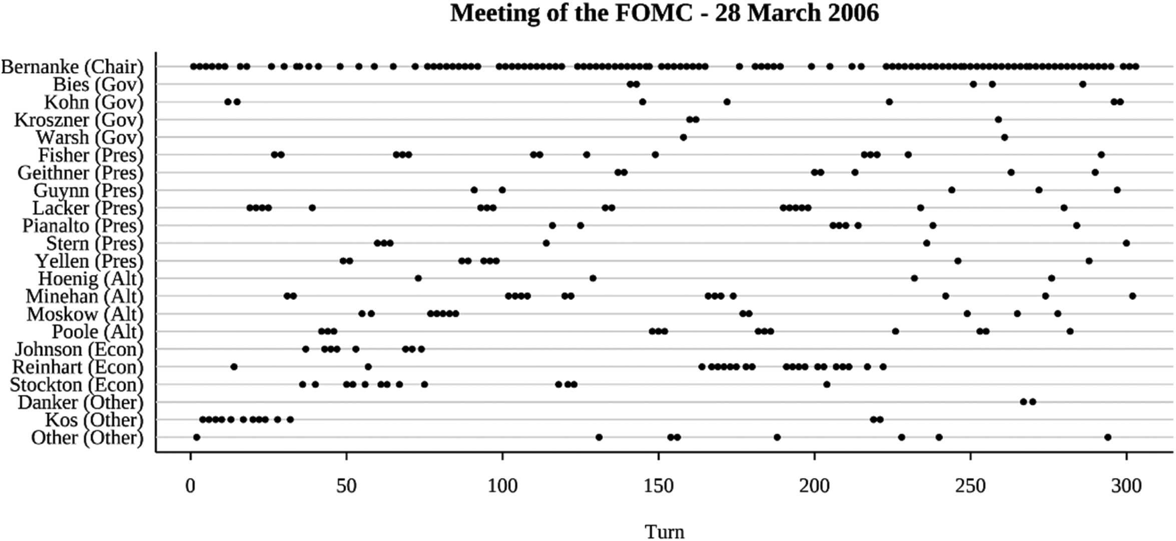
A typical meeting sequence.

The analysis below uses the transcripts from March 2006 through December of 2010, the beginning of Ben Bernanke's tenure as chairman through to the end of the 2008 financial crisis. There was a total of 39 FOMC meetings during this period. This set was randomly split into 20 meetings for training the model and 19 meetings for testing the model and validating the results. For each meeting, sequences were composed of the names of each speaker in order from start to finish. By the convention in the transcript, a new speaker is specified when the speaker changes or when there is a formal break in the meeting. The average meeting had 274.05 turns (sd = 82.00) with an average 202.91 words spoken per turn (sd = 414.95).

FOMC meetings are orderly and formal discussions. In his role as chairman (Boden 1994; Gibson 2012), Bernanke occupies a central position throughout most of the discussion, though not as central as some of his predecessors, and keeps the discussion close to the predefined agenda. As such, there are only short periods of wide-ranging discussion and few occurrences of backchanneling or side comments.

Still, transcripts represent “linearized” accounts of the actual meetings in at least two respects. First, transcriptions omit any simultaneous speakers, listing only one speaker at a time. The polite and orderly nature of the meetings suggests that such occurrences are relatively infrequent, but there is no way to be certain given the data available. Interruptions are noted in the transcript, indicated by a hyphen at the end of the utterance, but as audio recordings are not available, how frequent unmarked interruptions were remains unknown. Second, transcripts report all consecutive speech by the same speaker as a single turn, omitting any pauses or failed interruptions. This somewhat artificial feature will create a predictable suppressive effect on recurrence after one lag and a high level of alternation in speakers. Other conventions for coding turns, such as time or word count, would produce different patterns.

Measures

The basic speaker sequence and the covariates included in each model are defined as follows.

Speakers. The sequence of speakers was extracted from the official transcript of each meeting. The rare occurrence that multiple speakers are identified, as with laughter, are removed. Coffee breaks and other intermissions are also omitted. To increase the stability of the estimate and reduce computation time, speakers who spoke less than 10 times over the 20 training meetings were replaced with “Other”.

Sequence fraction completed. I measure changes in recurrence structure over the course of the meeting using the fraction of the meeting that has been completed. This is defined as the number of speakers up to this point divided by the total number of speakers in the meeting. It should be noted that this is a post hoc measure, since the total number of speakers is not available while the meeting is in progress. This is not a major issue for our purposes here because (a) there is no attempt to make a causal argument, and (b) by design and tradition, FOMC meetings are highly structured with roughly the same meeting duration and number of presentations, questions, and thus utterances in every phase of the meeting.

Role. The role of each speaker will be represented by their job title and position relative to the committee. This includes the FOMC chair (always Bernanke for this period), members of the board of governors, and voting regional bank presidents, and nonvoting alternate members (who were also presidents). I also include economists who, though not officially on the committee, are typically responsible for presentations of analyses and data at the beginning of the meeting. All other speakers were put into a separate category. This includes, but is not limited to, all speakers replaced with “Other”. “President” was the most frequent role and was used as a baseline.

Holding the floor. I measure short bursts in conversational participation, which I will call “holding the floor” (Cappella 1985), to capture the tendency of people who have spoken in multiple turns to continue to reclaim their turn. A speaker's holding of the floor value is defined as the proportion of turns the specific speaker has taken over the last 10 overall turns.

Word count. I also measure the length of each utterance as the number of separate words in the utterance. To account for the high rightward skew of this distribution, I use the logarithm of these values.

Analyses & Results

I begin with a basic analysis of the recurrence structure of the meetings. Table 4 shows the estimated recurrence coefficients for 8 different models with orders from 0 to 16. The zeroth-order model (model 1) includes no recurrence coefficients and serves as a baseline for evaluating whether recurrent models are an improvement over an unordered estimate. Still, it uses 455 parameters to estimate the relative probabilities of each speaker in each meeting. This amounts to about 22 different speaker coefficients per meeting, not including the reference speaker (Bernanke). Since these parameters are largely analogous to multinomial coefficients, I will omit further discussion.

Table 4.

Basic Recurrence Models.

	Dependent Variable: Speaker Sequence
	(1)	(2)	(3)	(4)	(5)	(6)	(7)	(8)
Lag
1		−0.995***(0.090)	−0.520***(0.103)	−1.835***(0.107)	−2.099***(0.110)	−2.246*(0.111)	−2.456***(0.114)	−2.606***(0.115)
2			3.464***(0.033)	2.897***(0.035)	2.669***(0.035)	2.571***(0.036)	2.481***(0.036)	2.423***(0.036)
3				2.284 ***(0.053)	1.719***(0.059)	1.593***(0.060)	1.503***(0.062)	1.454***(0.062)
4				1.569***(0.043)	1.169***(0.047)	1.018***(0.047)	0.915***(0.048)	0.882***(0.048)
5					1.213***(0.056)	0.855***(0.060)	0.731***(0.061)	0.694***(0.061)
6					1.137***(0.048)	0.785***(0.053)	0.579***(0.054)	0.523***(0.054)
7						0.875***(0.058)	0.463***(0.063)	0.400***(0.063)
8						0.981***(0.050)	0.623***(0.056)	0.540***(0.057)
9							0.373***(0.065)	0.254***(0.066)
10							0.524***(0.059)	0.364***(0.060)
11							0.842***(0.060)	0.490***(0.065)
12							0.716***(0.055)	0.452***(0.061)
13								0.278***(0.066)
14								0.464***(0.063)
15								0.751***(0.061)
16								0.502***(0.059)

Sequence Length	6102	6012	6102	6102	6102	6102	6102	6102
Parameters	455	456	457	459	461	463	467	471
Likelihood	−21869	−21812	−15915	−14772	−14374	−14141	−13878	−13723
AIC	44649	44536	32744	30463	29669	29209	28689	28387
BIC	47705	47599	35814	44546	32766	32318	31826	31551
Chi2	-	114***	11908***	14194***	14992***	15456***	15984***	16294***
Test Set Likelihood	−15447	−14861	−13486	−13097	−12978	−12984	−12942	−12907

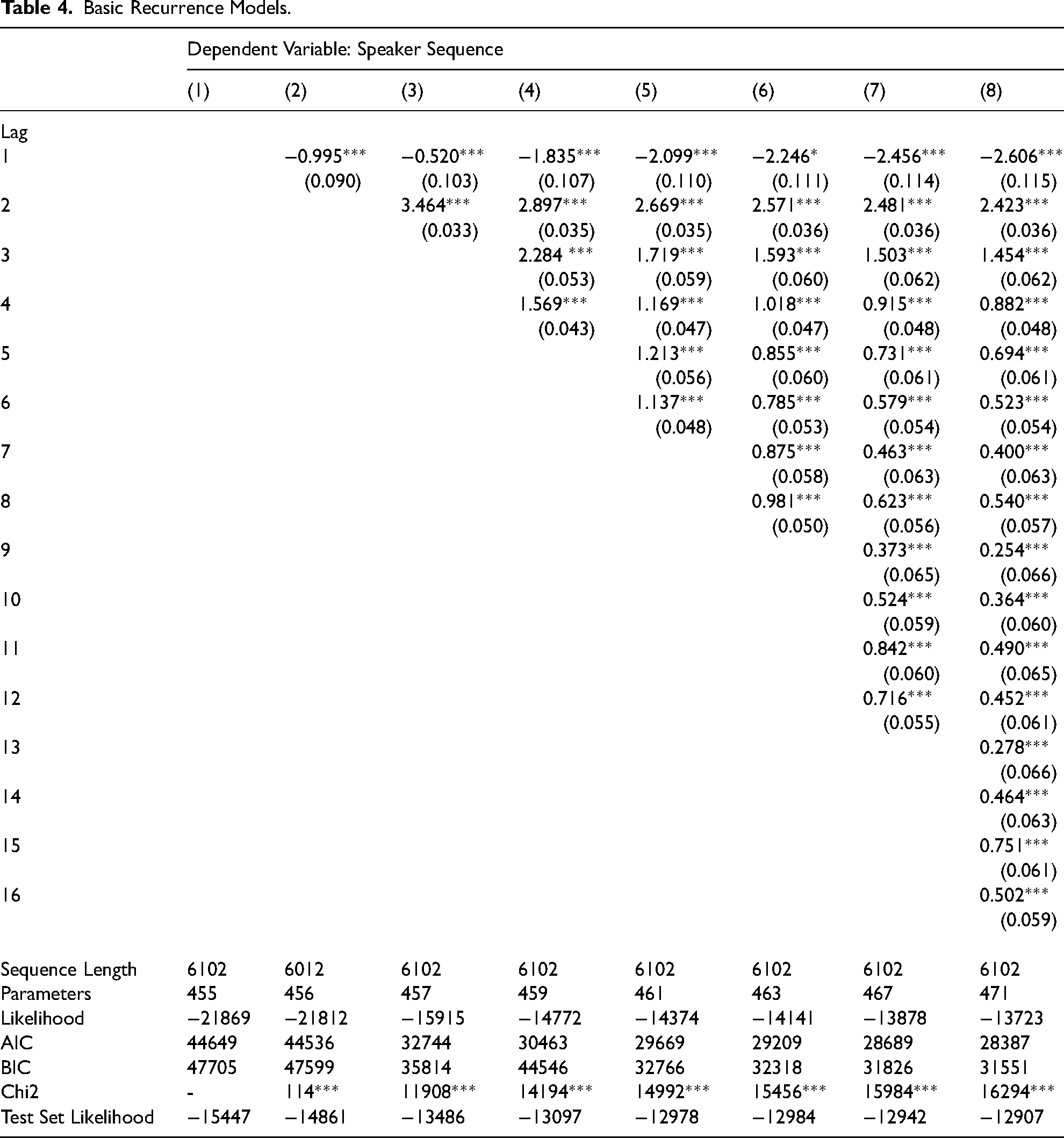
Model 2 with degree 1 shows an improvement over model 1 by all measures. The first lag coefficient is significant and negative, indicating that speakers are not likely to speak again immediately afterward. This basic turn-taking is to be expected in most conversation (Sacks et al. 1974). This effect was anticipated given the structure of the transcripts and can serve as a kind of validity check on the functioning of the model. Indeed, every model shown below has a large negative and highly significant effect for the first lag.

Models 3 through 8 show an increasing number of lags included and increasing model fit on all measures. As expected, parameter estimates across models do not vary to a large extent. Lag 2 is significant and positive in all models, meaning that turn reclaiming is highly likely. The addition of this lag in Model 3 corresponds to the biggest improvement between successive models. This is because turn reclaiming (lag 2), though less common than basic turn taking (lag 1), does much more to predict which element will come next in the sequence. Lag 1 says that the next speaker could be any speaker but the previous speaker, while lag 2 says that the next speaker will be a specific speaker, i.e. the one who spoke two turns ago.

Lags 3 through 16 are significant and positive as well and tend to be smaller than the preceding lags. Diminishing effects of this sort are to be expected in most recurrent or autocorrelational processes, as processes tend to be less dependent on their history as distance increases. Still, there are two patterns in these coefficients. First, the coefficients do not monotonically decrease in higher lags, nor do they become insignificant. Even 16 turns later a previous speaker is still more likely to speak again than someone who has not spoken in the last 16 turns. Such recurrence means there are longer term patterns of participation across discussions than can be captured in simple short exchanges. Second, there are slight indications of alternation in recurrence coefficients. Lag 7, 9, and 13 are noticeably (though not significantly) smaller than the preceding and successive lags. This could indicate a tendency to speak within a largely dyadic turn-taking structure, such as that between a primary speaker and questioners.

Patterns of coefficients were largely identical across models, though effect sizes decrease as additional lags are included. AIC, BIC, and test set likelihood continue to decrease with higher-order models, suggesting that patterns of recurrence up to 16 turns out are not overfitting the sequences. This reinforces the assertion made above, that recurrence parameters are “cheap” compared to the costs of accounting for multiple speakers.

Covariate Analysis

Models 1 through 8 accounted for recurrence patterns but did not investigate the determinants of those recurrences or how they varied across speakers or with time. Table 5 shows the results from models that include explanatory covariates. Based on the preceding set of results, I fit models of order 16. Note that parameter size increases more quickly across models than it did in table 4. Each covariate requires one parameter for each lag, thus adding 16 parameters for each additional covariate. Still, the total number of recurrence parameters is relatively small compared to the number of probability parameters (see model 1). By most measures, model fit across all models improves over the base order 16 model (model 9)², suggesting that these covariates are worth the increased complexity.

Table 5.

Results for Models with Recurrence Covariates.

		Recurrence Models
		(9)	(10)	(11)	(12)	(13)	(14)
	Number of Lags	16	16	16	16	16	16
Recurrence Covariates	Fraction Completed		X				X
	Role			X		X	X
	Holding the Floor				X	X	X
	Word Count				X	X	X

	Sequence Length	6102	6102	6102	6102	6102	6102
	Parameters	471	487	535	503	567	583
	Likelihood	−13895	−13538	−12978	−13666	−12712	−12703
	AIC	29732	28049	27027	28339	26557	26573
	BIC	31895	31320	30620	31717	30365	30489
	Chi2	-	715***	1833***	457***	2367***	2383***
	Test Set Likelihood	−12888	−12450	−12645	−13717	−14059	−13995

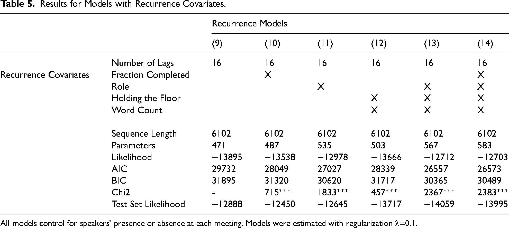
All models control for speakers' presence or absence at each meeting. Models were estimated with regularization λ=0.1.

The best fitting model varies across different measures of model fit. Model 13 has the lowest AIC and BIC, while the test set likelihood is best for models 10 and 11. Interestingly, the test set likelihood for models 12 through 14 is worse than that for even the base model (model 9). This is investigated in more detail below. For the sake of demonstration of the model's properties, I choose to display the results for model 13.

The selection of model 13 is also important for what it does not model. Specifically, the results of the model fit suggest that the time-varying parameter is not particularly important across the sequences. Put differently, the speaking norms in FOMC meetings are constant across the course of the meeting.

Figure 2 shows parameter estimates for model 13, split across types of covariates. As with model 8, the main effect of the recurrence parameters shows turn-taking (negative effect for lag 1) and turn-reclaiming (positive effect for lag 2), followed by diminishing effects. Unlike the simple models above, speakers are more likely to speak again for only up to 6 more turns, after which coefficients are largely insignificant. Lags 8 and 11 remain significant. Lag 8 may be a reflection of alternation patterns, while lag 11 seems to be an anomaly. Still, these results suggest that big participation turns last between 6 and 11 speakers.

Figure 2.

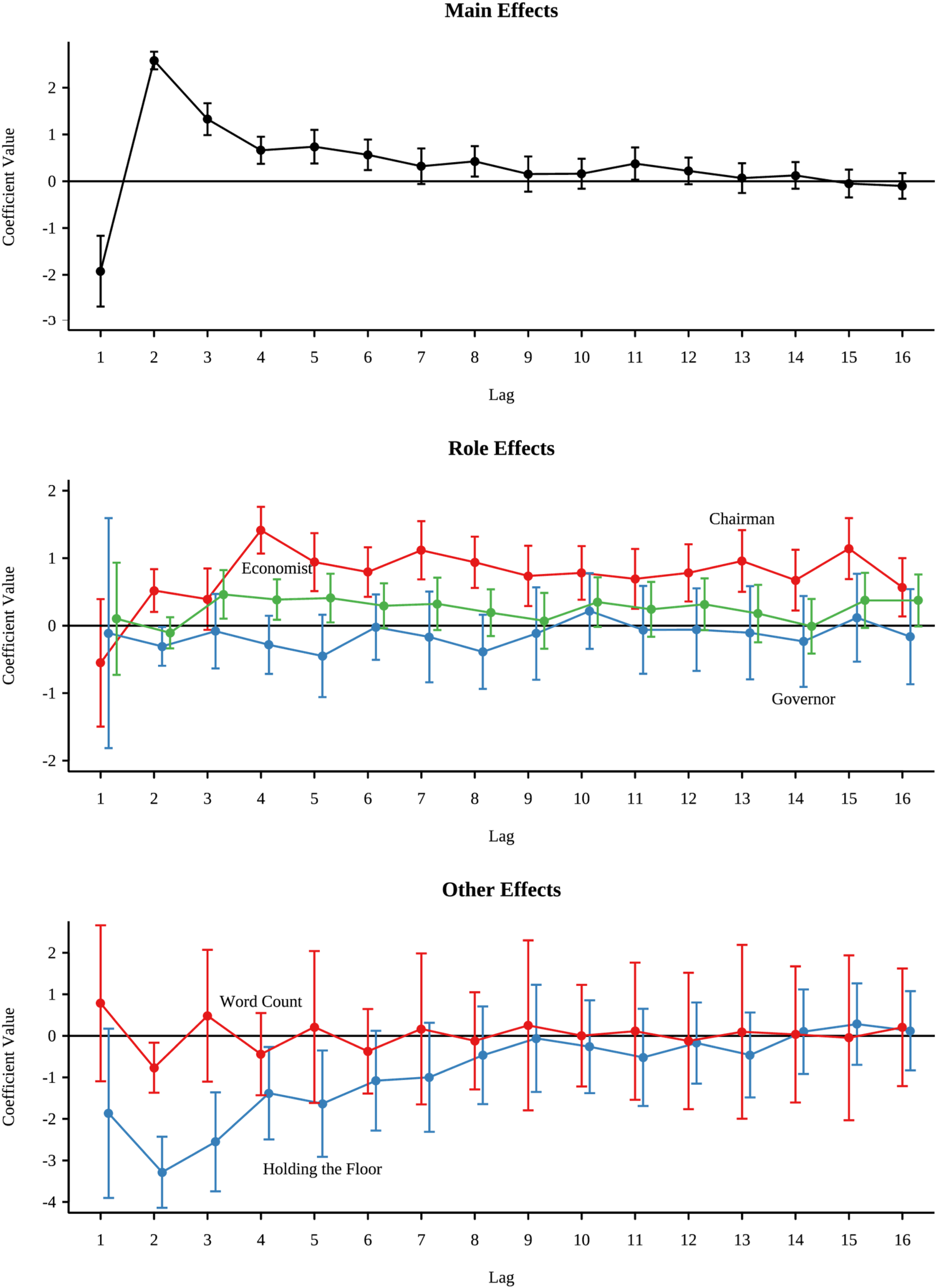
Estimated recurrence effects (model 13). Role effects are estimated relative to bank presidents. Alternate committee members had no significant differences from presidents and are omitted for clarity.

This pattern shows some variation across roles, though all roles respect the basic turn-taking (lag 1) norm. Relative to bank presidents (the baseline), the chairman is significantly more like to speaker again on all turns, except for lag 3. This is a further indication of alternation beyond simple turn-taking. This increased recurrence also helps to explain why the baseline lag parameters are not consistently significant beyond lag 6. The patterns of recurrence up to lag 16 that were shown in model 8 were due to Bernanke's disproportionate speaking. Regional governors are slightly less likely to reclaim their turn than were bank presidents.³ Economists are more likely to speak again on turns 3 through 5, reflecting their role in providing detailed reports and responding to questions and comments from the voting members of the FOMC.

As the bottom panel shows, there are other norms against members dominating the conversation (apart from the chairman). Taking a very long turn speaking (in terms of word count) means speakers will be less likely to reclaim their turn. Members will choose to give a long comment or multiple comments, but not both. However, after letting a person speak (lags 1 and 2), long-winded speakers do not differ from others. In contrast, having taken a number of turns in a short period (“holding the floor”) appears to suppress participation up to 5 turns. This pattern of holding the floor suggests that big turns in participation are separated by a period of abstention. This is consistent with the norms of the FOMC in allowing all committee members equal opportunity to participate, excluding the chairman.

Test Set Comparison

As with all complex models, there are many ways1 these models can fail that are not necessarily captured by standard model fit metrics. As discussed above, the large parameter space suggests that a test and training set methodology can be helpful to protect against overfitting. Overfit models would be a considerably better fit on the training set than they would on the test set. Figure 3 shows a comparison of the log-likelihood of the individual FOMC meetings, normalized by meeting length. There appear to be no major differences in model fit between the training and test sets.

Figure 3.

Comparison of results for training and test Set. Filled circles indicate meetings in the training set. Open circles indicate meetings in the test set.

Surprise

Surprise, an information theoretic measure, is useful for evaluating models at the level of individual turns. Surprise, also called self-information, is simply the negative log of probability, giving it a more convenient scale for evaluating how likely observations are. Observations with low surprise, corresponding to a high probability, are much more likely, while observations with a high surprise, and low probability, are less likely.

The surprise for the sequence of speakers in the first meeting in the dataset is shown in Figure 4. A degenerate model would have many observations with a very high surprise. This means that the model would deem the observed values as unlikely to appear in the sequence. What counts as a high surprise must be judged relative to the number and distribution of elements in the sequence. The expected surprise of each element if the sequence were distributed uniformly across the 22 unique speakers in the sequence is shown in Figure 4 using a horizontal dashed line.

Figure 4.

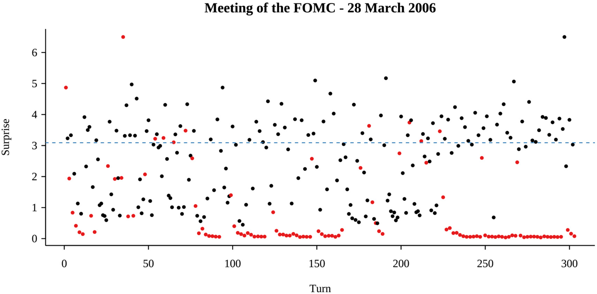
Surprise. Surprise ( $- \log \hat{p}$ ) for each element in a typical meeting. Red points indicate turns taken by Chairman Bernanke. The dashed line indicates expected surprise under a uniform distribution of speakers ( $- \log \frac{1}{S})$ .

Conversely, surprise can also be used to identify errors in the original data, rather than errors in the model. For example, in Figure 4, there are two points with a surprise greater than 6 and merit further inspection. The first is a case where Bernanke speaks twice in a row, which according to the transcription process should not normally be recorded as two separate turns. In this case, however, these turns were separated by a coffee break. The second case is an instance where an infrequent speaker (Pres. Guynn) interjects at a point when Bernanke is more likely to speak, as he had been taking every other turn for quite a while.

Robustness

The robustness of model estimates was tested by randomly introducing errors into the data, fitting a model to this corrupted data, and then evaluating the original data with the flawed model. Four methods for introducing error were tested: (1) inserting a random new element (e.g. ab→acb), (2) removing an existing element (e.g. abc→ac), (3) replacing an existing element with another (e.g. abc→adc), and (4) marking existing elements as missing (e.g. abc→a_c). For each method, erroneous data were constructed from the training data used above and changing a set percentage of the elements in the sequence. The percentage of errors was varied from 5% to 90%. This process was repeated 10 times for each method and level of error. The average and extreme values of the likelihood for each test are shown in Figure 5.

Figure 5.

Robustness analysis. The x-axis shows the percentage of data changed by one of the four processes. Solid lines indicate model likelihood on erroneous data. Dashed lines indicate likelihood of erroneous model on original data. Grey bars indicate the minimum and maximum likelihood out of 10 replications for each configuration.

Overall, models appear to be highly robust. The original data tends to fit the model better than the flawed data provided, suggesting that the models are able to identify recurrence patterns relatively accurately even when the data are imperfect. Models were able to maintain high likelihoods on the original data up to around 40% of data being errors, after which degradation increased more rapidly. As expected, removing elements or marking them missing caused markedly worse performance than inserting elements.

Discussion

This paper has presented a model of categorical sequences where the primary feature of interest is the recurrence of states. The Markovian recurrence assumption enables a parsimonious representation of autocorrelation-like properties across many states at the expense of the ability to explicitly model transitions from one state to another. The primary advantages of the recurrent multinomial model are two-fold: (1) the easily interpretable representation of lagged dependencies and (2) the ability to model sequences with a large number of states. The latter is achieved by reducing the number of parameters needed for each state in the sequence. This provides the capability to model longer sequences and long-term recurrences, where Markov and MTD models run into difficulty. An added benefit is that recurrent multinomial models allow nonstationary and covariate dependent processes can easily be modeled under the same framework.

These advantages are not without their limitations. Parsimony in parameters may not be desirable in all cases, especially when the Markovian recurrence assumption is unrealistic or counter to the research interests. When transitions between successive elements in a sequence are dependent upon the identity of the particular elements, this model will produce undesirable and highly biased results. In cases like this with sequential transitions, the Markov assumption is still more appropriate and MTD or similar models should be used.

A second significant limitation, particularly with respect to event history models, is the recurrent multinomial models are limited to conditions where only one event is possible at a time. This competition between states is built into the formulation of elements as a sequence and, to a lesser extent, the linear organization of orderly conversation. This property eliminates a great many phenomena from being analyzed with these models. It is possible that the Markovian recurrence assumption could be integrated into other models more suited for non-competitive categorical appearances, but this may simply recreate a discrete-time event history analysis.

A third limitation comes from combining naïve probabilities of state occurrence (β) with effects of recurrence (γ) to forming predictions. Monte Carlo simulations (Appendix B) reveal that this problem of identification results in a substantively small but consistently significant negative bias in recurrence parameters. Although this bias can be reduced by careful selection of the lambda parameters, it remains likely that recurrent multinomial models will produce poor model fit for highly unequal distributions of elements. This is was the case in the empirical example, where model fits improved significantly after accounting for Bernanke's disproportionate speaking role as chairman of the committee.

Model Extensions and Applications

The FOMC transcripts used above could be reanalyzed by redefining the sequence clock. Though speakers were modeled as discrete and timeless “turns”, the sequence could be defined in terms of word count, topic, or other similar features. A word count based sequence could, for example, split turns up every 100 words. This would provide a better view of recurrence as a temporal phenomenon and provided a better idea about how much time speakers are allotted. This would also likely reduce the apparent influence of Bernanke as chair since most of his utterances are short. This reanalysis could be achieved simply by preprocessing the data to split long utterances into shorter ones and reinterpreting what the coefficients implied.

While the multinomial framework requires each element in a sequence to have only a single value to ensure that predicted probabilities are modeled correctly, there is no similar constraint on the recurrence coefficients. This opens the possibility of modeling recurrence over ranges or groups of steps in a sequence, rather than just single steps. For example, one recurrence coefficient could be defined for lags 1–5 and another for lags 6–10, rather than needing 10 separate coefficients for lag 1 through 10. Conversely, there is no requirement that models be “saturated”, having a coefficient for every shorter lag.

Recurrent multinomial models may be used for direct and indirect research applications. The direct applications include modeling of empirical categorical sequences, similar to the example above. This could include many aspects of daily life where the recurrence of a state is not dependent upon specific other states, such as sequences of time use, occupational tasks, socializing habits, and travel patterns. Moving beyond the idea of recurrence as a temporal phenomenon, recurrent multinomial models may be useful for any kind of linearizable sequence of states or categories. For example, it would be possible to analyze the patterns of recurrence in texts, including the subject of sentence, dominant topic of a paragraph, style of argument, motif, or other identifiable and discrete feature.

Recurrent multinomial models could also be used indirectly for purely methodological purposes. As shown in the robustness analysis, recurrence patterns are stable in the presence of even a moderate number of errors. Additionally, the surprise diagnostic may enable identification of specific elements that are highly unlikely. Such analyses may be useful for data cleaning, such as identifying errors in sequence data or imputing the values of elements. Recurrent multinomial models could also help investigate the effects of state sequencing or timing on outcome distribution by generating a null model of counterfactual sequences with controlled generative processes.

Footnotes

Author's Note

A replication package including code and data used in the analyses is available on OSF at (DOI: 10.17605/OSF.IO/MEZ8J). An R package for running recurrent multinomial models is also available.

Associate Editor

Declaration of Conflicting Interests

The author(s) declared no potential conflicts of interest with respect to the research, authorship, and/or publication of this article.

ORCID iD

Michael Schultz

Notes

Author Biography

Michael Schultz is an assistant professor of Sociology at Indiana University Bloomington.

Appendix A: Statistical Properties

Appendix B: Simulation

Monte Carlo simulations were conducted to evaluate bias in parameter estimates and computational time. Three sets of simulations were conducted using parameters D, M, N, and L as described below. For each simulation, D true values of recurrence parameters were selected from a normal distribution with a mean of 0 and a standard deviation of 2. These values were chosen to provide a range similar to those of the empirical case. Baseline coefficients for each of the M states were set to 1.

Second, N observed sequences of length L were generated element by element according to equations 9 and 10. Third, models of order D were fit to these simulated sequences. These simulations only evaluate models with the correct number of recurrence parameters, i.e. same order D. For each such simulation, I report the true and estimated recurrence coefficients and the standardized z-value of the true coefficient from the recurrence coefficients and standard errors estimated in the model. Under ideal model performance, these z-values should have a standard normal distribution. Z-score means different than zero indicate a biased estimate.

Each simulation was repeated 40 times for every combination of parameter values. Three simulation experiments were conducted to investigate the effects of model order (D), number of states (M), and the number and length of sequences (N, L), respectively. By default, simulations used an 8^th order model (D = 8), 8 states (M = 8), and 50 sequences of 200 elements (N = 50, L = 200), except where values were varied as part of the experiment. All simulations were conducted without regularization (λ₁ = λ₂ = 0), though this produces increased bias with larger data sets (shown below). As expected, increasing the regularization parameters reduced overall bias while increasing bias for larger values of recurrence parameters.

References

Abbott

Andrew

. 1993. “Measure for Measure: Abell’s Narrative Methods.” The Journal of Mathematical Sociology 18(2–3):203-14, doi:10.1080/0022250X.1993.9990125

Abbott

Andrew

. 1995. “Sequence Analysis: New Methods for Old Ideas.” Annual Review of Sociology 21:93-113, doi:10.1146/annurev.so.21.080195.000521

Abbott

Andrew

Tsay

Angela

. 2000. “Sequence Analysis and Optimal Matching Methods in Sociology: Review and Prospect.” Sociological Methods & Research 29(1):3-33, doi:10.1177/0049124100029001001

Aisenbrey

Silke

Fasang

Anette E.

. 2010. “New Life for Old Ideas: The ‘Second Wave’ of Sequence Analysis Bringing the ‘Course’ Back Into the Life Course.” Sociological Methods & Research 38(3):420-62, doi:10.1177/0049124109357532

Allison

Paul

. 1984. Event History Analysis. Thousand Oaks, CA: Russell Sage Foundation.

Andersen

P. K.

Gill

R. D.

. 1982. “Cox’s Regression Model for Counting Processes: A Large Sample Study.” The Annals of Statistics 10(4):1100-, doi:10.1214/aos/1176345976

Atkinson

J. Maxwell

Heritage

John

Oatley

Keith

. 1984. Structures of Social Action. Cambridge, UK: Cambridge University Press.

Bales

Robert F

. 1950. Interaction Process Analysis: A Method for the Study of Small Groups. Cambridge, MA: Addison-Wesley.

Berger

Joseph

Cohen

Bernard P.

Zelditch

Morris

. 1972. “Status Characteristics and Social Interaction.” American Sociological Review 37(3):241-, doi:10.2307/2093465

10.

Berger

Peter L.

Luckmann

Thomas

. 1966. The Social Construction of Reality: A Treatise in the Sociology of Knowledge. Garden City, NY: Doubleday.

11.

Berchtold

André

Raftery

Adrian

. 2002. “The Mixture Transition Distribution Model for High-Order Markov Chains and Non-Gaussian Time Series.” Statistical Science 17(3):328-56.

12.

Boden

Deirdre

. 1994. The Business of Talk: Organizations in Action. Cambridge: Polity.

13.

Box

George E. P.

Jenkins

Gwilym M.

Reinsel

Gregory C.

. 2011. Time Series Analysis: Forecasting and Control. Somerset: Wiley.

14.

Butts

Carter T

. 2008. “A Relational Event Framework for Social Action.” Sociological Methodology 38(1):155-200, doi:10.1111/j.1467-9531.2008.00203.x

15.

Cannon

Bryan C.

Robinson

Dawn T.

Smith-Lovin

Lynn

. 2019. “How Do We ‘Do Gender’? Permeation as Over-Talking and Talking Over.” Socius 5:2378023119849347.

16.

Cappella

Joseph N

. 1980. “Talk and Silence Sequences in Informal Conversations Ii.” Human Communication Research 6(2):130-45, doi:10.1111/j.1468-2958.1980.tb00133.x

17.

Cappella

Joseph N.

1985 “Controlling the Floor in Conversation.” Pp. 69-103 in Multichannel Integrations of Nonverbal Behavior, edited by Siegman

A. W.

Feldstein

. Hillsdale, NJ: Lawrence Erlbaum.

18.

Castilla

Emilio J

. 2011. “Bringing Managers Back In: Managerial Influences on Workplace Inequality.” American Sociological Review 76(5):667-94, doi:10.1177/0003122411420814

19.

Cox

D. R.

Miller

H. D.

. 1965. The Theory of Stochastic Processes. London: Methuen.

20.

Duncan

Otis Dudley

. 1984. Notes on Social Measurement: Historical and Critical. New York: Russell Sage Foundation.

21.

Duncan

Starkey

Fiske

Donald W.

. 1977. Face-to-Face Interaction: Research, Methods, and Theory. Hillsdale, New Jersey: Lawrence Erlbaum Associate.

22.

Ezell

Michael E.

Land

Kenneth C.

Cohen

Lawrence E.

. 2003. “Modeling Multiple Failure Time Data: A Survey of Variance–Corrected Proportional Hazards Models with Empirical Applications to Arrest Data.” Sociological Methodology 33(1):111-67, doi:10.1111/j.0081-1750.2003.t01-1-00129.x

23.

Fişek

M. Hamit

Berger

Joseph

Norman

Robert Z.

. 1991. “Participation in Heterogeneous and Homogeneous Groups: A Theoretical Integration.” American Journal of Sociology 97(1):114-42, doi:10.1086/229742

24.

Fokianos

Konstantinos

Kedem

Benjamin

. 2003. “Regression Theory for Categorical Time Series.” Statistical Science 18(3):357-76.

25.

Garfinkel

Harold

. 1984. Studies in Ethnomethodology. Cambridge, UK: Polity Press.

26.

Gibson

D. R.

2003. “Participation Shifts: Order and Differentiation in Group Conversation.” Social Forces 81(4):1335-80, doi:10.1353/sof.2003.0055

27.

Gibson

David R

. 2005a. “Opportunistic Interruptions: Interactional Vulnerabilities Deriving From Linearization.” Social Psychology Quarterly 68(4):316-37, doi:10.1177/019027250506800402

28.

Gibson

David R

. 2005b. “Taking Turns and Talking Ties: Networks and Conversational Interaction.” American Journal of Sociology 110(6):1561-97, doi:10.1086/428689

29.

Gibson

David R.

2008. “How the Outside Gets In: Modeling Conversational Permeation.” Annual Review of Sociology 34(1):359–84, doi:10.1146/annurev.soc.34.040507.134556

30.

Gibson

David R

. 2010. “Marking the Turn: Obligation, Engagement, and Alienation in Group Discussions.” Social Psychology Quarterly 73(2):132-51, doi:10.1177/0190272510371456

31.

Gibson

David R

. 2012. Talk at the Brink. Princeton, New Jersey: Princeton University Press.

32.

Goffman

Erving

. 1959. The Presentation of Self in Everyday Life. New York: Anchor Books.

33.

Goffman

Erving

. 1981. Interaction Ritual. New York: Pantheon.

34.

Goldstein

Adam

. 2018. “The Social Ecology of Speculation: Community Organization and Non-Occupancy Investment in the U.S. Housing Bubble.” American Sociological Review 83(6):1108-43, doi:10.1177/0003122418808212

35.

Islam

M. Ataharul

Chowdhury

Rafiqul Islam

. 2006. “A Higher Order Markov Model for Analyzing Covariate Dependence.” Applied Mathematical Modelling 30(6):477–88, doi:10.1016/j.apm.2005.05.006.

36.

Jacobs

P. A.

Lewis

P. A. W.

. 1978. “Discrete-time Series Generated by Mixtures. I: Correlational and Runs Properties.” Journal of the Royal Statistical Society: Series B (Methodological) 40(1):94-105, doi:10.1111/j.2517-6161.1978.tb01653.x

37.

Jefferson

Gail

. 1988. “On the Sequential Organization of Troubles - Talk in Ordinary Conversation.” Social Problems 35(4): 418-41, doi:10.2307/800595

38.

Johnson

Cathryn

. 1994. “Gender, Legitimate Authority, and Leader-Subordinate Conversations.” American Sociological Review 59(1):122-, doi:10.2307/2096136

39.

Johnson

Cathryn

Funk

Stephanie J.

Clay-Warner

Jody

. 1998. “Organizational Contexts and Conversation Patterns.” Social Psychology Quarterly 61(4):361, doi:10.2307/2787035

40.

Logan

John Allen

. 1981. “A Structural Model of the Higher-Order Markov Process Incorporating Reversion Effects.” The Journal of Mathematical Sociology 8(1):75-89, doi:10.1080/0022250X.1981.9989916

41.

Maynard

Douglas W

. 1980. “Placement of Topic Changes in Conversation.” Semiotica 30(3-4):263-90.

42.

Ody-Brasier

Amandine

Fernandez-Mateo

Isabel

. 2017. “When Being in the Minority Pays Off: Relationships among Sellers and Price Setting in the Champagne Industry.” American Sociological Review 82(1):147-78, doi:10.1177/0003122416683394

43.

Okamoto

Dina G.

Smith-Lovin

Lynn

. 2001. “Changing the Subject: Gender, Status, and the Dynamics of Topic Change.” American Sociological Review 66(6):852, doi:10.2307/3088876

44.

Ozga

Ann-Kathrin

Kieser

Meinhard

Rauch

Geraldine

. 2018. “A Systematic Comparison of Recurrent Event Models for Application to Composite Endpoints.” BMC Medical Research Methodology 18(1):2, doi:10.1186/s12874-017-0462-x

45.

Pegram

G. G. S.

1980. “An Autoregressive Model for Multilag Markov Chains.” Journal of Applied Probability 17(2):350-62, doi:10.2307/3213025

46.

Prentice

R. L.

Williams

B. J.

Peterson

A. V.

. 1981. “On the Regression Analysis of Multivariate Failure Time Data.” Biometrika 68(2):373-79, doi:10.1093/biomet/68.2.373

47.

Raftery

Adrian E

. 1985. “A Model for High-Order Markov Chains.” Journal of the Royal Statistical Society: Series B (Methodological) 47(3):528-39, doi:10.1111/j.2517-6161.1985.tb01383.x

48.

Raftery

Adrian

Tavare

Simon

. 1994. “Estimation and Modelling Repeated Patterns in High Order Markov Chains with the Mixture Transition Distribution Model.” Applied Statistics 43(1):179, doi:10.2307/2986120

49.

Robinson

Dawn T.

Smith-Lovin

Lynn

. 2001. “Getting A Laugh: Gender, Status, and Humor in Task Discussions*.” Social Forces 80(1):123-58, doi:10.1353/sof.2001.0085

50.

Sacks

Harvey

Schegloff

Emanuel A.

Jefferson

Gail

. 1974. “A Simplest Systematics for the Organization of Turn-Taking for Conversation.” Language 50(4):696-735, doi:10.1353/lan.1974.0010

51.

Schegloff

Emanuel A

. 1992. “Repair After Next Turn: The Last Structurally Provided Defense of Intersubjectivity in Conversation.” American Journal of Sociology 97(5):1295-345, doi:10.1086/229903

52.

Schegloff

Emanuel A

. 2007. Sequence Organization in Interaction. Cambridge, UK: Cambridge University Press.

53.

Shelly

Robert K

. 1997. “Sequences and Cycles in Social Interaction.” Small Group Research 28(3):333-56, doi:10.1177/1046496497283001

54.

Smith-Lovin

Lynn

Brody

Charles

. 1989. “Interruptions in Group Discussions: The Effects of Gender and Group Composition.” American Sociological Review 54(3):424-, doi:10.2307/2095614

55.

Smith-Lovin

Lynn

Robinson

Dawn T.

. 1992 “Gender and Conversational Dynamics.” Pp. 122-56 in Gender, Interaction, and Inequality, edited by Ridgeway

C. L.

. New York, NY: Springer.

56.

Steele

Goldstein

Browne

. 2004. “A General Multistate Competing Risks Model for Event History Data, with an Application to a Study of Contraceptive Use Dynamics.” Journal of Statistical Modeling 4:145-59, doi:10.1191/1471082X04st069oa

57.

Stoffer

David S.

Tyler

David E.

McDougall

Andrew J.

. 1993. “Spectral Analysis for Categorical Time Series: Scaling and the Spectral Envelope.” Biometrika 80(3):611-22, doi:10.1093/biomet/80.3.611

58.

Wei

L. J.

Lin

D. Y.

Weissfeld

. 1989. “Regression Analysis of Multivariate Incomplete Failure Time Data by Modeling Marginal Distributions.” Journal of the American Statistical Association 84(408):1065-73, doi:10.1080/01621459.1989.10478873

59.

Wilson

Thomas P.

Wiemann

John M.

Zimmerman

Don H.

. 1984. “Models of Turn Taking in Conversational Interaction.” Journal of Language and Social Psychology 3(3):159-83, doi:10.1177/0261927X8400300301