A Primer on Deep Learning for Causal Inference

Abstract

This primer systematizes the emerging literature on causal inference using deep neural networks under the potential outcomes framework. It provides an intuitive introduction to building and optimizing custom deep learning models and shows how to adapt them to estimate/predict heterogeneous treatment effects. It also discusses ongoing work to extend causal inference to settings where confounding is nonlinear, time-varying, or encoded in text, networks, and images. To maximize accessibility, we also introduce prerequisite concepts from causal inference and deep learning. The primer differs from other treatments of deep learning and causal inference in its sharp focus on observational causal estimation, its extended exposition of key algorithms, and its detailed tutorials for implementing, training, and selecting among deep estimators in TensorFlow 2 and PyTorch.

Introduction

This primer aims to introduce social science readers to an exciting literature exploring how deep neural networks can be used to estimate causal effects. In recent years, both causal inference frameworks and deep learning have seen rapid adoption across science, industry, and medicine. Causal inference has a long tradition in the social sciences, and social scientists are increasingly exploring the use of machine learning (ML) for causal inference (Athey and Imbens, 2016; Wager and Athey, 2018; Chernozhukov et al., 2018). Nevertheless, deep learning remains conspicuously underutilized by social scientists compared to other ML approaches, both for causal inference and more generally.

The deep learning revolution has been spurred by the flexibility and expressiveness of these models. Neural networks are nearly nonparametric and can theoretically approximate any continuous function (Cybenko, 1989), making them well-suited for both classification and regression tasks. Furthermore, they can be configured with different architectures and objectives to learn from a variety of quantitative data as well as text, images, video, networks, and speech. These advantages allow them to learn vector “representations” of complex data with emergent properties. Simple examples of representation learning include the Word2Vec algorithm that discovers semantic relationships between words in texts, or face classification models that learn vectors describing facial features (Mikolov et al., 2013). More recently, generative models like DALL-E, Stable Diffusion, and ChatGPT have shown how life-like images and coherent text passages can be reconstructed from learned representations.

Here we explore the potential for leveraging these advantages to estimate causal effects. Causal inference frameworks are nonparametric, but the linear models traditionally used to estimate causal effects require strong parametric assumptions. In contrast, the nearly nonparametric nature of neural networks allows us to estimate smooth response surfaces that capture heterogeneous treatment effects for individual units with low bias.¹ The ability of these models to learn from complex data means we can extend causal inference to new settings where confounding is complicated, time-varying, or even encoded in texts, graphs, or images (see Box 1 for hypothetical examples). Lastly, given the right objectives, neural networks promise to learn deconfounded representations of data, presenting a new strategy for treatment modeling. Box 1:

Example Scenarios for Causal Inference with Nontraditional Data

Text. As a motivating example, Veitch, Sridhar, and Blei (2020) consider the effect of the author’s reported gender ( $T$ ) on the number of upvotes a Reddit post receives ( $Y$ ). However, gender may also “affect the text of the post, e.g., through tone, style, or topic choices, which also affects its score [( $X$ )].” Controlling for a representation of the text would allow the analyst to more accurately estimate the direct effect of gender.

Images. Todorov et al. (2005) showed that split second-judgments of a politician’s competence ( $T$ ) from pictures ( $X$ ) of their face is predictive of their electability ( $Y$ ). When attempting to replicate this study using machine learning classifiers rather than human classifiers, Joo, Steen, and Zhu (2015) suggest that the age of the face ( $Z$ ) is a not-so-obvious confounder: while older individuals are more likely to appear competent, they are also more likely to be incumbents. Even if age is unknown, using neural networks to control for confounders implicitly encoded in the image (like age) could reduce bias.

Networks. Nagpal et al. (2020) explore the question of which types of prescription opioids (e.g., natural, semisynthetic, synthetic) ( $T$ ) are most likely to cause long-term addiction ( $Y$ ). Because of predisposition to different injuries, type of employment ( $X$ ) could be a common cause of both treatment and outcome. Suppose job type is unobserved, but we know that patients are likely to associate with coworkers through homophily. To capture some of the effects of this latent unobserved confounder, analysts might choose to control for a representation of the patient’s position in their social network when estimating the causal effect.

This primer synthesizes existing literature on deep causal estimators, but it is not a review; its goals are fundamentally pedagogical and prospective rather than retrospective. In the “Deep Learning Fundamentals” section, we introduce social scientists to the fundamental concepts of deep learning, as well as the basic workflow for building and training their own deep neural networks within a supervised learning framework. For readers unfamiliar with causal inference, the “Causal Identification and Estimation Strategies” section introduces the assumptions of causal identification and three fundamental estimation strategies within the selection on observables design: Matching, outcome modeling, and inverse propensity score weighting (IPW). ML models often perform poorly in both theory and practice when only one of these strategies is employed, so we also introduce the concept of double robustness.

The “Three Different Approaches to Deep Causal Estimation” section is the main body of the article. Here we introduce three distinct approaches to deep causal estimation---deep outcome modeling, balancing through representation learning, and double robustness with IPW---alongside four related deep learning models for the estimation of heterogeneous treatment effects: the S-learner, T-learner, Treatment Agnostic Regression Network (TARNet) and Dragonnet (Shalit, Johansson, and Sontag, 2017; Shi, Blei, and Veitch, 2019). Although this literature is rapidly evolving, these four models are sufficient to illustrate how traditional estimation strategies can be used in creative ways that leverage the key strengths of neural networks (i.e., deconfounding through representation learning, semiparametric inference). The “Confidence and Interpretation” section deals with the practical considerations of building confidence intervals and interpreting neural networks. These guidelines are concretized in the companion online tutorials, which show readers how to implement and interpret the models described in the “Three Different Approaches to Deep Causal Estimation” section in both TensorFlow 2 and PyTorch.

In the “Beyond Traditional Data: Text, Networks, Images, and Treatment over Time” section, we focus on the future of deep causal inference: estimators that can disentange counfounding relationships embedded within texts, images, graphs, or time-varying data. In the interest of clarity, we give hypothetical examples of the types of questions social scientists might answer with these models and briefly describe ongoing research on each of these modalities. For fuller treatments of some of these models, see the Online Appendix. We conclude with a discussion of how neural networks fit into the broader literature on ML for causal inference (the “Conclusion: Deep Causal Estimation in Context” section).

The primer makes multiple contributions. First, it is one of the first pieces in the sociological literature to introduce the fundamentals of deep learning not only at a conceptual level (e.g., backpropagation, representation learning) but at a practical one (e.g., validation, hyperparameter tuning). Our recommendations for training and interpreting neural networks are supported by heavily annotated tutorials that teach readers without prior familiarity with deep learning how to build their own custom models in TensorFlow 2 and PyTorch. Second, we use this foundation and select examples to build intuition on how the core strengths of deep learning can be leveraged for causal inference. Finally, we highlight future directions for this literature and argue why the future of causal estimation runs through deep learning.

Deep Learning Fundamentals

Artificial Neural Networks

Artificial neural networks (ANNs) are statistical models inspired by the human brain (Brand, Koch, and Xu, 2020; Goodfellow, Bengio, and Courville, 2016). In an ANN, each “neuron” in the network takes the weighted sum of its inputs (typically, the outputs of other neurons) and transforms them using a differentiable (or almost everywhere differentiable), nonlinear function (e.g. sigmoid, rectified linear unit). Neurons are arrayed in layers; an input layer takes in the raw data, and neurons in subsequent layers take the weighted sum of outputs in previous layers as input. An “output” layer contains a neuron for each of the predicted outcomes with transformation functions appropriate to those outcomes. For example, a regression network that predicts one real-valued outcome will have a single output neuron without a transformation function so that it produces a real number. A regression network without any hidden layers corresponds exactly to a generalized linear model (Figure 1A). When additional “hidden” layers are added between the input and output layers, the architecture is called a feed-forward network or multilayer perceptron (Figure 1B). A neural network with multiple hidden layers is called a “deep” network, hence the name “deep learning” (LeCun, Bengio, and Hinton, 2015). A neural network with a single, large enough hidden layer can theoretically approximate any continuous function (Cybenko, 1989).

Neural networks are trained to predict their outcomes by optimizing a loss function (also called an objective or cost function). During training, the backpropagation algorithm uses the chain rule from calculus to assign portions of the total error in the loss function to each neuron in the network. An optimizer, such as the stochastic gradient descent algorithm or the popular ADAM algorithm (Kingma and Ba, 2015), then moves each parameter in the opposite direction of this error gradient. Neural networks first rose to popularity in the 1980s but fell out of favor compared to other ML model families (e.g., support vector machines) due to their expense of training. By the late 2000s, improvements to backpropagation, advances in computing power (i.e., graphic cards), and access to larger datasets collectively enabled a deep learning revolution where ANNs began to significantly outperform other model families. Today, deep learning is the hegemonic ML approach in industries and fields other than social science.

Deep Learning in Practice

This section focuses on the practice of training neural networks within a supervised learning framework. While the principles behind supervised ML are universal, the workflow for neural networks differs substantially from other ML approaches (e.g., random forests, support vector machines) in practice. Figure 2 presents this workflow in four different parts: Set up, Training, Model Evaluation, and Interpretation. We delve into each of these topics in more detail below. Box 2 contains a basic introduction to supervised learning for unfamiliar readers.

Box 2:

Basic Introduction to Supervised Learning

Deep learning algorithms have most commonly been adapted for causal inference using supervised machine learning, the most popular learning framework within the field.² The goal of supervised learning is to teach a model a nonlinear function that transforms covariates/features $X$ into predicted outcomes $\hat{Y}$ in unseen data. The model learns this function from labeled examples of $X_{t r}$ and $Y_{t r}$ in a training dataset.

As in traditional statistical analyses, the function is learned by optimizing the model’s parameters such that they minimize the error between its predictions $\hat{Y_{t r}}$ and the true values $Y_{t r}$ using a loss function (e.g., a likelihood). In a traditional social science analysis focused on inference, we would stop here and interpret these parameters. In supervised machine learning where the focus is on generalization to unseen data, the model is ultimately used to predict outcomes $Y_{t e}$ in a test dataset of previously unseen covariates/features $X_{t e}$ . This framework can be generically applied to cases where $Y$ is categorical (called classification problems), and where $Y$ is continuous (called regression problems).

Statistical learning theory articulates the central challenge of supervised learning as a balance between overfitting and underfitting the training dataset. This is also called the “bias-variance” tradeoff. In a regression context, bias error is the difference between the expected value of $Y$ and the expected value of the mapping function learned by the model.³ High bias typically results from an algorithm that has not sufficiently learned the relationships in the training dataset (i.e., underfit the data). In contrast, an algorithm that has learned the training dataset so closely that it is fitting noise in the sample (i.e., overfitting) is likely to generalize poorly, producing out-of-sample predictions with high variance. Underfitting can be easily diagnosed and addressed by increasing the complexity of the model. In the case of deep learning, model complexity can be increased by adding additional layers or parameters/neurons.

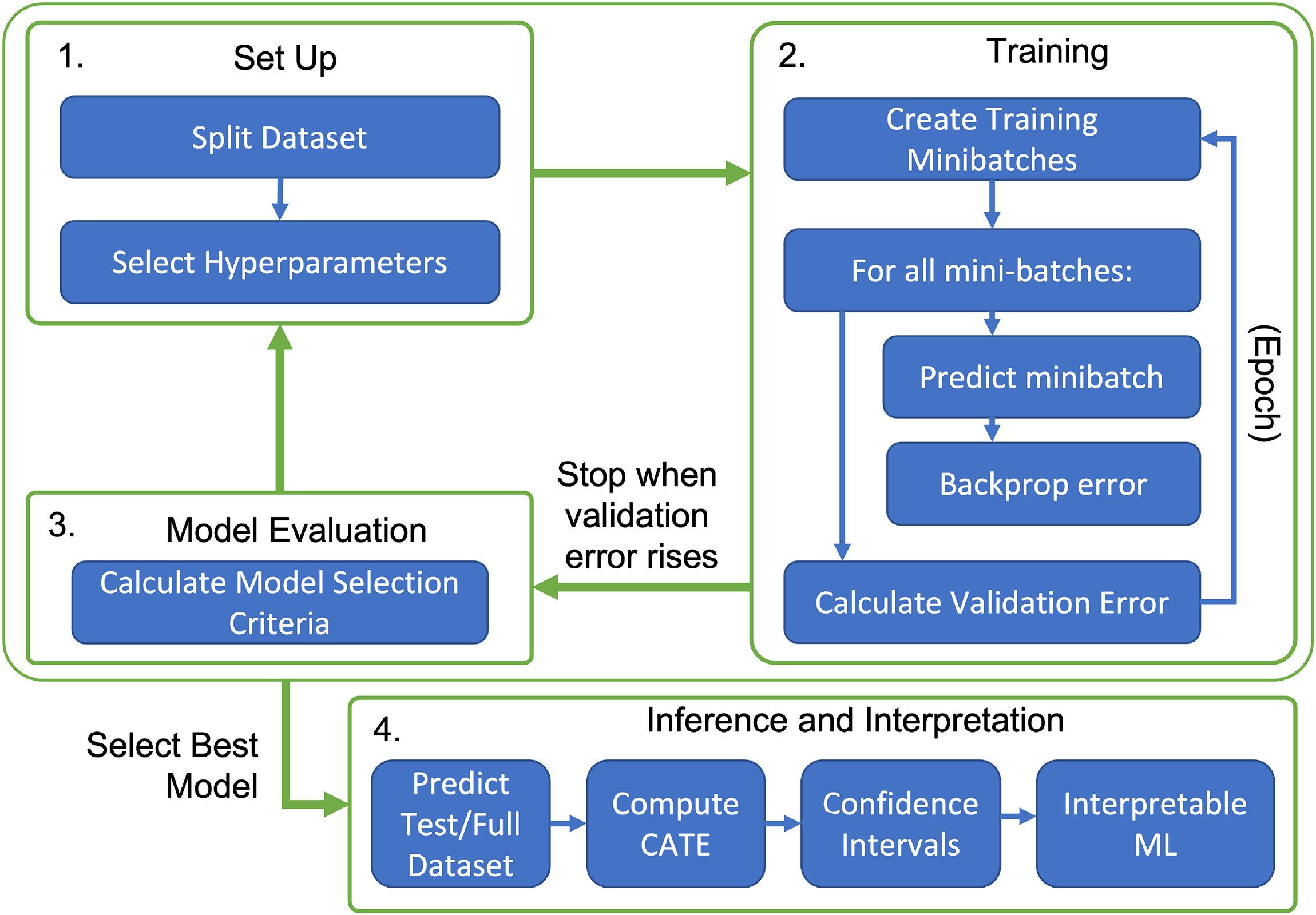
Diagnosing and addressing overfitting is a more challenging problem. In supervised learning, overfitting is diagnosed after training (but before testing) by assessing predictive performance in a reserved portion of the training set called the validation set. If the model fits the training dataset well but performs poorly in the validation set, it is likely to generalize poorly to the test set as well. To prevent overfitting, regularization techniques can be used to simplify the complexity of the model. Training and regularization of neural networks is discussed in detail in the “Deep Learning in Practice” section. For a full treatment of supervised learning and statistical learning theory, see Hastie, Tibshirani, and Friedman (2009).

Figure 2.

Supervised Deep Learning Workflow. (1) Set Up: The first step in training a deep learning model is splitting the data into a training set, validation set, and optionally a test set. Initial hyperparameters are then selected from a set of choices specified by the user. (2) Training: In each iteration of the training process (called an epoch), the training set is randomly divided into small minibatches For each minibatch, the network makes predictions for all units, and calculates the error gradients to be assigned to each neuron in the network based on those predictions. An optimizer then moves the network’s parameters in the opposite direction of the error gradient. After all minibatches have been trained (one epoch), error is calculated on the entire validation set. This whole process is repeated up until the validation error stops decreasing (to avoid overfitting). (3) Model Evaluation: A criterion (typically the validation error) is used to evaluate the performance of this hyperparameterization. New hyperparameters are then selected using a hyperparameter optimization algorithm (eg. Grid search, Bayesian hyperparameter optimization, genetic algorithms) and steps 1 and 2 are repeated. Once the hyperparameter optimization algorithm has completed its search, the “best” model is selected for inference. (4) Inference and interpretation: With a model selected, the analyst is now ready to apply it to their test data (or in the case of statistical inference, potentially the full dataset). Predictions of the outcomes and/or propensity score can then be used to compute the CATE (conditional average treatment effect) and calculate confidence intervals. Feature importance algorithms like SHapley Additive exPlanations (SHAP) or Integrated Gradients can also be used to interpret the CATE estimates.

Set Up and Hyperparameters

The first step in training a neural network, as in other types of supervised ML, is to split your dataset into training, validation, and testing datasets (Figure 2A). If the network is being used for statistical inference, as here, the testing dataset is optional, and inference may be conducted on just the validation set or the full dataset.

While the computational graph and loss function define a deep learning architecture (Box 3), actual implementations can vary significantly due to the choice of hyperparameters. In supervised ML, hyperparameters are parameters that are not learned automatically when training the model but must be specified by the analyst. In deep learning, architectural hyperparameters include the number of layers to use for each section of the computational graph, the number of neurons to use in each layer, and the activation functions to be used by neurons. While some basic rules of thumb apply (e.g., use fewer layers than neurons), these choices remain poorly understood theoretically⁴ ; decisions are generally made by comparing empirical performance on the validation set, a practice called hyperparameter tuning. Box 3:

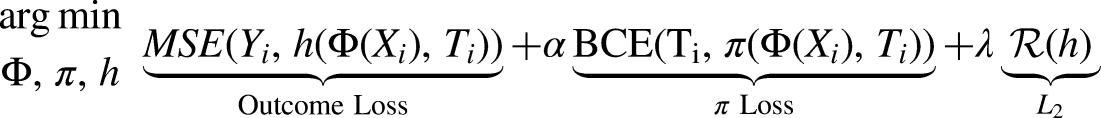
Reading Machine Learning Papers: Computational Graphs and Loss Functions

Within the machine learning literature, novel algorithms are often presented in terms of their computational graph and loss function. A computational graph (not to be confused with a causal graph) uses arrows to depict the flow of data from the inputs of a neural network, through parameters, to the outputs. Layers of neurons or specialized sub-architectures are often generically abstracted as shapes. In our diagrams, we use rounded purple shapes to represent observables, orange rectangles for representation layers of the network, rounded white shapes for produced outputs, and textured rectangles for outcome modeling layers. Operations that are computed after prediction (i.e., for which an error gradient is not calculated) are shown with dashed lines (e.g., plug-in estimation of causal estimands).

Figure 1.

A: Generalized linear model (GLM) represented as a computational graph. Observable covariates $X_{1}, X_{2}, X_{3}$ and treatment status $T$ depicted in rounded purple boxes. Each of the lines between the rounded purple inputs and the textured box represents a parameter (i.e., a $β$ in a GLM equation). The textured box is an “output neuron” that sums its weighted inputs, performs a transformation $g$ (the link function in GLM; in this case the identity function), and predicts the conditional outcome $\hat{Y} (T)$ . Instead of theoretically interpreting these parameters from an inferential statistics perspective, ML approaches typically use the predicted observed and unobserved potential outcomes for plug-in estimation of causal estimands (e.g., the $\hat{C A T E}$ ). After training, setting $T$ to $1 - T$ for each observation can predict the unobserved potential outcome $\hat{Y} (1 - T)$ . Because this operation occurs after prediction and does not feed a gradient back to the network to optimize the parameters, it is depicted here with a dotted line. Plug-in calculation of $\hat{C A T E}$ is similarly shown with a dotted line. B: Feed-forward neural network (S-learner). In a feed-forward neural network, additional fully connected (parameterized) layers of neurons are added between the inputs (rounded purple) and output neuron. The size of the input covariates and hidden layers are generically abstracted as boxes (orange). The final hidden layer before the output neuron is denoted $Φ$ because the hidden layers collectively encode a representation function (see the “Representation Learning and Multitask Learning” section). In causal inference settings, this architecture is sometimes called as S(ingle)-learner because one feed-forward network learns to predict both potential outcomes.

Along with the architecture, the loss function of a neural network is the primary means for the analyst to dictate what types of representations a neural network learns and what types of outputs it produces. In multitask learning settings, we denote joint loss functions for an entire network as a weighted sum of the losses for constituent tasks and modules. These specific losses are weighted by hyperparameters. For example, we might weight the joint loss for a network that predicts outcomes and propensity scores as: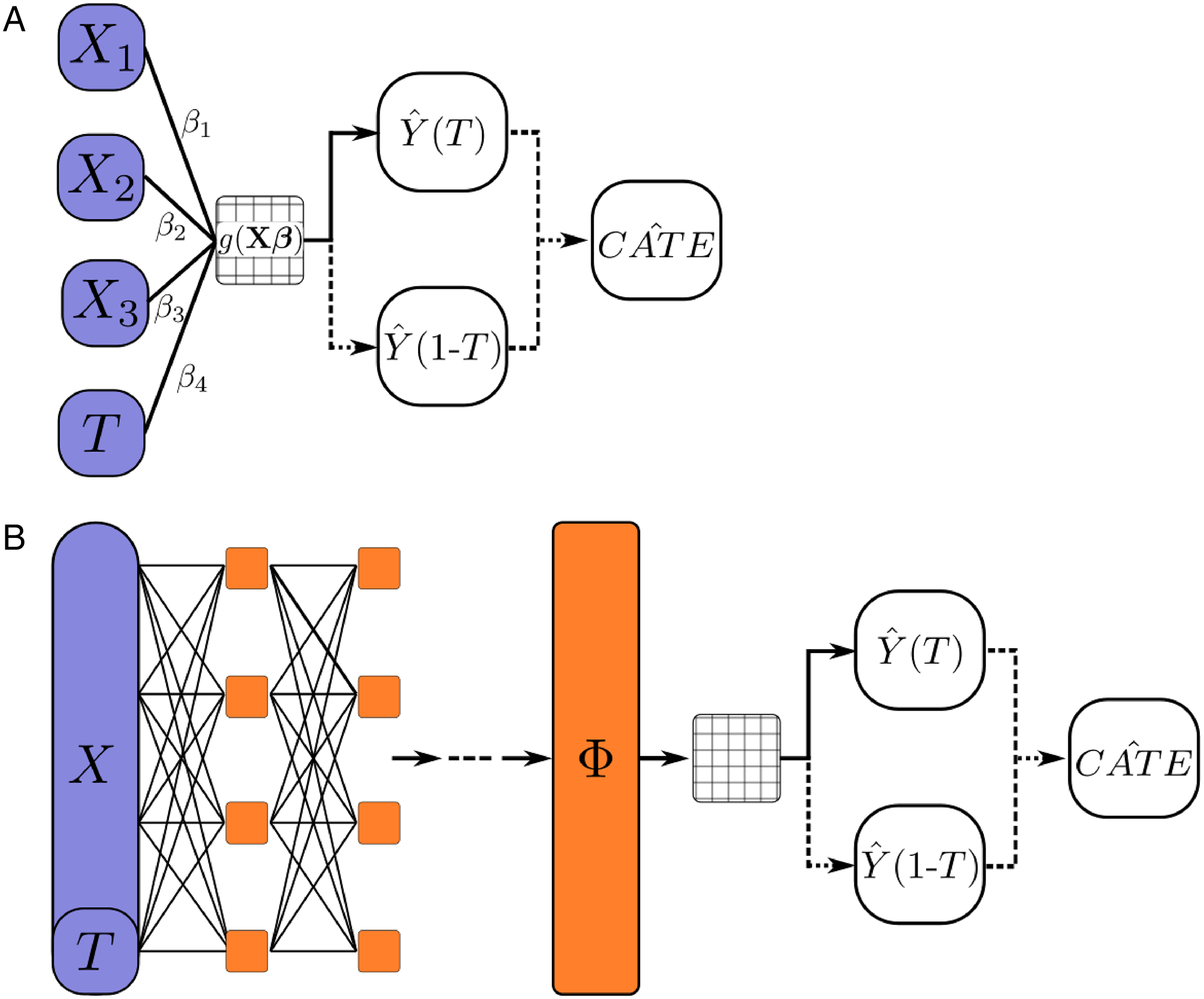

\binom{\arg \min}{h, π} L = L_{h} + λ L_{π} = M S E (Y, h (X, T)) + λ B C E (T, π (X, T))

where

h (X, T)

is the predicted potential outcome,

π (X, T)

is the predicted propensity score,

λ

is a hyperparameter and MSE and BCE stand for mean squared error and binary cross entropy (i.e., log loss), common losses for regression and binary classification respectively (Box 6).

Training and Regularization

Neural networks are trained by repeatedly making predictions from the training set, calculating error gradients for each parameter, and backpropagating small fractions of those error gradients. (Figure 2 B). A full pass-through examples in the training set is called a training loop or epoch. At the beginning of each epoch, the training set is divided into mini-batches of 2 to 1024 units, randomly sampled without replacement. This practice not only aids in memory management, it also improves optimization. Using small random samples effectively introduces noise into the training process, making it less likely for the model to get stuck in local minima.

The size of mini-batches can be considered a hyperparameter.⁵ Because a mini-batch of data is only a sample of a sample (the training dataset), the optimizer only adjusts weight parameters by a fraction of the error gradient (the learning rate) to avoid overfitting. The learning rate is also a hyperparameter, which typically varies between 0.0001 and 0.01.

The nonconvex nature of most loss functions⁶ mean that optimization often requires hundreds to potentially millions of epochs of training. Moreover, neural networks are highly susceptible to overfitting because it is easy to overparameterize them with excessive neurons/layers. To ward against overfitting, error metrics on the complete validation set are computed at the end of every epoch. In a regularization practice called “early stopping,” analysts usually stop training once validation metrics stop improving. Other common regularization techniques include weight decay (i.e., $ℓ^{2}$ norm, ridge, or Tikhonov) penalties on the parameters, dropout of neurons during training, and batch normalization.

Dropout is a regularization technique in deep learning where certain nodes are randomly silenced from training during a given epoch (Srivastava et al., 2014). The general idea of dropout is to force two neurons in the same layer to learn different aspects of the covariate/feature space and reduce overfitting. Batch normalization is another regularization technique applied to a layer of neurons (Ioffe and Szegedy, 2015). By standardizing (i.e. z-scoring) the inputs to a layer on a per-batch basis and then rescaling them using trainable parameters, batch normalization smooths the optimization of the loss function. The addition and extent of each of these regularization techniques can be treated as hyperparameters.

Model Selection

(Tutorial 2 )

After the model has been trained, the analyst compares models assembled with different hyperparameterizations or initial parameter values (Figure 2C). Hyperparameterizations can be chosen using random search, an exhaustive grid search of all possible combinations, or strategic search algorithms like Bayesian hyperparameter optimization or evolutionary optimization (Snoek, Larochelle, and Adams, 2012). Validation loss metrics on the final epoch are commonly used for these comparisons.

Model selection for causal estimators is complicated by the fundamental problem of causal inference: we are not actually interested in the observed “factual” outcomes and propensity scores, but the CATE and ATE (average treatment effect). In the case of algorithms like Dragonnet where the validation loss explicitly targets a causal quantity, we use that as the model selection criterion. In cases where the algorithm is only trained for outcome modeling or propensity modeling, other solutions are needed. In the Online Appendix, we describe Johansson et al. (2020)’s proposal to use matching on a nearest neighbor approximation of the Precision in Estimated Heterogeneous Effects (PEHE), a measure of CATE bias, as an alternative model selection metric (Online Appendix A).

The development of more sophisticated methods for model selection of causal estimators through data simulation is an active area of research within this literature.⁷ For example, Parikh et al. (2022) use deep generative models to approximate the data generating distribution under weak, nonparametric assumptions. Alaa and Van Der Schaar (2019) independently model each outcome and the propensity score before using influence functions to assess model error.

Representation Learning and Multitask Learning

One comparative advantage of deep learning over other ML approaches has been the ability of ANNs to encode and automatically compress informative features from complex data into flexible, relevant “representations” or “embeddings” that make downstream supervised learning tasks easier (Goodfellow, Bengio, and Courville, 2016; Bengio, 2013). While other ML approaches may also encode representations, they often require extensive preprocessing to create useful features for the algorithm (i.e., feature engineering). Through the lens of representation learning, a geometric interpretation of the role of each layer in a supervised neural network is to transform its inputs (either raw data or output of previous layers) into a typically lower (but possibly higher) dimensional vector space. As a means to share statistical power, encoded representations can also be jointly learned for two tasks at once in multitask learning.

The simplest example of a representation might be the final layer in a feed-forward network, where the early layers of the network can be understood as nonlinearly encoding the inputs into an array of latent linear features for the output neuron (Goodfellow, Bengio, and Courville, 2016) (Figure 1B). A famous example of representation learning is the use of neural networks for face detection. Examining the representations produced by each layer of these networks shows that each subsequent layer seems to capture increasingly abstract features of a face (first edges, then noses and eyes, and finally whole faces) (LeCun, Bengio, and Hinton, 2015). A more familiar example of representation learning to social scientists might be word vector models like Word2Vec (Mikolov et al., 2013). Word2Vec is a neural network with one hidden layer and one output layer where words that are semantically similar are closer together in the representation space created by the hidden layer of the network.

The novel contribution of deep learning to causal estimation is the proposal that a neural network can learn a function $Φ$ that produces representations of the covariates decorrelated from the treatment. Fundamentally, the idea is that $Φ$ can transform the treated and control covariate distributions into a representation space such that they are indistinguishable (Figure 3). To ensure that these representations are also still predictive of the outcome (multitask learning), multiple loss functions are generally applied simultaneously to balance these objectives. This approach is applied in a majority of the algorithms presented in the “Three Different Approaches to Deep Causal Estimation” section.

Figure 3.

Balancing through representation learning. The promise of deep learning for causal inference is that a neural network encoding function $Φ$ can transform the treated and control covariate distributions into a representation space such that they are indistinguishable. Used with permission from Johansson and Shen (2018).

Causal Identification and Estimation Strategies

Identification of Causal Effects

The papers described in this primer are primarily framed within the Potential Outcomes causal framework (Neyman-Rubin causal model) (Rubin, 1974; Imbens and Rubin, 2015). This framework is concerned with identifying the “potential outcomes” of each unit $i$ in the sample, had it received treatment ( $Y (1)$ ) or not received treatment ( $Y (0)$ ). However, because each unit can only receive one treatment regime in reality (being treated or remaining untreated), it is not possible to observe both potential outcomes for each individual (often termed “the fundamental problem of causal inference”) (Holland, 1986). While we cannot thus identify individual treatment effects $τ_{i} = Y_{i} (1) - Y_{i} (0)$ for each unit, causal inference frameworks allow us to probabilistically estimate average treatment effects ( $A T E s$ ) and ATEs conditional on select covariates ( $C A T E$ ) across samples of treated and control units. Within this literature, the motivation of many papers is to present algorithms that can both infer CATEs from observational data, but also predict them for out-of-sample units where treatment status is unknown. For readers unfamiliar with causal inference, a short introduction is glossed in Box 4 with a concrete example, used in the tutorials, in Box 5. Box 4:

Basic Introduction to Causal Inference

Correlation does not equal causation, and causal inference is concerned with the identification of causal relationships between random variables. Many causal questions we would like to ask about social data (What is the causal effect of $T$ on $Y$ for units with characteristics $X$ ?) can be unpacked as counterfactual questions with the general format: “What would have been the outcome $Y$ for a unit with $X$ characteristics, if $T$ had happened or not happened?”.

Randomized control trials (RCTs, also known as A/B testing in data science and industry applications) are usually understood to be the ideal approach to answering this type of question: each unit with covariates or features $X$ is randomly assigned to the treatment or control groups and outcome $Y$ is subsequently measured. But in many scenarios, it is prohibitively expensive or unethical (e.g., randomly assigning students to attend college or not) to collect experimental data. In these cases, we can statistically adjust observational data (e.g., survey data on college attendance) to approximate the experimental ideal. The methods described in this paper are designed to answer counterfactual questions with primarily nonexperimental observational data.

There are at least three different schools of causal inference that have been introduced in social statistics and econometrics (Rubin, 1974; Imbens and Rubin, 2015), epidemiology (Robins, 1986, 1987; Hernán and Robins, 2020), and computer science (Goldszmidt and Pearl, 1996; Pearl, 2009). The goal of these causal frameworks is to describe and correct for biases in data or study design that would prevent one from making a true causal claim. If these biases are correctable and the causal effect can be uniquely expressed in terms of the distribution of observed data, then we say that the causal effect is identifiable (Kennedy, 2016). Only if a causal effect is identifiable can we use statistical tools to correct for biases and estimate the causal effect (e.g., inverse propensity score weighting, g-computation, deep learning).

The algorithms presented in this paper focus on estimating causal effects primarily by correcting for confounding bias. Loosely speaking, a confounding covariate/feature is one that is correlated with both the treatment and the outcome, misleadingly suggesting that the treatment has a causal effect on the outcome, or obscuring a true causal relationship between the treatment and outcome. Often times, the confounder is a cause of the treatment and outcome. As an example of confounding bias, estimating the causal effect of attending college (treatment) on adult income (outcome) requires controlling for the fact that parental income may be a common cause of both college attendance and adult income.

Box 5:

Applied Causal Inference Example: The Infant Health and Development Study

To make this problem setting more concrete for readers unfamiliar with causal inference, consider simulations based on the 1985–1988 Infant Health and Development Study that are widely used as benchmarks within this literature. In this experiment, premature children were randomly assigned to intensive, high-quality childcare ( $T$ ), and their cognitive test scores were measured later ( $Y$ ). The authors also measured numerous other covariates $X$ including “pregnancy complications, child’s birth weight and gestation age, birth order, child’s gender, household composition, day care arrangements, source of health care, quality of the home environment, parents’ race and ethnicity, and maternal age, education, IQ, and employment” (Ramey et al., 1992). The $A T E$ would be the effect of intensive child care on cognitive scores across all children, while various $C A T E$ s might be formulated to better understand how the effects of child care vary for female children, children born to teenage mothers, or children with unemployed parents.

Hill (2011) turns this experimental data into an observational benchmark by re-simulating the outcome such that the covariates $X$ induce confounding bias between the treatment and outcome. While the simulations don’t preserve the names of the covariates, we can imagine some confounding relationships that might be present in an observational study. For example, suppose that affluent ( $X_{1}$ ) parents are more likely able to afford high-quality child care ( $T$ ), but there is actually a weak association between childcare and premature babies’ cognitive ability ( $Y$ ). We also know affluent parents are more likely to engage in breastfeeding ( $X_{2}$ ), which is positively associated with higher cognitive ability (Heck et al., 2006; Kramer et al., 2008). If we do not account for the correlation between income and childcare ( $X_{1} \to T$ ), or income and cognitive ability ( $X_{1} \to X_{2} \to Y$ ), we may have bias in our $A T E$ / $C A T E$ estimates, or worse, erroneously interpret the correlation between childcare and cognitive ability as causal. This example is depicted in a causal graph below.

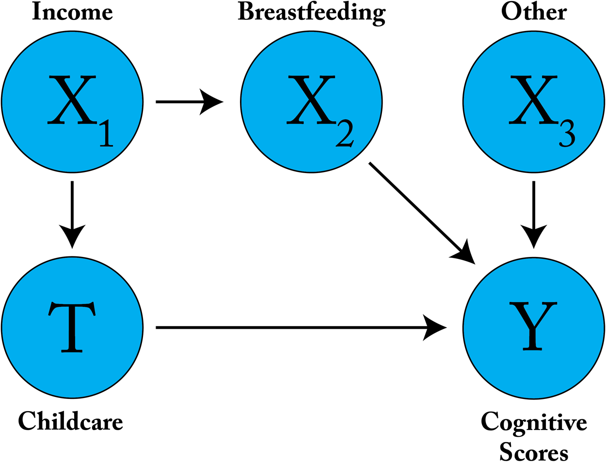
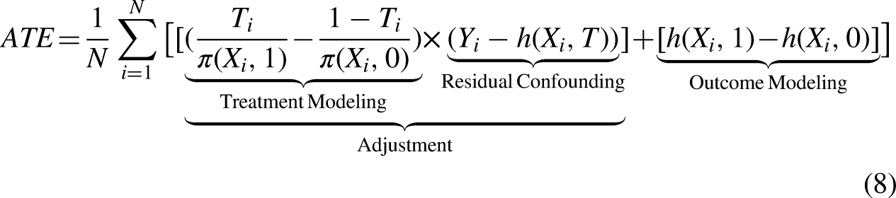
The hypothetical confounding bias presented here can be adjusted for either through treatment modeling (e.g., inverse propensity score weighting, nonparametric, deep representation learning) to block the path $X_{1} \to T$ , outcome modeling (e.g., generalized linear models, deep regression) to block the path $X_{1} \to X_{2} \to Y$ , or both (see the “Estimation of Causal Effects” section). For coded examples using the IHDP benchmark, see the tutorials.

The ATE is defined as:

A T E = E [Y (1) - Y (0)] = \frac{1}{N} \sum_{i} (Y_{i} (1) - Y_{i} (0)) = \frac{1}{N} \sum_{i} τ_{i} = E [τ]

where

Y_{i} (1)

and

Y_{i} (0)

are the potential outcomes had the unit

i

received or not received the treatment, respectively. The CATE is defined, with a slight but heuristic abuse of notation, as,

C A T E (x) = E [Y_{i} (1) - Y_{i} (0) | X_{i} = x] = E [τ_{i} | X_{i} = x] = \frac{1}{N} \sum_{i | X_{i} = x} τ_{i}

where

X

is the set of selected, observable covariates,

x \in X

represents particular values of those covariates, and we condition on

X_{i} = x

to indicate that the expectation is taken only over units

i

with covariates

X_{i} = x

Within the ML literature on causal inference treated here, the primary strategy for causal identification is selection on observables. A challenge to identifying causal effects is the presence of confounding relationships between covariates associated with both the treatment and the outcome.

The key assumptions allowing the identification of causal effects in the presence of confounding are:

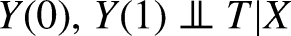
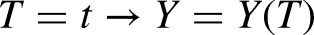
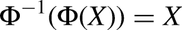
Conditional Ignorability/Exchangability The potential outcomes $Y (0)$ , $Y (1)$ and the treatment $T$ are conditionally independent given $X$ ,

Y (0), Y (1) ⊥ ⊥ T | X

Conditional Ignorability specifies that there are no unmeasured confounders that affect both treatment and outcome outside of those in the observed covariates/features

X

. Additionally,

X

may contain predictors of the outcome (helping precision), but should not contain instrumental variables (hurting precision and potentially amplifying residual bias) or colliders within the conditioning set.⁸

Other standard assumptions invoked to justify causal identification are:

Consistency/Stable Unit Treatment Value Assumption (SUTVA). Consistency specifies that when a unit receives treatment, their observed outcome is exactly the corresponding potential outcome (and the same goes for the outcomes under the control condition). Moreover, the response of any unit does not vary with the treatment assignment to other units (i.e., no network or spillover effects), and the form/level of treatment is homogeneous and consistent across units (no multiple versions of the treatment). Note that this is an identification assumption, based on our understanding of the data-generating process, and independent of the model chosen for estimation. More formally,

T = t \to Y = Y (T)

Overlap. For all $x \in X$ (i.e., any observed covariate value), all treatments $t \in {0, 1}$ have a nonzero probability of being observed in the data, within the “strata” defined by such covariates,

1 > p (T = t | X = x) > 0

An additional assumption sometimes invoked at the interface of identification and estimation using neural networks is:

Invertability

Φ^{- 1} (Φ (X)) = X

In other words, there must exist an inverse function of the representation function

Φ

encoded by a neural network that can reproduce

X

from representation space. This is required for the Conditional Ignorability assumption to hold when using representation learning. From a practical perspective, it also means that the representation we created is rich enough to capture the causal relationships we are interested in.

For reference, we describe the full notation used within the primer in Box 6.

Box 6:

Notation for Causal Inference and Estimation

We use uppercase to denote general quantities (e.g., random variables) and lowercase to denote specific quantities for individual units (e.g., observed variable values).

Causal identification

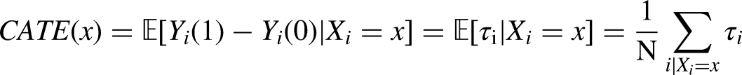
Observed covariates/features: $X$

Potential outcomes: $Y (0)$ and $Y (1)$

Treatment: $T$

Unobservable Individual Treatment Effect: $τ_{i} = Y_{i} (1) - Y_{i} (0)$

Average treatment effect: $A T E = E [Y (1) - Y (0)] = E [τ]$

Conditional average treatment effect: $C A T E (x) = E [Y_{i} (1) - Y_{i} (0) | X_{i} = x] = E [τ_{i} | X_{i} = x]$

Deep learning estimation

Predicted potential outcomes: $\hat{Y} (0)$ and $\hat{Y} (1)$

Outcome modeling functions: $\hat{Y} (T) = h (X, T)$

Propensity score function: $π (X, T) = P (T | X)$ (where $π (X, 0) = 1 - π (X, 1)$ )

Representation functions: $Φ (X)$ (producing representations $ϕ$ )

Loss functions: $L (t r u e, p r e d i c t e d)$

Loss abbreviations: $M S E$ (mean squared error), $B C E$ (binary cross-entropy), CCE (categorical cross-entropy)

Loss hyperparameters: $λ, α, β$

Estimated CATE* for unit $i$ with covariates $X_{i}$ : $\hat{C A T E_{i}} = {\hat{τ}}_{i} = \hat{Y_{i}} (1) - \hat{Y_{i}} (0) = h (X_{i}, 1) - h (X_{i}, 0)$

Estimated ATE: $\hat{A T E} = \frac{1}{N} \sum_{i = 1}^{N} \hat{τ_{i}}$

Beyond the

A T E

and

C A T E

there is an additional metric commonly used in the machine learning literature, first introduced by Hill (2011) called the Precision in Estimated Heterogeneous Effects (PEHE) . PEHE is the average error across the predicted

C A T E

Precision in Estimated Heterogeneous Effects: $P E H E = \frac{1}{N} \sum_{i = 1}^{N} (τ_{i} - \hat{τ_{i}})^{2}$

Beyond being a metric for simulations with known counterfactuals, the

P E H E

has theoretical significance in the formulation of generalization bounds within this literature (Shalit, Johansson, and Sontag, 2017; Johansson et al., 2018, 2020; Zhang, Bellot, and Schaar, 2020).

*Note that we use $\hat{τ}$ to refer to the estimated CATE because truly individual treatment effects cannot be described only by the observed covariates $X$ .

Estimation of Causal Effects

Once a strategy for identifying causal effects from available data has been developed (arguably the harder and more important part of causal inference), statistical methods can be used to estimate causal effects by controlling for confounding bias, selection bias, and/or measurement error. 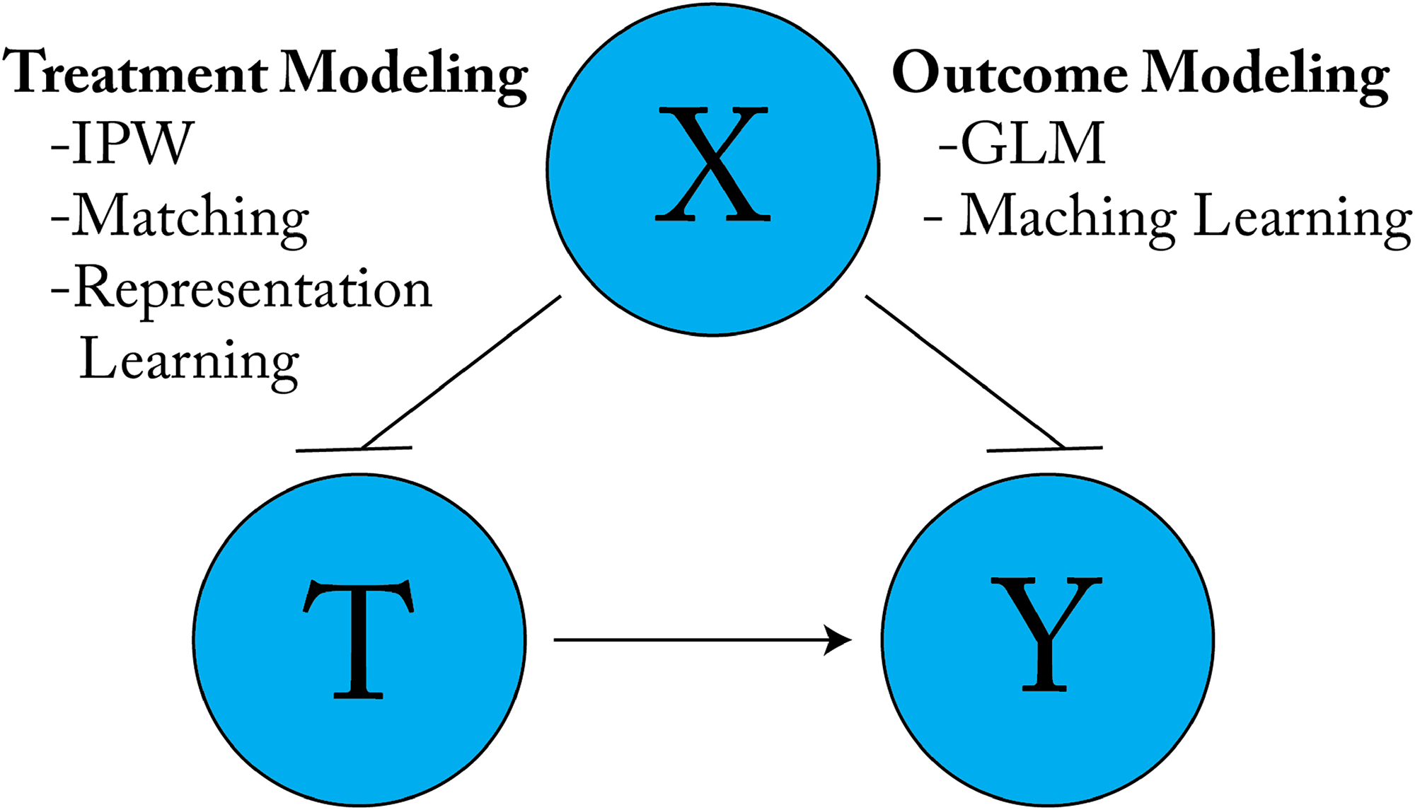There are two fundamental approaches to estimation: treatment modeling to control for correlations between the covariates $X$ and the treatment $T$ , and outcome modeling to control for correlations between the covariates $X$ and the outcome $Y$ (Figure 4). Below we briefly review three traditional techniques for removing confounding bias to motivate our systematization of deep learning models. First, we discuss outcome modeling through regression. Next, we consider treatment modeling through nonparametric matching. Finally, we discuss treatment modeling through IPW and introduce the concept of double robustness.

Figure 4.

Two fundamental approaches to deconfounding. Blunted arrows indicate blocked causal paths. Treatment modeling approaches like inverse propensity weighting, balancing, and representation learning adjust for the association between the covariates $X$ and the treatment $T$ . Outcome modeling approaches like generalized linear models or machine learning regressors adjust for the association between $X$ and the outcome $Y$ .

Outcome Modeling: Regression

Assuming the treatment effect is constant across covariates/features or the probability of treatment is constant across all covariates/features (both improbable assumptions), the simplest consistent approach to estimating the $A T E$ is to regress the outcome on the treatment indicator and covariates using a linear model.⁹ The ATE is then the coefficient of the treatment indicator. Without loss of generality, we call outcome models of this nature, linear or nonlinear, $h$ :

{\hat{Y}}_{i} (T) = h (X_{i}, T)

A slightly more sophisticated semiparametric approach to outcome modeling, used widely in the application of ML to causal inference, is to use

h (X, T)

to impute

\hat{Y} (1)

and

\hat{Y} (0)

, and calculate the CATE for each unit as a plug-in estimator:

\hat{C A T E_{i}} = \hat{τ_{i}} = \hat{Y_{i} (1)} - \hat{Y_{i} (0)} = h (X_{i}, 1) - h (X_{i}, 0)

and the ATE as:

\hat{A T E} = \frac{1}{N} \sum_{i = 1}^{N} \hat{τ_{i}}

Treatment Modeling: Nonparametric Matching

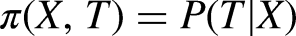
A common treatment-modeling strategy is balancing the treated and control covariate distributions through matching. Matching requires the analyst to select a distance measure that captures the difference in observed covariate distributions between a treated and untreated unit (Austin, 2011). Units with treatment status $T$ can then be matched with one or more counterparts with treatment status $1 - T$ using a variety of algorithms (Stuart, 2010). In a one-to-one matching scenario where each treated unit has an otherwise identical untreated counterpart, the covariate distribution of treated and control units is indistinguishable.

Treatment Modeling: IPW

Another common approach is IPW. In IPW, units are weighted on their inverse propensity to receive treatment. Without loss of generality, we call the propensity function $π$ . The propensity score is calculated as the probability of receiving treatment conditional on covariates:

π (X, T) = P (T | X)

The simplest IPW estimator of the ATE is then:

\hat{A T E} = \frac{1}{N} \sum_{i = 1}^{N} [\frac{T_{i} Y_{i}}{\hat{π} (X_{i}, 1)} - \frac{(1 - T_{i}) Y_{i}}{\hat{π} (X_{i}, 0)}]

(1)

Note that only one of the two terms is active for any given unit. Furthermore, this presentation looks different than how the IPW is generally presented because we use

π

as a function with different outputs depending on the value of

T

rather than a scalar (Box 6).¹⁰

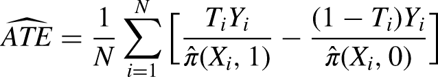
IPW weighting is attractive because if the propensity score $π$ is specified correctly, Equation 1 is an unbiased estimator of the ATE. Moreover, the IPW is consistent if $π$ is estimated consistently (Rosenbaum and Rubin, 1983; Glynn and Quinn, 2010).

Double Robustness

Because different models make different assumptions, it is not uncommon to combine outcome modeling with propensity modeling or matching estimators to create doubly robust estimators. For example, one of the most widely used doubly robust estimators is the augmented-IPW estimator.

\hat{A T E} = \frac{1}{N} \sum_{i = 1}^{N} [\underset{Adjustment}{\underset{⏟}{\underset{Treatment \,\,Modeling}{\underset{⏟}{[\frac{T_{i}}{π (X_{i}, 1)} - \frac{1 - T_{i}}{π (X_{i}, 0)}]}} \times \underset{Residual \,\,Confounding}{\underset{⏟}{[Y_{i} - h (X_{i}, T_{i})]}}}} + \underset{Outcome \,\,Modeling}{\underset{⏟}{[h (X_{i}, 1) - h (X_{i}, 0)]}}]

(2)

The first term is a “corrected” IPW estimator replacing the raw outcome by the residuals from the regression models while the second term is the difference in prediction from two outcome models, one for treated and one for control units. As expected, this estimator is unbiased if the IPW and regression estimators are consistently estimated. However, the model is attractive because it will be consistent if either the propensity score

π (X, T)

is correctly specified or the regression model

h

is consistently specified (Glynn and Quinn, 2010). The model also provides efficiency gains with respect to the use of each model separately, and especially with respect to weighting alone.

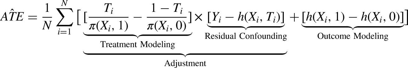
Doubly robust estimation is especially important for causal estimation using ML. When using simple outcome plug-in estimators, bias is directly dependent on estimation error, which may be different for each potential outcome depending on the modeling strategy (Kennedy, 2020). ML estimation of the propensity score can also rely heavily on nonconfounding predictors, giving rise to extreme weights (Schnitzer, Lok, and Gruber, 2016). More generally, there are no asymptotic linearity guarantees for ML estimators which may converge at a slow rate, leading to misleading confidence intervals (Naimi, Mishler, and Kennedy, 2021; Zivich and Breskin, 2021). For these reasons, plug-in ML estimation often has poor empirical performance when not using double robust estimators (Benkeser et al., 2017; Kennedy, 2020; Zivich and Breskin, 2021).

The growth of ML for causal inference literature has thus been largely driven by the introduction of semiparametric frameworks. Semiparametric frameworks address these issues by using ML only to estimate the nuisance parameters (i.e., potential outcomes and propensity score) of influence functions for causal parameters like the ATE and CATE (Chernozhukov et al., 2018; Kennedy, 2016; Van der Laan and Rose, 2011). In these approaches, the estimation of causal parameters is only second order dependent on ML error, there is double-robustness against inconsistent estimation, and guarantees of fast convergence and asymptotically valid confidence intervals even if the ML models converge slowly (Benkeser et al., 2017; Kennedy, 2020; Naimi, Mishler, and Kennedy, 2021; Zivich and Breskin, 2021). We use the final algorithm introduced below, Dragonnet, as an opportunity to provide an intuitive introduction to semiparametric theory and how it can be used for doubly robust estimation (Shi, Blei, and Veitch, 2019).

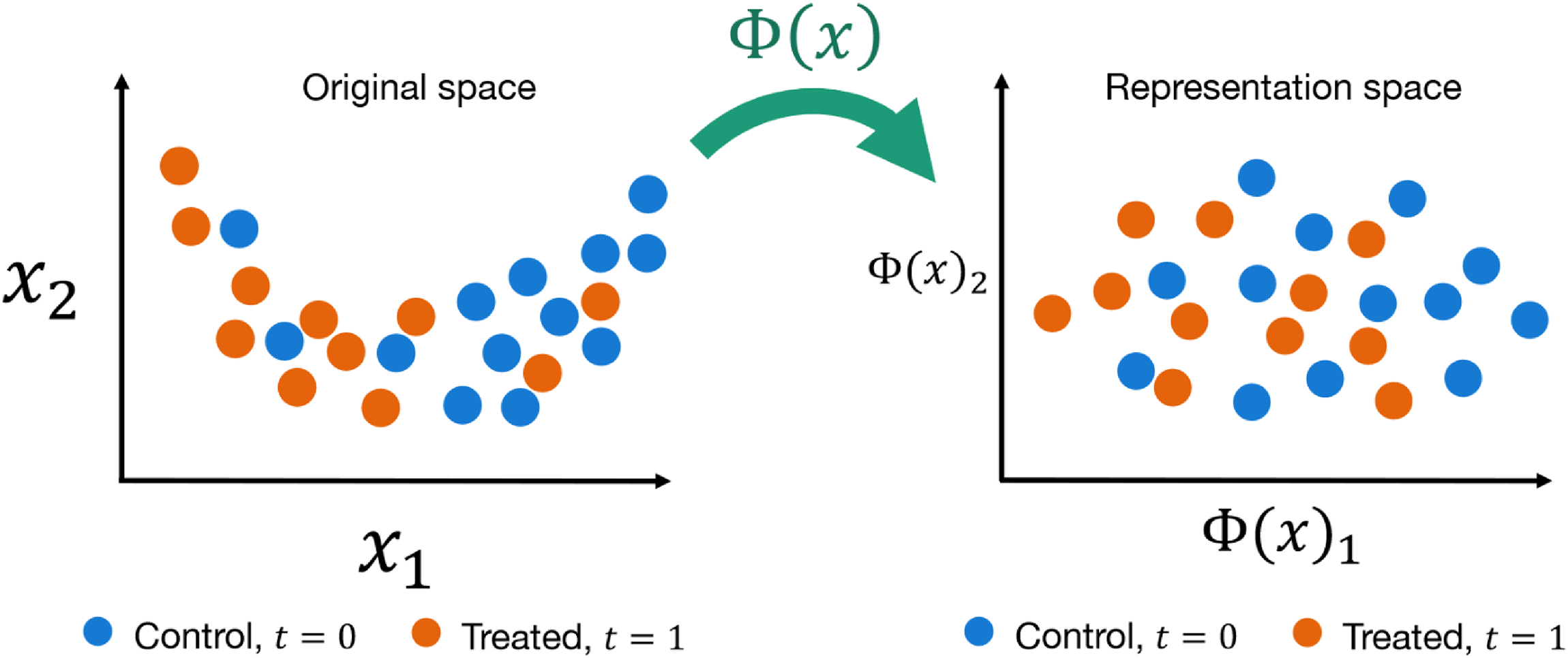
Three Different Approaches to Deep Causal Estimation

The architectures proposed in the deep learning literature for causal estimation build upon the core idea discussed above. First, we introduce “S-Learners” and “T-Learners” to show how neural networks can be used to estimate nonlinearities in potential outcomes. Second, given the right objectives, a neural network can learn representations of the treated and control distributions that are deconfounded (Figure 3). This approach, which can be related theoretically to nonparametric matching, is illustrated by the foundational TARNet algorithm in the “Double Robustness with IPW” section (Shalit, Johansson, and Sontag, 2017). Finally, the ML for causal inference literature has been largely driven by the introduction of semiparametric frameworks that allow predictive ML models to be plugged-in to doubly robust estimation equations (Van der Laan and Rose, 2011; Chernozhukov et al., 2018, 2021). In the “Double Robustness with IPW” section, we introduce the concept of influence functions and the targeted maximum likelihood estimator to explain the Dragonnet algorithm. For clarity, the algorithms presented here all share a familial resemblence to the TARNet algorithm. However, we note that there are many other approaches to using deep learning for causal inference (e.g., the generative models described in Online Appendix).

Deep Outcome Modeling

S-Learners and T-Learners (Tutorial 1 )

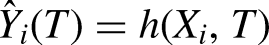
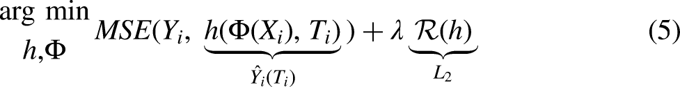
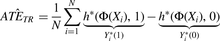
Because at most one potential outcome is unobserved, it is not possible to apply supervised models to directly learn treatment effects. Across econometrics, biostatistics, and ML, a common approach to this challenge has been to instead use ML to model each potential outcome separately and use plug-in estimators for treatment effects (Chernozhukov et al., 2018; Van der Laan and Rose, 2011; Wager and Athey, 2018). As with linear models, a single neural model can be trained to learn both potential outcomes (S[ingle]-learner) (Figure 1B), or two independent models can be trained to learn each potential outcome (a “T-learner”) (Johansson et al., 2020) (Figure 5A). In both cases, the neural network estimators would be feed-forward networks tasked with minimizing the MSE in the prediction of observed outcomes. In a slight abuse of notation, the joint loss function for a T-learner can be written as:

L (Y, h (X, T)) = M S E [Y_{i}, T_{i} \times h_{1} (X_{i}, 1) + (1 - T_{i}) \times h_{0} (X_{i}, 0)]

(3)

where

h_{1}

and

h_{0}

represent separate networks for each potential outcome.

Figure 5.

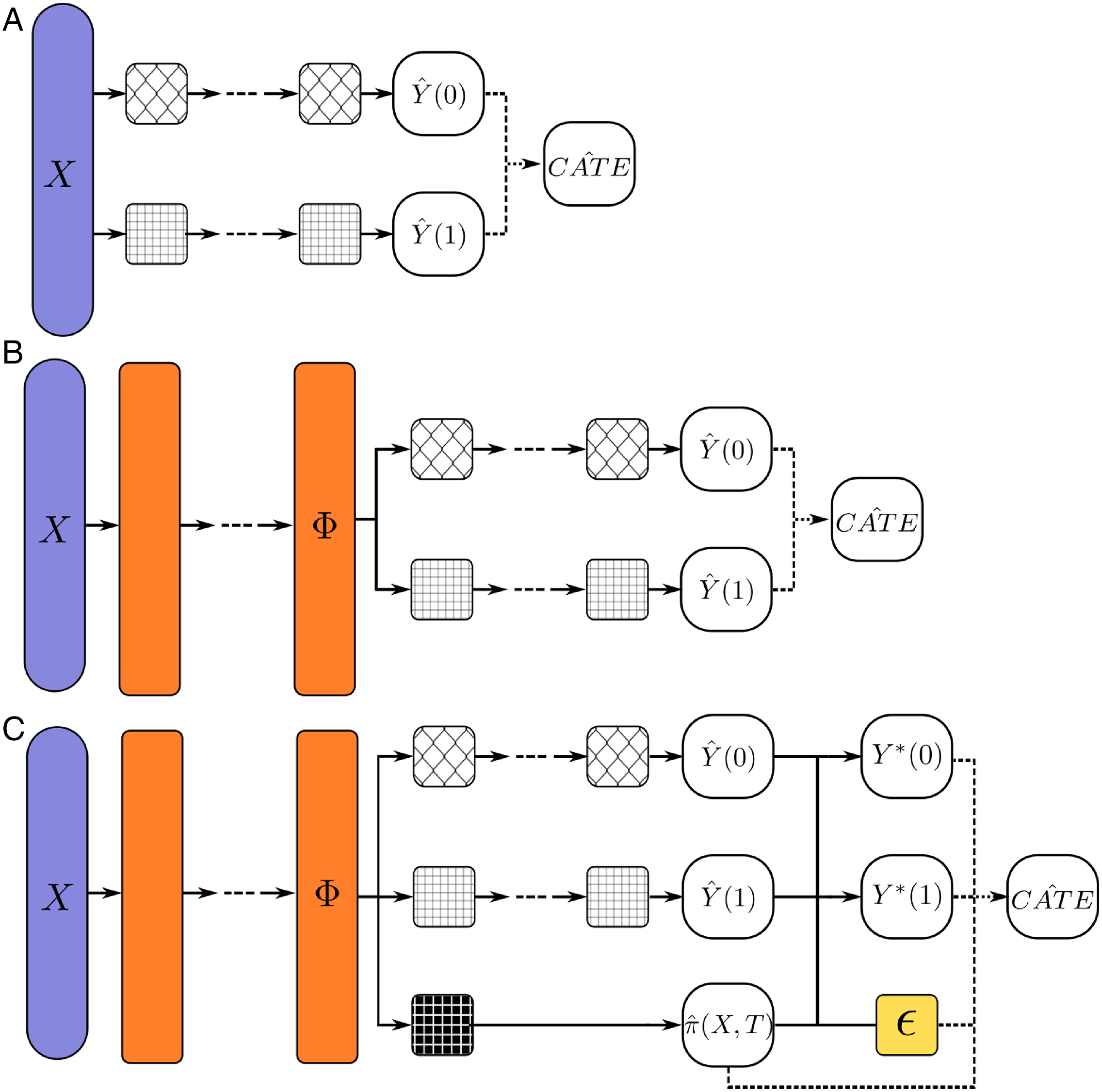
(A) T-learner. In a T-learner, separate feed-forward networks are used to model each outcome (rounded white boxes). We denote the function encoded by these outcome modelers $h$ . (B) TARNet. TARNet extends the T-learner with shared representation layers (orange). The motivation behind TARNet (and further elaborations of this model) is that the multitask objective of accurately predicting both the treated and control potential outcomes forces the representation layers to learn a balancing function $Φ$ such that the $Φ (X | T = 0)$ and $Φ (X | T = 1)$ are overlapping distributions in representation space. For a code implementation, see Box 7. (C) Dragonnet Dragonnet also adds a propensity score head to TARNet (black textured box) and a free “nudge” parameter $ϵ$ . In an adaptation of Targeted Maximum Likelihood Estimation, $\hat{π}$ and $ϵ$ are used to re-weight the outcomes to provide lower biased estimates of the $A T E$ .

After training, inputting the same unit into both networks of a T-learner will produce predictions for both potential outcomes: $\hat{Y} (T)$ and $\hat{Y} (1 - T)$ . We can plug-in these predictions to estimate the $C A T E$ for each unit,

\hat{τ_{i}} = (1 - 2 T_{i}) (\hat{Y_{i}} (1 - T_{i}) - \hat{Y_{i}} (T_{i}))

where the first term is a switch to make sure the treated potential outcome comes first. The ATE can be estimated as,

\hat{A T E} = \frac{1}{N} \sum_{i = 1}^{N} \hat{τ_{i}}

Nearly all of the models described below combine this plug-in outcome modeling approach with other forms of treatment adjustment.

Balancing through Representation Learning

TARNet (Tutorial 1 )

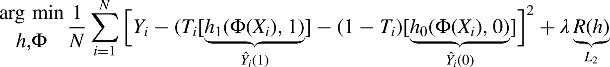
Balancing is a treatment adjustment strategy that aims to deconfound treatment from the outcome by forcing the treated and control covariate distributions closer together (Johansson, Shalit, and Sontag, 2016). The novel contribution of deep learning to the selection of observables literature is the proposal that a neural network can transform the covariates into a representation space $Φ$ such that the treated and control covariate distributions are indistinguishable (Figure 3).

To encourage a neural network to learn balanced representations, the seminal paper in this literature, Shalit, Johansson, and Sontag (2017), proposes a simple two-headed neural network called TARNet that extends the outcome modeling T-learner with shared representation layers (Figure 5B). Each head models a separate potential outcome: one head learns the function $\hat{Y} (1) = h_{1} (Φ (X), 1)$ , and the other head learns the function $\hat{Y} (0) = h_{0} (Φ (X), 0)$ . During training, only one head will receive error gradients at a time (the one predicting the observed outcome). However, both heads backpropagate their gradients to shared representation layers that learn $Φ (X)$ . The idea is that these representation layers must learn to balance the data because they are tasked with predicting both outcomes. The authors of this algorithm have subsequently extended TARNet with additional losses in an algorithm called CFRNET that explicitly encourages balancing by minimizing a statistical distance between the two covariate distributions in representation space; see Online Appendix for details (Johansson et al., 2018, 2020).

The complete objective for the network is to fit the parameters of $h$ and $Φ$ for all $n$ units in the training sample such that,

\begin{matrix} \arg min \\ h, Φ \end{matrix} \frac{1}{N} \sum_{i = 1}^{N} [Y_{i} - (T_{i} [\underset{\hat{Y_{i}} (1)}{\underset{⏟}{h_{1} (Φ (X_{i}), 1)}}] - (1 - T_{i}) [\underset{\hat{Y_{i}} (0)}{\underset{⏟}{h_{0} (Φ (X_{i}), 0)}}]]^{2} + λ \underset{L_{2}}{\underset{⏟}{R (h)}}

(4)

or more compactly,

\binom{\arg \min}{h, Φ} M S E (Y_{i}, \underset{\hat{Y_{i}} (T_{i})}{\underset{⏟}{h (Φ (X_{i}), T_{i})}}) + λ \underset{L_{2}}{\underset{⏟}{R (h)}}

(5)

where

R (h)

is a model complexity term (e.g., for

L_{2}

regularization) and

λ

is a hyperparameter chosen through model selection. For coded versions of TARNet in TensorFlow and Pytorch, see Box 7.

Box 7:

TARNet in Code

Below we show simple implementations of TARNet in Python TensorFlow 2 and Pytorch. For more explanation on this implementation and to run this code on the IHDP data, see the tutorials.

TensorFlow 2 Functional API (Keras)

def make_tarnet(input_dim):

#The argument is the number of X covariates.

x = Input(shape=(input_dim,), name='input')

#In TF fxnl API, stack layers by feeding output of prev layer to next

#Make 2 representation layers

#units is the output dim of layer

#elu is \"xponentiated linear unit" activation fxn

phi = Dense(units=200, activation='elu')(x)

phi = Dense(units=200, activation='elu')(phi)

#Begin separate outcome modeling heads

y0_hidden = Dense(units=100, activation='elu')(phi)

y1_hidden = Dense(units=100, activation='elu')(phi)

#Add second layers

y0_hidden = Dense(units=100, activation='elu'(y0_hidden)

y1_hidden = Dense(units=100, activation='elu')(y1_hidden)

#Output predictions

y0_pred = Dense(units=1, activation=None)(y0_hidden)

y1_pred = Dense(units=1, activation=None)(y1_hidden)

#Bundle outputs

concat_pred = Concatenate(1)([y0_pred, y1_pred])

#instantiate model

model = Model(inputs=x, outputs=concat_pred)

return model

Pytorch

class TARNet(nn.Module):

def __init__(self,input_dim):

super(TARNet,self).__init__()

self.phi = nn.Sequential(

#both input and output dims are specified in torch

nn.Linear(input_dim, 200),

nn.ELU(), #activations are discrete from layers

nn.Linear(200,200),

nn.ELU())

self.y0_hidden = nn.Sequential(

nn.Linear(200, 100),

nn.ELU(),

nn.Linear(100,100),

nn.ELU())

self.y1_hidden = nn.Sequential(

nn.Linear(200, 100),

nn.ELU(),

nn.Linear(100,100),

nn.ELU())

self.y0_pred =nn.Linear(100,1)

self.y1_pred = nn.Linear(100,1)

#the flow of data/gradients in torch is declared in a forward fxn

def forward(self,X):

rep = self.phi(X)

y0_rep=self.y0_hidden(rep)

y0_hat=rep=self.y0_pred(y0_rep)

y1_rep=rep=self.y1_hidden(rep)

y1_hat=rep=self.y1_pred(y1_rep)

return y0_hat, y1_hat

Double Robustness with IPW

Rather than applying losses directly to the representation function, IPW methods estimate propensity scores from representations using the function $π (Φ (X), T) = P (T | Φ (X))$ . As in traditional IPW estimators, these methods exploit the sufficiency of correctly specified propensity scores to reweight the plugged-in outcome predictions and provide unbiased estimates of the ATE (Rosenbaum and Rubin, 1983). Because these models combine outcome modeling with IPW, they retain the attractive statistical properties of doubly robust estimators discussed in the “Treatment Modeling: Nonparametric Matching” section (Atan, Jordon, and Schaar, 2018). In this section, we focus on Shi, Blei, and Veitch (2019)’s Dragonnet model, which adapts semiparametric estimation theory for batch-wise neural network training in a procedure they call “Targeted Regularization” (TarReg) (Kennedy, 2016). Given the increasing importance of semiparametric theory and “double machine learning” across the causal estimation literature, we include a brief introduction to semiparametric theory and targeted maximum likelihood estimation (TMLE) before diving into the details of the Dragonnet algorithm (Van der Laan and Rose, 2011; Chernozhukov et al., 2018).

Dragonnet (Tutorial 3 / Tutorial 4 )

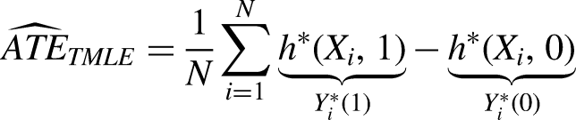
A trivial extension to TARNet is to add a third head to predict the propensity score. This third head could use multiple neural network layers or just a single neuron, as proposed in Dragonnet (Figure 5C) (Shi, Blei, and Veitch, 2019). Dragonnet uses this additional head to develop a training procedure called Targeted Regularization for semiparametric causal estimation, inspired by TMLE (Van der Laan and Rose, 2011).

With three heads, the basic loss function for this network looks like:

\begin{matrix} \arg min \\ h, Φ, π, h \end{matrix} \underset{Outcome \,\,Loss}{\underset{⏟}{M S E (Y_{i}, h (Φ (X_{i}), T_{i})}} + α \underset{π \, L o s s}{\underset{⏟}{BCE (T_{i}, π (Φ (X_{i}), T_{i}))}} + λ \underset{L_{2}}{\underset{⏟}{R (h)}}

(6)

with

α

being a hyperparameter to balance the two objectives, and

λ

balancing these against a model complexity term. The mean squared error and binary cross-entropy are standard objective functions in ML for regression and binary classification, respectively. Note that the first term is the same as the first term in Equation 5.

Below, we explore how the authors add a second loss on top of this one to allow for semiparametric estimation.

Semiparametric Theory of Causal Inference

In recent years, semiparametric theory has emerged as a dominant theoretical framework for applying ML algorithms, including neural networks, to causal estimation (Chernozhukov et al., 2018, 2021, 2022; Farrell, Liang, and Misra, 2021; Kennedy, 2016; Nie and Wager, 2021; Van der Laan and Rose, 2011; Wager and Athey, 2018). The great appeal of these frameworks is that they allow for ML algorithms to be plugged-in for nonlinear estimates of outcomes and propensity score, while still providing attractive statistical guarantees (e.g., consistency, efficiency, asymptotically valid confidence intervals).

At a very intuitive level, semiparametric causal estimation is focused on estimating a target parameter $T (P)$ of a distribution $P$ of treatment effects, i.e., estimating the $A T E$ (Fisher and Kennedy, 2021). While we do not know the true distribution of treatment effects because we lack counterfactuals, we do know some parameters of this distribution (e.g., the treatment assignment mechanism). We can encode these constraints in the form of a likelihood that parametrically defines a set of possible approximate distributions $P$ from our existing data. Within this set, there is a sample-inferred distribution $\tilde{P} \in P$ , that can be used to estimate $T (P)$ using $T (\tilde{P})$ .

Regardless of $\tilde{P}$ chosen, $\tilde{P} \neq P \to T (\tilde{P}) \neq T (P)$ . We do not know how to pick $\tilde{P}$ with finite data to get the best estimate $T (\tilde{P})$ . We can maximize a likelihood function to pick $\tilde{P}$ , but there may be “nuisance” parameters in the likelihood that are not the target and we do not care about estimating accurately. Maximum likelihood optimization may provide lower-biased estimates of these nuisance terms at the cost of better estimates of $T (P)$ .

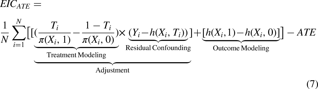
To sharpen the likelihood’s focus on $T (P)$ , we define a “nudge” parameter $ϵ$ that, starting from $\tilde{P}$ , selects a $T ({\tilde{P}}_{ϵ}) \in P$ that is closer to $P$ $T (\tilde{P})$ $T (P)$ . An influence curve of $T (P)$ tells us how changes in $ϵ$ will induce changes in $T ({\tilde{P}}_{ϵ})$ . We’ll use this influence curve to fit $ϵ$ to get a better approximation of $T (P)$ within the likelihood framework. In particular, there is a specific efficient influence curve (EIC) that provides us with the lowest variance estimates of $T (P)$ . In causal estimation, solving the EIC for the ATE yields estimates that are asymptotically unbiased, efficient, and have confidence intervals with (asymptotically) correct coverage.

The EIC for the ATE is,

\begin{aligned} E I C_{A T E} = \\ \frac{1}{N} \sum_{i = 1}^{N} [[\underset{Adjustment}{\underset{⏟}{\underset{Treatment \,Modeling}{\underset{⏟}{(\frac{T_{i}}{π (X_{i}, 1)} - \frac{1 - T_{i}}{π (X_{i}, 0)})}} \times \underset{Residual \,Confounding}{\underset{⏟}{(Y_{i} - h (X_{i}, T_{i}))}}}}] + \underset{Outcome \,Modeling}{\underset{⏟}{[h (X_{i}, 1) - h (X_{i}, 0)]}}] - A T E \end{aligned}

(7)

Setting

E I C_{A T E}

to its mean of 0,

A T E = \frac{1}{N} \sum_{i = 1}^{N} [[\underset{Adjustment}{\underset{⏟}{\underset{Treatment \,Modeling}{\underset{⏟}{(\frac{T_{i}}{π (X_{i}, 1)} - \frac{1 - T_{i}}{π (X_{i}, 0)})}} \times \underset{Residual \,Confounding}{\underset{⏟}{(Y_{i} - h (X_{i}, T))}}}}] + \underset{Outcome \,Modeling}{\underset{⏟}{[h (X_{i}, 1) - h (X_{i}, 0)]}}]

(8)

The underbraces illustrate how

E I C_{A T E}

resembles a doubly robust estimator. When the EIC is minimized (set to 0) as in Equation 8, the

A T E

is equal to the outcome modeling estimate plus a treatment modeling estimate proportional to the residual error.

From TMLE to Targeted Regularization

Targeted Regularization (TarReg) is closely modeled after Targeted Maximum Likelihood Estimation (TMLE) (Van der Laan and Rose, 2011). TMLE is an iterative procedure where a nuisance parameter $ϵ$ is used to nudge the outcome models towards sharper estimates of the ATE when minimizing the EIC as in Equation 8.¹¹

Fit $h$ by predicting outcomes (e.g., using TARNet) and minimizing $M S E (Y_{i}, h (Φ (X_{i}), T_{i}))$

Fit $π$ by predicting treatment (e.g., using logistic regression) and $B C E (T_{i}, π (Φ (X_{i}), T_{i}))$

Plug-in $h$ and $π$ functions to fit $ϵ$ and estimate $h^{*} (X, T)$ where,

\underset{Y *}{\underset{⏟}{h^{*} (X_{i}, T_{i})}} = \underset{\hat{Y}}{\underset{⏟}{h (Φ (X_{i}), Φ (T_{i}))}} + \underset{Treatment\ Modeling\ Adjustment}{\underset{⏟}{(\frac{T_{i}}{π (Φ (X_{i}), 1)} - \frac{1 - T_{i}}{π (Φ (X_{i}), 0)})}} \times \underset{“ nudge ”}{\underset{⏟}{ϵ}}

by minimizing

M S E (Y, h^{*} (Φ (X), T))

. This is equivalent to minimizing the “Adjustment” part in Equation 8.

Plug-in $h * (X, T)$ to estimate $\hat{A T E}$ :

{\hat{A T E}}_{T M L E} = \frac{1}{N} \sum_{i = 1}^{N} \underset{Y_{i} * (1)}{\underset{⏟}{h * (X_{i}, 1)}} - \underset{Y_{i} * (0)}{\underset{⏟}{h * (X_{i}, 0)}}

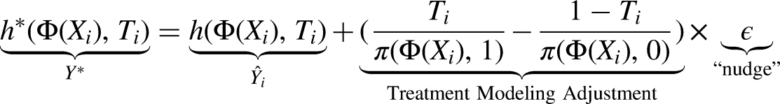
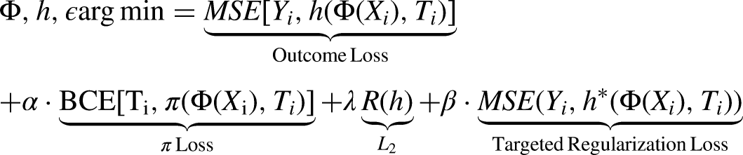
Targeted Regularization takes TMLE and adapts it for a neural network loss function. The main difference is that steps 1 and 2 above are done concurrently by Dragonnet, and that the loss functions for the first three steps are combined into a single loss applied to the whole network at the end of each batch. It requires adding a single free parameter to the Dragonnet network for

ϵ

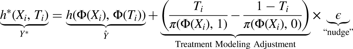
At a very intuitive level, Targeted Regularization is appealing because it introduces a loss function to TARNet that explicitly encourages the network to learn the mean of the treatment effect distribution, and not just the outcome distribution. The Targeted Regularization procedure proceeds as follows:

In each epoch:

Use Dragonnet to predict $h (Φ (X), T)$ and $π (Φ (X), T)$ .

Calculate the standard ML loss for the network using a hyperparameter $α$ :

\begin{matrix} \arg min \\ h, Φ, π, h \end{matrix} \underset{Outcome\ Loss}{\underset{⏟}{M S E (Y_{i}, h (Φ (X_{i}), T_{i}))}} + α \underset{π \ Loss}{\underset{⏟}{BCE (T_{i}, π (Φ (X_{i}), T_{i}))}} + λ \underset{L_{2}}{\underset{⏟}{R (h)}}

Compute $h^{*} (Φ (X_{i}), T_{i})$ as above,

\underset{Y *}{\underset{⏟}{h^{*} (Φ (X_{i}), T_{i})}} = \underset{\hat{Y_{i}}}{\underset{⏟}{h (Φ (X_{i}), T_{i})}} + \underset{Treatment\ Modeling\ Adjustment}{\underset{⏟}{(\frac{T_{i}}{π (Φ (X_{i}), 1)} - \frac{1 - T_{i}}{π (Φ (X_{i}), 0)})}} \times \underset{“ nudge ”}{\underset{⏟}{ϵ}}

Calculate the targeted regularization loss: $M S E (Y, h * (Φ (X), T))$

Combine and minimize the losses from 1 and 2 using a hyperparameter $β$ ,

{\begin{aligned} \underset{Φ, h, ϵ}{\arg min} = \underset{Outcome \,Loss}{\underset{⏟}{M S E [Y_{i}, h (Φ (X_{i}), T_{i})]}} \\ + α \cdot \underset{π \,Loss}{\underset{⏟}{BCE [T_{i}, π (Φ (X_{i}), T_{i})]}} + λ \underset{⏟}{R (h)} \end{aligned}}_{L_{2}} + β \cdot \underset{Targeted \,Regularization\, Loss}{\underset{⏟}{M S E (Y_{i}, h^{*} (Φ (X_{i}), T_{i}))}}

Step 3 of Targeted Regularization is exactly equivalent to minimizing the EIC up to a constant

β

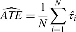
At the end of training, we can thus estimate the targeted regularization estimate of the ATE $\hat{A T E_{T R}}$ as in TMLE:

\hat{A T E_{T R}} = \frac{1}{N} \sum_{i = 1}^{N} \underset{Y *_{i} (1)}{\underset{⏟}{h * (Φ (X_{i}), 1)}} - \underset{Y *_{i} (0)}{\underset{⏟}{h * (Φ (X_{i}), 0)}}

Compared to S-learners, T-learners, and TARNet, the Dragonnet algorithm is particularly attractive because of the statistical guarantees afforded by its semiparametric framework. It is doubly robust, unbiased, converges at a rate of

\frac{1}{\sqrt{n}}

, and the sampling distribution is asymptotically normal. Below we describe how to create assymptotically valid confidence intervals for this estimator.

Confidence and Interpretation

In this section, we move from theory to practice and treat best practices for building confidence intervals and interpreting heterogeneous treatment effects. Both of these topics are active areas of development, not only within the causal inference literature but across ML research. Here we specifically focus on recommendations that can be easily implemented by analysts.

Assessing Confidence

(Tutorial 4 )

In this paper, we feature Dragonnet over other approaches because of its attractive statistical properties. Because the Targeted Regularization procedure in Dragonnet is essentially a variant of TMLE, an asymptotically valid standard error can be calculated as the sample corrected variance of the EIC $σ_{\hat{A T E}}$ , where

σ_{\hat{A T E_{T R}}} = \sqrt{\frac{V a r (E I C_{\hat{A T E_{T R}}})}{N}}

(9)

and,

V a r (E I C_{\hat{A T E_{T R}}}) = V a r [(\frac{T_{i}}{π (X_{i}, 1)} - \frac{1 - T_{i}}{π (X_{i}, 0)}) (Y - h * (X_{i}, T_{i})) + (h * (X_{i}, 1) - h * (X_{i}, 0)) - \hat{A T E_{T R}}]

(10)

(Van der Laan and Rose, 2011, pp. 96)

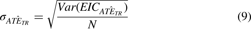
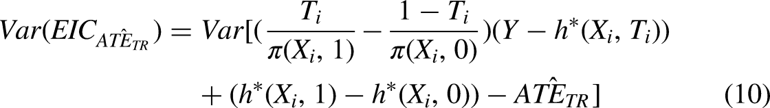
In Tutorial 4, we show how $σ_{\hat{A T E}}$ can be used to calculate a Wald confidence interval for Dragonnet. While not featured in this review, asymptotically valid conference intervals can also be calculated using RieszNet, a variant of Dragonnet introduced in Chernozhukov et al. (2022) that connects neural network estimation to the automatically debiased ML literature currently popular in causal econometrics (Chernozhukov et al., 2018, 2021).

Interpretation

(Tutorial 4 )

A lack of interpretability has been a barrier to the adoption of ML methods like neural networks and random forests in social science settings. However, the literature on post hoc interpretability techniques has matured considerably over the past five years, and several techniques for identifying important features/covariates such as permutation importance, LIME scores, SHapley Additive exPlanations (SHAP) scores, Individual Conditional Expectation plots etc. are in widespread usage today (Altmann et al., 2010; Goldstein et al., 2015; Lundberg and Lee, 2017; Ribeiro, Singh, and Guestrin, 2016). For a broad and accessible treatment of interpreting ML models see Molnar (2022).

Building on criteria used to evaluate other explainable AI methods, Crabbé et al. (2022) note four desirable properties of a feature importance technique for the interpretation of deep causal estimators: Sensitivity, completeness, linearity, and implementation invariance (Sundararajan, Taly, and Yan, 2017). A method that is sensitive can distinguish between features that are simply predictive of the outcome, and those that actually influence CATE heterogeneity. A method that is complete identifies all features that, together, explain all effect heterogeneity compared to a baseline. A linear method is one where the feature importance scores additively describe the prediction. Lastly, the approach should be agnostic to both the model architecture (e.g., TARNet, Dragonnet) and different architectural hyperparameterizations (i.e., invariant to implementation). Of the feature importance methods surveyed, they identify two that manifest all four of these qualities: SHAP scores, and integrated gradients.

SHAP scores have emerged as one of the most popular methods for evaluating ML models in recent years (Lundberg and Lee, 2017). SHAP is what is called a “local” interpretability method: it provides feature importance estimates for each individual datum. Theoretically, SHAP frames feature importance estimation as a cooperative (game-theoretic) game between covariates to predict a specific outcome. Under the hood, the algorithm exhaustively compares all possible “coalitions” of covariates and their ability to predict the outcome (win the game). Predictions from this powerset of coalitions are used to calculate the additive marginal contributions of each feature in prediction using Shapley values. The disadvantage of SHAP is that, even with computational tricks, calculating scores for every unit can become computationally intractable in high-dimensional datasets. SHAP scores are interpreted in comparison to a causal baseline of the ATE.

Because of the computational expense of SHAP scores, Crabbé et al. (2022) also recommend another local-interpretability method called “Integrated Gradients” (Sundararajan, Taly, and Yan, 2017). Intuitively, this algorithm draws a straight-line, linear path in feature space between the target input (individual unit) and a baseline (i.e., a hypothetical unit who is exactly average on all covariates). A feature importance score can then be constructed by calculating the gradient in prediction error along this path with respect to the feature of interest. Note that SHAP scores can also be understood theoretically within the path framework. From this perspective, coalitions are paths in which each feature is turned on sequentially, and the SHAP score is the expectation across these paths. This interpretation leads to a gradient-based algorithm for calculating SHAP scores specifically for neural networks, which is also in the SHAP package. In practice, we recommend that analysts experiment with both integrated gradients and SHAP scores.

What’s in the tutorials?

To move from theory to empirics, the online tutorials show how to implement many of the ideas presented throughout this primer. The tutorials are hosted in notebooks in the Google Colaboratory environment. When users open a Colab notebook, Google immediately provides a free virtual machine with standard Python ML packages available. This means that readers need not install anything on their own computers to experiment with these models. The tutorials are written in the Python programming language and provide examples in both TensorFlow2 and Pytorch, the two most popular deep learning frameworks. We note that both TensorFlow2 and Pytorch have implementations in R. However, we strongly recommend that readers interested in getting into deep learning work in Python, which has a much richer ecosystem of third-party packages for ML.

Currently there are five tutorials:

Tutorial 1 introduces S-learners, and T-learners before TARNet as a way to get familiar with building custom TensorFlow models.

Tutorial 2 focuses on causal inference metrics and hyperparameter optimization. Because we do not observe counterfactual outcomes, it’s not obvious how to optimize supervised learning models for causal inference. This tutorial introduces some metrics for evaluating model performance. In the first part, you learn how to assess performance on these metrics in Tensorboard. In the second part, we hack Keras Tuner to do hyperparameter optimization for TARNet, and discuss considerations for training models as estimators rather than predictors.

Tutorial 3 highlights the semiparametric extension to TARNet featured in Shi, Blei, and Veitch (2019). We add treatment modeling to our TARNet model, and build an augmented inverse propensity score estimator. We then briefly describe the algorithm for Targeted Maximum Likelihood Estimation to introduce and build a Dragonnet with Shi et al.’s Targeted Regularization.

Tutorial 4 reimplements Dragonnet in Pytorch and shows how to calculate asymptotically valid confidence intervals for the ATE. We also interpret the features contributing to different heterogeneous CATEs using Integrated Gradients and SHAP scores. This tutorial is a good tutorial if you also just want to learn how to interpret SHAP scores, independent of the context of causal inference.

Tutorial 5 features the Counterfactual Regression Network (CFRNet) and propensity-weighted CFRNet in Shalit, Johansson, and Sontag (2017); Johansson et al. (2018, 2020) (see Online Appendix). This approach relies on integral probability metrics to bind the counterfactual prediction loss and force the treated and control distributions closer together. The weighted variant adds adaptive propensity-based weights that provide a consistency guarantee, relax overlap assumptions, and ideally reduce bias.

Beyond Traditional Data: Text, Networks, Images, and Treatment over Time

As exciting as neural networks are for heterogeneous treatment effect estimation from quantitative data, a great promise of deep causal estimation is inference when treatments, confounders, and mediators are encoded in high-dimensional data (e.g., text, images, social networks, speech, and video) or are time-varying. This is a strong advantage of neural networks over other ML approaches, which do not generalize competitively to nonquantitative data. In these scenarios, multitask objectives and tailored architectures can be used to learn representations that are simultaneously rich, capture information about causal quantities, and disentangle their relationships. Moreover, the inherent flexibility of neural networks means that, in many cases, the TARNet-style models presented above can serve as the foundations to inference on text and graphs with some architectural modifications, additional losses, and new identification assumptions.

This literature is rapidly evolving, so readers should treat this section of the primer as fundamentally prospective. To maintain accessibility, our primary goal here is to introduce readers to hypothetical scenarios where they might perform causal inference on text, network, or image data. Second, we selectively review contemporary, theoretically motivated literature on deep causal estimation in these settings. The identification assumptions for different data types differ substantially, so we generally leave those to the interested reader. Finally, we briefly discuss approaches for dealing with time-varying confounding. We also take this section as an opportunity to introduce Graph Neural Networks (GNNs) and the Transformer architecture, now used in most contemporary deep learning models to learn from complex data (Box 8). Box 8:

Graph Neural Networks and Transformers

Graph neural networks (GNNs) are the current state-of-the-art approach for creating representations for nodes in graphs. Compared to previous approaches that relied on “shallow” embeddings based only on a node’s local context (e.g., random walks to nearby nodes), GNNs are attractive because their node representations are aggregated from the structural position and covariates of all nodes $n$ degrees away from the target node, where $n$ is the number of graph neural network layers.

The most intuitive understanding of how graph neural networks work is as a message-passing system (Gilmer et al., 2017). We use one of the first GNN papers, the Graph Convolutional Network as an example (Kipf and Welling, 2017). In this interpretation, each node has a message that it passes to its neighbors through a graph convolution operation. In the first layer of a GNN this message would consist of the node’s covariates/features. In consecutive layers of the network, these messages are actually representations of the node produced by the previous layer. During graph convolution, each node multiplies incoming messages by its own set of weights and combines these weighted inputs using an aggregation function (e.g., summation). By the $n$ -th GNN layer, these messages will contain structure and covariate information from all nodes $n$ degrees away. For interested readers, there is also a spectral interpretation of this process. Typically GNNs are trained to produce representations of graphs by predicting the probability that two nodes are linked in the network, and then used for something else. One variant of the GNN uses an “attention” mechanism to vary the extent that nodes value messages from different neighbors (the graph attention network or GAT) (Veličković et al., 2018).

As of 2023, Transformers are the hegemonic architecture used in natural language processing. After their introduction in 2017, these models improved performance on many high-profile NLP tasks across the board. Several enterprise-scale transformers have been featured in the media for their impressive performance in text generation and question answering (e.g. OpenAI’s GPT-3/4, Google’s Bard, Meta’s Llamma). Smaller models in broad use are based on the BERT architecture (Devlin et al., 2019).

Transformers and GNNs, specifically GATs, are roughly equivalent architectures. From the graph perspective, words in sentences are akin to nodes in networks, with their relative positions to each other being analogous to their structural positions in the graph. Transformers improved on previous sequential approaches to text analysis (i.e. recurrent neural networks) by having each word (or representation of a word) receive messages from not just adjacent words, but all words heterogeneously. Attention mechanisms throughout the architecture allow each layer of a transformer to attend to words or aggregated representation heterogeneously. Architectures such as BERT or GPT stack transformer layers to create models with hundreds of millions to hundreds of billions of parameters. These models are expensive to train, both computationally and with respect to data, so they are often pretrained on enormous datasets and then “fine-tuned” (lightly re-trained) with smaller datasets for specific tasks or to align with certain goals.

Causal Inference from Text

In recent years, an interdisciplinary community across both social science and computer science has coalesced around causal inference from text (see Keith, Jensen, and O’Connor (2020) and Feder et al. (2021) for exhaustive reviews). Broadly speaking, texts may capture information about any causal quantity (treatments, outcomes, confounders, mediators) we might be interested in. For example, in an exit-polling experiment, analysts might want to measure toxicity ( $Y$ ) in text responses to political prompts. In an observational study of e-mail response times ( $Y$ ), analysts might want to measure the effects of the tone of the email ( $T$ ). In this scenario, the analyst might also want to control for confounders like subject matter ( $X$ ). Each of these scenarios presents distinct identification challenges (Feder et al., 2021). But in all cases, we can use low-dimensional representations of the high dimensional text to extract, quantify, and disentangle relationships between nuanced qualities like tone and subject matter.

The ability of neural networks to automatically extract features makes them particularly suited for the last scenario when both treatment information and confounding covariates are encoded in text. In many cases, we may not have explicitly identified, quantified, or labeled all of the confounders in text (e.g., subject matter and tone of emails), but we would still like to control for them. Pryzant et al. (2021),Veitch, Sridhar, and Blei (2020), and Gui and Veitch (2022) address this problem by prepending Transformer-layers (Box 8) for reading text to the beginning of TARNet or Dragonnet. Veitch, Sridhar, and Blei (2020) demonstrate the viability of this approach on a Science of Science question testing the causal effect of equations on getting papers accepted to computer science conferences. Pryzant et al. (2021); Gui and Veitch (2022) explore the more complicated scenario in which the treatment is not explicitly known (e.g., equations in papers, gender of authors), but is instead externally perceived upon reading (e.g., politeness/rudeness of an email or toxicity of a social media post). In these models, an additional loss function is also added for learning text representations concurrently with the causal inference losses discussed above.

Causal Inference from Networks

A smaller literature has leveraged relational data for causal inference in two distinct scenarios. In the first traditional selection on the observable setting, we wish to control for information about unobserved confounding inferable from homophilous ties. For example, age or gender might be unmeasured in our data, but we might expect people to develop friendship ties with those of the same gender identity or age cohort.

This scenario suggests estimation strategies similar to those when confounders are encoded in text. Much like Transformer layers can be prepended to TARNet-style estimators to learn from text, GNNs (an analog of the Transformer) can be preprended to learn from graphs. Guo, Li, and Liu (2020) provides a first pass at this problem by adding GNN layers to CFRNet Shalit, Johansson, and Sontag (2017) (Box 8). Veitch, Wang, and Blei (2019) instead adapt Dragonnet in a semiparametric framework to allow for consistent estimates of the treatment and outcome, assuming the network representation encodes significant information about confounders.

The second, more challenging scenario is estimating the causal effect of social influence on outcomes from observational data. For example, Cristali and Veitch (2022) introduce the problem of measuring the effects of vaccination ( $T$ ) on peer vaccination choice ( $Y$ ). This is a hard problem because (a) SUTVA is a fundamental assumption of all causal inference frameworks and (b) it is hard to disentangle whether changes in the outcome result from the treatment via peer effects (e.g, person A pressuring person B to vaccinate), or from homophily (e.g., person A and person B having similar political leanings). In other words, contagion and homophily are generically confounded (Shalizi and Thomas, 2011). McFowland and Shalizi (2023) are the first to tackle this problem by making strong parametric assumptions about the generation of network ties and the outcome model. Cristali and Veitch (2022) instead propose an approach using neural network-learned representations of the graph.

Causal Inference from Images

While ideas from causal inference have been leveraged extensively to improve image classification, to our knowledge there are no papers that explore causal inference where treatments, confounders, mediators, or predictors are encoded in images.¹² That being said, some scenarios proposed for causal text analysis should apply here as well. For example, consider the conjoint experiment on the electability of politicians’ faces by Todorov et al. (2005) where both the treatment (e.g. incumbency of a politician) and potential latent confounders (e.g., party, age, gender, race) are encoded in an image. In this setting, a TARNet-like model adapted to learn and condition on image representations could improve treatment effect estimation by controlling for confounders such as the politician’s age. Causal inference on images is an area ripe for exploration, and we hope to see more work here in the future.

Causal Inference from Time-varying Data

One natural extension of deep causal estimation is to scenarios where treatments are administered over time and confounding may be time-varying. While “g-methods” developed by Robins et al. for estimating effects with time-varying treatments and confounding have existed for decades, the statistical assumptions encoded in these models are quite strong (Robins, 1994; Robins and Hernán, 2008; Robins, Hernan, and Brumback, 2000). Due to their reliance on generalized linear models to define the “structural” component, they assume that the outcome is a linear function of all covariates and treatment. Second, for identification, they make strong assumptions about which previous timesteps confound the current one. Third, they require different coefficients to be estimated at each time steps. Transformers (Box 8) and RNNs, a simpler model for sequential data (Online Appendix), should be able to capture long-term dependencies and nonlinearities in ways that marginal structural models and g-computation cannot.

Several papers have begun to explore these possibilities in the context of personalized medicine. Lim, Alaa, and van der Schaar (2018) build a marginal structural model using a RNN, and Bica et al. (2020) extend this framework with an additional loss to more explicitly deal with time varying confounding by forcing the model to “unlearn” information about the previous time steps. Melnychuk, Frauen, and Feuerriegel (2022) go one step further by adapting Bica et al. (2020)’s approach with a transformer. Inspired by longitudinal targeted maximum likelihood, Frauen et al. (2022) add a semiparametric targeting layer to their RNN to create a g-computation algorithm that is doubly robust and asymptotically efficient. Li et al. (2021) instead propose an RNN framework for g-computation that allows for dynamic treatment regimes. All of these papers use simulations of tumor growth dynamics, naturalistic simulations based on vital signs from intensive care unit visits, or datasets on the response of back pain to physical therapy.

Conclusion: Deep Causal Estimation in Context

In this primer, we introduce social scientists to the emerging ML literature on deep learning for causal inference. To set the stage, we first provide both an intuitive introduction to fundamental deep learning concepts like representation and multitask learning, as well as practical guidelines for training neural networks. In the main body of the article, we show how ML researchers have adapted core treatment and outcome modeling strategies to leverage the particular strengths of neural networks for heterogeneous treatment effect estimation. We follow with a discussion on inference (e.g., model selection, confidence intervals, interpretation), and close with a prospective look at algorithms for inference from text, social networks, images, and time-varying data.

Deep learning is not the only potential tool for heterogeneous treatment effect inference, and there are robust literatures exploring the usage of other methods in both the econometrics and biostatistics communities (Van der Laan and Rose, 2011; Chernozhukov et al., 2018; Wager and Athey, 2018). While these literatures are certainly more mature, below we discuss reasons why we think the use gap between neural networks and other ML methods will continue to narrow, a change that we must prepare for.

First, neural networks are better at modeling nonlinear heterogeneity (e.g., in treatment responses) than other ML methods. In extensive simulations, Curth et al. (2021) found that when the data-generating process for treatment heterogeneity includes exponential relationships, neural networks outperformed random forests, but tree-based methods are robust when the data-generating process is built on linear functions. Neural networks were also consistently better at predicting outlier treatment effects than forests. These differences result from how the two methods model functions. While neural networks can approximate any continuous function with enough neurons, random forests must build nonlinear or nonorthogonal decision boundaries using piecewise functions and average predictions. Consistent with these differences, Curth et al. (2021) also find that neural networks do better when variables are constructed as continuous covariates, and vice versa when they are dichotomized.

From a statistical perspective, the rise of semiparametric and double ML frameworks has also narrowed the gap between neural networks and other types of ML in terms of theoretical guarantees. For example, the TMLE-inspired Dragonnet algorithm featured here is unbiased, plausibly consistent, and converges to the target estimand at a fast rate of $\frac{1}{\sqrt{n}}$ . The closely related Riezsnet double ML model (not featured) boasts similar guarantees (Chernozhukov et al., 2022). Beyond these algorithms, there is a growing adjacent literature of model-agnostic plug-in learners (e.g., X-learner, R-learner) that can leverage the strengths of neural networks (Nie and Wager, 2021; Künzel et al., 2019).

Third, folk beliefs about the data-hungriness and uninterpretability of neural networks are overstated. Neural networks are data-hungry when over-parameterized or learning from high-dimensional data like images, but we show in the tutorials that modest-sized (hundreds of neurons), well-regularized neural networks can successfully infer heterogeneous treatment effects in a naturalistic simulation of quantitative data with less than 800 units. In the “Confidence and Interpretation” section, we also highlight the considerable progress in ML interpretability over the past five years, much of which has been on model-agnostic approaches that benefit all black-box algorithms equally.¹³

In our opinion, the most pressing limitation of current deep learning approaches is the difficulty of optimizing neural networks. Theoretically, this stems from (a) the complexity of the loss functions which are often nonconvex, and (b) the ease of over-parameterizing these models to fit these functions. If neural networks are to be used as statistical estimators, statistical guarantees must be backed by optimization guarantees and/or more rigorous methods for model selection. Outside of statistical estimation, this limitation has largely been addressed through empirical testing on test data and strategic model selection. Within the statistical estimation context, this gap will likely need to be addressed by simulation-based sensitivity analyses and, in the short term, comparisons to other model families.

Moreover, there has been a lack of mature tools and empirical applications of these models. A major goal of this primer, and the tutorials in particular, is to synthesize the theoretical literature, practical training and interpretation guidelines, and annotated code in one place so that social scientists can start using these models. Deep learning frameworks like TensorFlow and Pytorch are becoming more accessible every year, but we note that canned Python packages like Uber’s causalML exist for interested readers who just want to experiment with a few of these models (Chen et al., 2020).

Despite current limitations, we believe the future of causal estimation runs through deep learning. As causal inference ventures into new settings, the flexibility of neural networks will become essential for learning from text, graph, image, video, and speech data. For time-varying settings, we believe the ability of neural networks to model nonlinearities and long-range temporal dependencies will ultimately lead to solutions with net weaker assumptions than current approaches. Overall, we are optimistic and excited to see where deep causal estimation heads over the next few years.

Supplemental Material

sj-pdf-1-smr-10.1177_00491241241234866 - Supplemental material for A Primer on Deep Learning for Causal Inference

Supplemental material, sj-pdf-1-smr-10.1177_00491241241234866 for A Primer on Deep Learning for Causal Inference by Bernard J. Koch, Tim Sainburg, Pablo Geraldo Bastías, Song Jiang, Yizhou Sun, and Jacob G. Foster in Sociological Methods & Research

Footnotes

Declaration of Conflicting Interests

The authors declared no potential conflicts of interest with respect to the research, authorship, and/or publication of this article.

Funding

The authors received no financial support for the research, authorship and/or publication of this article.

ORCID iDs

Bernard J. Koch

Jacob G. Foster

Data Availability Statement

The tutorials use the IHDP naturalistic simulation introduced in Hill (2011) as an example. The 25 covariates/features for the 747 units (139 treated) in the dataset were taken from an experiment, but Hill simulated the outcomes to create known counterfactuals. The data are available from Fredrik Johansson’s website .

Supplemental Material

Supplemental material for this article is available online.

Notes

Author Biographies

Bernard J. Koch is a postdoctoral fellow in the Center for Science of Science and Innovation at the Kellogg School of Management, Northwestern University. He is also an incoming assistant professor at the University of Chicago in the Department of Sociology. His research develops and deploys mechanistic models to explain the evolution of scientific and cultural fields. Current questions include how AI became dominated by deep learning, why problematic race science persists in psychology, and how music genres develop. He also has eccentric interests in deep learning, causal inference, networks, and Bayesian modeling. His work has been published at Sociological Methodology, NeurIPS, and WWW, among other venues.

Tim Sainburg is a postdoctoral scholar at Harvard Medical School in the Department of Neurobiology and at Harvard University in the Department of Molecular and Cellular Biology and the Department of Organismal and Evolutionary Biology. He is a cognitive scientist with broad interest relating to intelligent behavior across species. He employs methods in behavioral sciences, computational sciences, and biological sciences to study how and why intelligent organisms behave. His work has appeared in PLoS Computational Biology, Neural Computation, and Nature Communications, among other venues.

Pablo Geraldo Bastías is a postdoctoral prize research fellow at Nuffield College, University of Oxford. He is affiliated with the Leverhulme Centre for Demographic Science (Oxford), and the Practical Causal Inference Lab and Social Inequality Data Science Lab (UCLA). His research focuses on the social determinants and the stratification consequences of intelligence and learning. Methodologically, he is working on developing tools to help researchers to credibly and transparently identify causal relationships in complex social settings. His work has been published in Sociological Methodology, Oxford Bibliographies in Sociology, Nicotine & Tobacco Research, and Research in Social Work Practice, among others.

Song Jiang is a PhD student in the Department of Computer Science at UCLA. Currently, his research focuses on language models, with a focus on improving language models' reasoning capability for complex tasks. He has also worked on geometric machine learning, causal machine learning and dynamical system forecasting. He won the Best Student Paper Award at the ACM Web Conference (WWW) 2023.

Yizhou Sun is an associate professor in the Department of Computer Science at UCLA. Her principal research interest is on mining graphs/networks, and more generally in data mining, machine learning, and network science, with a focus on modeling novel problems and proposing scalable algorithms for large-scale, real-world applications. She is a pioneer in mining heterogeneous information network, with a recent focus on deep learning on graphs and neural symbolic reasoning. She has over 180 publications in books, journals, and major conferences. She is an ACM Distinguished Member and the recipient of multiple Best Paper Awards, the ACM SIGKDD Doctoral Dissertation Award, an NSF CAREER Award, Amazon Research Awards (twice), and many other prestigious awards. She is a general co-chair of SIGKDD 2023 and PC co-chair of ICLR 2024.

Jacob G. Foster is professor of Informatics and Cognitive Science at Indiana University Bloomington, adjunct professor of Sociology at UCLA, and external professor at the Santa Fe Institute. He uses tools from machine learning and complexity science to study the social production of collective intelligence and the structure and dynamics of ideas in a range of contexts, from science, technology, and culture to AI and SETI. His work blends sophisticated computational and mathematical techniques with social theory and philosophy to clarify key ideas and develop new conceptual frameworks. He is co-Director of the Diverse Intelligences Summer Institute, which cultivates the study of intelligences of diverse forms and formats—from ants and apes to humans and AI. His work has appeared in outlets like American Sociological Review, Science, PNAS, NeurIPS, Philosophical Transactions of the Royal Society B, Sociological Methods & Research, Critical Inquiry, and Public Culture. He was recently an Infosys Member in the School of Social Science at the Institute for Advanced Study (2020-2021).

References

Alaa

Ahmed

Van Der Schaar

Mihaela

. 2019. “Validating Causal Inference Models via Influence Functions.” In International Conference on Machine Learning, volume 36, pp. 191–201. Association for Computing Machinery.

Altmann

André

Toloşi

Laura

Sander

Oliver

Lengauer

Thomas

. 2010. “Permutation Importance: a Corrected Feature Importance Measure.” Bioinformatics (Oxford, England) 26: 1340–7.

Atan

Onur

Jordon

James

Van Der Schaar

Mihaela

. 2018. “Deep-Treat: Learning Optimal Personalized Treatments from Observational Data Using Neural Networks.” In Association for the Advancement of Artificial Intelligence Conference on Artificial Intelligence, volume 32, p. 2071–2078. Association for the Advancement of Artificial Intelligence.

Athey

Susan

Imbens

Guido

. 2016. “Recursive Partitioning for Heterogeneous Causal Effects.” Proceedings of the National Academy of Sciences 113: 7353–60.

Austin

Peter C

. 2011. “An Introduction to Propensity Score Methods for Reducing the Effects of Confounding in Observational Studies.” Multivariate Behavioral Research 46: 399–424.

Bengio

Yoshua

. 2013. “Deep Learning of Representations: Looking Forward.” In International Conference on Statistical Language and Speech Processing, pp. 1–37. Association for Computing Machinery.

Benkeser

Carone

Van Der Laan

MJ.

Gilbert

P.B.

. 2017. “Doubly Robust Nonparametric Inference on the Average Treatment Effect.” Biometrika 104: 863–80.

Benkeser

David

Chambaz

Antoine

. 2020. “A Ride in Targeted Learning Territory.” Journal de la société française de statistique 161: 201–86.

Bica

Ioana

Alaa

Ahmed M.

Jordon

James

van der Schaar

Mihaela

. 2020. “Estimating Counterfactual Treatment Outcomes Over Time through Adversarially Balanced Representations.” In International Conference on Learning Representations, volume 37. Association for Computing Machinery.

10.

Brand

Jennie E

Koch

Bernard

Jiahui

. 2020. “Machine Learning.” In Sage Research Methods Foundations. SAGE.

11.

Chen

Huigang

Harinen

Totte

Lee

Jeong-Yoon

Yung

Mike

Zhao

Zhenyu

. 2020. “CausalML: Python Package for Causal Machine Learning.”.

12.

Chernozhukov

Victor

Chetverikov

Denis

Demirer

Mert

Duflo

Esther

Hansen

Christian

Newey

Whitney

Robins

James

. 2018. “Double/debiased Machine Learning for Treatment and Structural Parameters.” The Econometrics Journal 21: C1–C68.

13.

Chernozhukov

Victor

Newey

Whitney K

Quintas-Martinez

Victor

Syrgkanis

Vasilis

. 2021. “Automatic debiased machine learning via neural nets for generalized linear regression.” arXiv preprint arXiv:2104.14737.

14.

Chernozhukov

Victor

Newey

Whitney

Quintas-Martinez

Victor M

Syrgkanis

Vasilis

. 2022. “Riesznet and forestriesz: Automatic debiased machine learning with neural nets and random forests.” In International Conference on Machine Learning, pp. 3901–3914. PMLR.

15.

Crabbé

Jonathan

Curth

Alicia

Bica

Ioana

van der Schaar

Mihaela

. 2022. “Benchmarking heterogeneous treatment effect models through the lens of interpretability.” arXiv preprint arXiv:2206.08363.

16.

Cristali

Irina

Veitch

Victor

. 2022. “Using Embeddings for Causal Estimation of Peer Influence in Social Networks.” ArXiv abs/2205.08033.

17.

Curth

Alicia

Svensson

David

Weatherall

Jim

van der Schaar

Mihaela

. 2021. “Really Doing Great at Estimating CATE? A Critical Look at ML Benchmarking Practices in Treatment Effect Estimation.” In Proceedings of the Neural Information Processing Systems Track on Datasets and Benchmarks, edited by J. Vanschoren and S. Yeung, volume 1.

18.

Cybenko

George

. 1989. “Approximation by Superpositions of a Sigmoidal Function.” Mathematics of Control, Signals and Systems 5: 455.

19.

Devlin

Jacob

Chang

Ming-Wei

Lee

Kenton

Toutanova

Kristina

. 2019. “BERT: Pre-training of Deep Bidirectional Transformers for Language Understanding.” In Conference of the North American Chapter of the Association for Computational Linguistics: Human Language Technologies, pp. 4171–4186. Association for Computational Linguistics.

20.

Farrell

Max H

Liang

Tengyuan

Misra

Sanjog

. 2021. “Deep Neural Networks for Estimation and Inference.” Econometrica 89: 181–213.

21.

Feder

Amir

Keith

Katherine A

Manzoor

Emaad

Pryzant

Reid

Sridhar

Dhanya

Wood-Doughty

Zach

Eisenstein

Jacob

Grimmer

Justin

Reichart

Roi

Roberts

Margaret E

, et al. 2021. “Causal Inference in Natural Language Processing: Estimation, Prediction, Interpretation and Beyond.” arXiv preprint arXiv:2109.00725.

22.

Fisher

Aaron

Kennedy

Edward H

. 2021. “Visually Communicating and Teaching Intuition for Influence Functions.” The American Statistician 75: 162–72.

23.

Frauen

Dennis

Hatt

Tobias

Melnychuk

Valentyn

Feuerriegel

Stefan

. 2022. “Estimating average causal effects from patient trajectories.” arXiv preprint arXiv:2203.01228.

24.

Gilmer

Justin

Schoenholz

Samuel S

Riley

Patrick F

Vinyals

Oriol

Dahl

George E

. 2017. “Neural message passing for quantum chemistry.” In International Conference on Machine Learning, volume 34, pp. 1263–1272. Association for Computing Machinery.

25.

Glynn

Adam N

Quinn

Kevin M

. 2010. “An Introduction to the Augmented Inverse Propensity Weighted Estimator.” Political Analysis 18: 36–56.

26.

Goldstein

Alex

Kapelner

Adam

Bleich

Justin

Pitkin

Emil

. 2015. “Peeking Inside the Black Box: Visualizing Statistical Learning With Plots of Individual Conditional Expectation.” Journal of Computational and Graphical Statistics 24: 44–65.

27.

Goldszmidt

Moisés

Pearl

Judea

. 1996. “Qualitative Probabilities for Default Reasoning, Belief Revision, and Causal Modeling.” Artificial Intelligence 84: 57–112.

28.

Goodfellow

Ian

Bengio

Yoshua

Courville

Aaron

. 2016. Deep Learning. Cambridge, MA: MIT Press. http://www.deeplearningbook.org.

29.

Gui

Lin

Veitch

Victor

. 2022. “Causal Estimation for Text Data with (Apparent) Overlap Violations.” arXiv preprint arXiv:2210.00079.

30.

Guo

Ruocheng

Jundong

Liu

Huan

. 2020. “Counterfactual Evaluation of Treatment Assignment Functions with Networked Observational Data.” In SIAM International Conference on Data Mining, pp. 271–279. Society for Industrial and Applied Mathematics.

31.

Hastie

Tibshirani

Friedman

J.H.

. 2009. The Elements of Statistical Learning: Data Mining, Inference, and Prediction. Springer series in statistics. New York, NY: Springer.

32.

Heck

Katherine E

Braveman

Paula

Cubbin

Catherine

Chávez

Gilberto F

Kiely

John L

. 2006. “Socioeconomic Status and Breastfeeding Initiation Among California Mothers.” Public health reports 121: 51–9.

33.

Hernán

Miguel A.

Robins

James M.

. 2020. Causal Inference: What If. 2020. Boca Raton: Chapman & Hall/CRC.

34.

Hill

Jennifer L

. 2011. “Bayesian Nonparametric Modeling for Causal Inference.” Journal of Computational and Graphical Statistics 20: 217–40.

35.

Holland

Paul W

. 1986. “Statistics and Causal Inference.” Journal of the American statistical Association 81: 945–60.

36.

Imbens

Guido W

Rubin

Donald B

. 2015. Causal Inference in Statistics, Social, and Biomedical Sciences. New York, NY: Cambridge University Press.

37.

Ioffe

Sergey

Szegedy

Christian

. 2015. “Batch Normalization: Accelerating Deep Network Training by Reducing Internal Covariate Shift.” In International Conference on Machine Learning, volume 32, pp. 448–456. Association for Computing Machinery.

38.

Jesson

Andrew

Mindermann

Sören

Gal

Yarin

Shalit

Uri

. 2021. “Quantifying Ignorance in Individual-Level Causal-Effect Estimates under Hidden Confounding.” arXiv preprint arXiv:2103.04850.

39.

Johansson

Fredrik D

Kallus

Nathan

Shalit

Uri

Sontag

David

. 2018. “Learning Weighted Representations for Generalization Across Designs.” Unpublished.

40.

Johansson

Fredrik D.

Shalit

Uri

Kallus

Nathan

Sontag

David A.

. 2020. “Generalization Bounds and Representation Learning for Estimation of Potential Outcomes and Causal Effects.” arXiv abs/2001.07426.

41.

Johansson

Fredrik D

Shalit

Uri

Sontag

David

. 2016. “Learning Representations for Counterfactual Inference.” In International Conference on Machine Learning, volume 48. Association for Computing Machinery.

42.

Johansson

Fredrik

Shen

Max

. 2018.) “Causal Inference & Deep Learning.” https://github.com/maxwshen/iap-cidl. MIT IAP.

43.

Joo

Jungseock

Steen

Francis F

Zhu

Song-Chun

. 2015. “Automated Facial Trait Judgment and Election Outcome Prediction: Social Dimensions of Face.” In International Conference on Computer Vision, pp. 3712–3720. IEEE.

44.

Keith

Katherine

Jensen

David

O’Connor

Brendan

. 2020. “Text and Causal Inference: A Review of Using Text to Remove Confounding from Causal Estimates.” In Annual Meeting of the Association for Computational Linguistics, volume 58, pp. 5332–5344, Online. Association for Computational Linguistics.

45.

Kennedy

Edward H

. 2016. “Semiparametric Theory and Empirical Processes in Causal Inference.” In Statistical Causal Inferences and their Applications in Public Health Research, pp. 141–167. Springer.

46.

Kennedy

Edward H

. 2020. “Towards optimal doubly robust estimation of heterogeneous causal effects.”.

47.

Kingma

Diederik P.

Jimmy

. 2015. “Adam: A Method for Stochastic Optimization.” In International Conference on Learning Representations, volume 3. OpenReview.

48.

Kipf

Thomas N

Welling

Max

. 2017. “Semi-supervised Classification with Graph Convolutional Networks.” In International Conference on Learning Representations, volume 5. OpenReview.

49.

Kramer

Michael S

Aboud

Frances

Mironova

Elena

Vanilovich

Irina

Platt

Robert W

Matush

Lidia

Igumnov

Sergei

Fombonne

Eric

Bogdanovich

Natalia

Ducruet

Thierry

, et al. 2008. “Breastfeeding and Child Cognitive Development: New Evidence From a Large Randomized Trial.” Archives of general psychiatry 65: 578–84.

50.

Künzel

Sören R

Sekhon

Jasjeet S

Bickel

Peter J

Bin

. 2019. “Metalearners for Estimating Heterogeneous Treatment Effects Using Machine Learning.” Proceedings of the national academy of sciences 116: 4156–65.

51.

LeCun

Yann

Bengio

Yoshua

Hinton

Geoffrey

. 2015. “Deep Learning.” Nature 521: 436.

52.

Rui

Stephanie

Mingyu

Utsumi

Yuria

Chakraborty

Prithwish

Sow

Daby M.

Madan

Piyush

Jun

Ghalwash

Mohamed

Shahn

Zach

Lehman

Li-wei

. 2021. “G-Net: a Recurrent Network Approach to G-Computation for Counterfactual Prediction Under a Dynamic Treatment Regime.” In Proceedings of Machine Learning for Health, edited by Subhrajit Roy, Stephen Pfohl, Emma Rocheteau, Girmaw Abebe Tadesse, Luis Oala, Fabian Falck, Yuyin Zhou, Liyue Shen, Ghada Zamzmi, Purity Mugambi, Ayah Zirikly, Matthew B. A. McDermott, and Emily Alsentzer, volume 158 of Proceedings of Machine Learning Research, pp. 282–299. PMLR.

53.

Lim

Bryan

Alaa

Ahmed M

van der Schaar

Mihaela

. 2018. “Forecasting Treatment Responses Over Time Using Recurrent Marginal Structural Networks.” In Neural Information Processing Systems, volume 18, pp. 7483–7493. Curran Associates Inc.

54.

Lundberg

Scott M

Lee

Su-In

. 2017. “A Unified Approach to Interpreting Model Predictions.” In Advances in Neural Information Processing Systems, edited by I. Guyon, U. Von Luxburg, S. Bengio, H. Wallach, R. Fergus, S. Vishwanathan, and R. Garnett, volume 30. Curran Associates, Inc.

55.

McFowland III

Edward

Shalizi

Cosma Rohilla

. 2023. “Estimating Causal Peer Influence in Homophilous Social Networks by Inferring Latent Locations.” Journal of the American Statistical Association 118: 707–718.

56.

Melnychuk

Valentyn

Frauen

Dennis

Feuerriegel

Stefan

. 2022. “Causal Transformer for Estimating Counterfactual Outcomes.” In Proceedings of the 39th International Conference on Machine Learning, edited by Kamalika Chaudhuri, Stefanie Jegelka, Le Song, Csaba Szepesvari, Gang Niu, and Sivan Sabato, volume 162 of Proceedings of Machine Learning Research, pp. 15293–15329. PMLR.

57.

Mikolov

Tomas

Sutskever

Ilya

Chen

Kai

Corrado

Greg

Dean

Jeffrey

. 2013. “Distributed Representations of Words and Phrases and Their Compositionality.” In Neural Information Processing Systems, volume 26, p. 3111–3119. Curran Associates Inc.

58.

Molnar

. 2022. Interpretable Machine Learning: A Guide for Making Black Box Models Explainable. Christoph Molnar. https://christophmolnar.com/books/interpretable-machine-learning/.

59.

Nagpal

Chirag

Wei

Dennis

Vinzamuri

Bhanukiran

Shekhar

Monica

Berger

Sara E.

Das

Subhro

Varshney

Kush R.

. 2020. ‘I‘nterpretable Subgroup Discovery in Treatment Effect Estimation with Application to Opioid Prescribing Guidelines.” In Conference on Health, Inference, and Learning, p. 19–29. Association for Computing Machinery.

60.

Naimi

Ashley I

Mishler

Alan E

Kennedy

Edward H

. 2021. “Challenges in Obtaining Valid Causal Effect Estimates With Machine Learning Algorithms.” American Journal of Epidemiology 192: 1536–44.

61.

Nie

Xinkun

Wager

Stefan

. 2021. “Quasi-oracle Estimation of Heterogeneous Treatment Effects.” Biometrika 108: 299–319.

62.

Parikh

Harsh

Varjao

Carlos

Louise

Tchetgen

Eric Tchetgen

. 2022. “Validating Causal Inference Methods.” In Proceedings of the 39th International Conference on Machine Learning, edited by Kamalika Chaudhuri, Stefanie Jegelka, Le Song, Csaba Szepesvari, Gang Niu, and Sivan Sabato, volume 162 of Proceedings of Machine Learning Research, pp. 17346–17358. PMLR.

63.

Pearl

Judea

. 2009. Causality. New York, NY: Cambridge University Press.

64.

Pryzant

Reid

Card

Dallas

Jurafsky

Dan

Veitch

Victor

Sridhar

Dhanya

. 2021. “Causal Effects of Linguistic Properties.” In Conference of the North American Chapter of the Association for Computational Linguistics: Human Language Technologies, pp. 4095–4109. Association for Computational Linguistics.

65.

Ramey

Craig T

Bryant

Donna M

Wasik

Barbara H

Sparling

Joseph J

Fendt

Kaye H

La Vange

Lisa M.

. 1992. “Infant Health and Development Program for Low Birth Weight, Premature Infants: Program Elements, Family Participation, and Child Intelligence.” Pediatrics 89: 454–65.

66.

Ribeiro

Marco Tulio

Singh

Sameer

Guestrin

Carlos

. 2016. “‘ Why should i trust you?” Explaining the predictions of any classifier.’ In Proceedings of the 22nd ACM SIGKDD international conference on knowledge discovery and data mining, pp. 1135–1144.

67.

Roberts

Daniel A.

Yaida

Sho

Hanin

Boris

. 2022. The Principles of Deep Learning Theory. New York: Cambridge University Press. https://deeplearningtheory.com.

68.

Robins

James

. 1986. “A New Approach to Causal Inference in Mortality Studies with a Sustained Exposure Period—Application to Control of the Healthy Worker Survivor Effect.” Mathematical Modelling 7: 1393–512.

69.

Robins

James

. 1987. “A Graphical Approach to the Identification and Estimation of Causal Parameters in Mortality Studies with Sustained Exposure Periods.” Journal of Chronic Diseases 40: 139S–161S.

70.

Robins

James M

. 1994. “Correcting for Non-compliance in Randomized Trials Using Structural Nested Mean Models.” Communications in Statistics-Theory and Methods 23: 2379–412.

71.

Robins

James

Hernán

Miguel

. 2008. “Estimation of the Causal Effects of Time-Varying Exposures.” In Longitudinal Data Analysis, Chapman & Hall/CRC Handbooks of Modern Statistical Methods, edited by Garett Fitzmaurice, Marie Davidian, Geert Verbeke, and Geert Molenberghs, pp. 553–99. Vancouver: Chapman and Hall/CRC

72.

Robins

James M

Hernan

Miguel Angel

Brumback

Babette

. 2000. “Marginal Structural Models and Causal Inference in Epidemiology.” Epidemiology 11: 550–560.

73.

Rosenbaum

Paul R

Rubin

Donald B

. 1983. “The Central Role of the Propensity Score in Observational Studies for Causal Effects.” Biometrika 70: 41–55.

74.

Rubin

Donald B

. 1974. “Estimating Causal Effects of Treatments in Randomized and Non-randomized Studies.” Journal of Educational Psychology 66: 688.

75.

Schnitzer

Mireille E

Lok

Judith J

Gruber

Susan

. 2016. “Variable Selection for Confounder Control, Flexible Modeling and Collaborative Targeted Minimum Loss-based Estimation in Causal Inference.” The international journal of biostatistics 12: 97–115.

76.

Shalit

Uri

Johansson

Fredrik D

Sontag

David

. 2017. “Estimating Individual Treatment Effect : Generalization Bounds and Algorithms.” In International Conference on Machine Learning. Association for Computing Machinery.

77.

Shalizi

Cosma Rohilla

Thomas

Andrew C.

. 2011. “Homophily and Contagion Are Generically Confounded in Observational Social Network Studies.” Sociological Methods & Research 40: 211–39.

78.

Shi

Claudia

Blei

David M.

Veitch

Victor

. 2019. “Adapting Neural Networks for the Estimation of Treatment Effects.” In Proceedings of the 33rd International Conference on Neural Information Processing Systems. Red Hook, NY, USA: Curran Associates Inc., Article 225: 2507–17.

79.

Snoek

Jasper

Larochelle

Hugo

Adams

Ryan P

. 2012. “Practical Bayesian Optimization of Machine Learning Algorithms.” In Advances in Neural Information Processing Systems, edited by F. Pereira, C.J. Burges, L. Bottou, and K.Q. Weinberger, volume 25. Curran Associates, Inc.

80.

Srivastava

Nitish

Hinton

E. Geoffrey

Krizhevsky

Alex

Sutskever

Ilya

Salakhutdinov

Ruslan

. 2014. “Dropout: a Simple Way to Prevent Neural Networks From Overfitting.” Journal of Machine Learning Research 15: 1929–58.

81.

Stuart

Elizabeth A

. 2010. “Matching Methods for Causal Inference: A Review and a Look Forward.” Statistical Science 25: 1.

82.

Sundararajan

Mukund

Taly

Ankur

Yan

Qiqi

. 2017. “Axiomatic attribution for deep networks.” In International conference on machine learning, pp. 3319–3328. PMLR.

83.

Todorov

Alexander

Mandisodza

Anesu N

Goren

Amir

Hall

Crystal C

. 2005. “Inferences of Competence From Faces Predict Election Outcomes.” Science (New York, N.Y.) 308: 1623–6.

84.

Van der Laan

Mark J

Rose

Sherri

. 2011. Targeted Learning: Causal Inference for Observational and Experimental Data. New York, NY: Springer Science & Business Media.

85.

Veitch

Victor

Sridhar

Dhanya

Blei

David

. 2020. “Adapting Text Embeddings for Causal Inference.” In Conference on Uncertainty in Artificial Intelligence, pp. 919–928. Association for Uncertainty in Artificial Intelligence.

86.

Veitch

Victor

Wang

Yixin

Blei

David M.

. 2019. “Using Embeddings to Correct for Unobserved Confounding in Networks.” In Proceedings of the 33rd International Conference on Neural Information Processing Systems. Red Hook, NY, USA: Curran Associates Inc., Article 1237: 13809–19.

87.

Veličković

Petar

Cucurull

Guillem

Casanova

Arantxa

Romero

Adriana

Lio

Pietro

Bengio

Yoshua

. 2018. “Graph Attention Networks.” In International Conference for Learning Representations, volume 6. OpenReview.

88.

Wager

Stefan

Athey

Susan

. 2018. “Estimation and Inference of Heterogeneous Treatment Effects Using Random Forests.” Journal of the American Statistical Association 113: 1228–42.

89.

Zhang

Yao

Bellot

Alexis

Schaar

Mihaela

. 2020. “Learning Overlapping Representations for the Estimation of Individualized Treatment Effects.” In International Conference on Artificial Intelligence and Statistics, pp. 1005–1014. Association for Artificial Intelligence and Statistics.

90.

Zivich

Paul N

Breskin

Alexander

. 2021. “Machine Learning for Causal Inference: on the Use of Cross-fit Estimators.” Epidemiology (Cambridge, Mass.) 32: 393.

Supplementary Material

Please find the following supplemental material available below.

For Open Access articles published under a Creative Commons License, all supplemental material carries the same license as the article it is associated with.

For non-Open Access articles published, all supplemental material carries a non-exclusive license, and permission requests for re-use of supplemental material or any part of supplemental material shall be sent directly to the copyright owner as specified in the copyright notice associated with the article.

0.00 MB

0.58 MB