
Abstract
This paper reviews methods for analyzing both individual preferences and choices about where to live, and the implications of these choices for residential patterns. Although these methods are discussed in the context of residential choice, they can be applied more broadly to individual choices in a range of social contexts where behavior is interdependent. We also discuss specific problems with residential mobility data, including the treatment of one’s current location as a potential choice, the aggregation of units and the need to take into account variations in neighborhood size, the problem of very large choice sets, and the link between residential mobility and patterns of neighborhood change.
1. Introduction
This paper reviews methods for analyzing individual preferences and choices about where to live as well as the implications of these choices for residential patterns. 1 Residential mobility is a key determinant of the spatial distribution of populations; the segregation of persons who differ in socioeconomic status, race, and ethnicity; and the stability and quality of children’s homes and neighborhoods. Patterns of residential choice have implications for the persistence of racial segregation and the concentration of neighborhood poverty. We can use data on residential preferences and mobility to investigate how different characteristics of neighborhoods (e.g., their race-ethnic and economic composition) affect the desirability of that area. Such studies examine either preferences for neighborhood characteristics (as observed in vignette studies such as Farley et al. [1978], Mare and Bruch [2003], and Charles [2005]) or the relationship between neighborhood characteristics and the actual choices made by individuals (Quillian 1999; Crowder and South 2008). We can also use residential choice data to explore the extent to which people’s choices are constrained by discrimination, low income, or lack of information (e.g., Pager and Shepherd 2008). Mobility studies combine information on residential choices of individuals with population data on neighborhoods to infer the population dynamics and residential patterns that are implied by the residential preferences and choices of individuals. Such studies may focus on the processes that underpin segregation and population dynamics (Schelling 1969, 2006; Bruch and Mare 2006, 2009) or examine how housing policies, natural disasters, and other exogenous factors affect mobility behavior and population redistribution (e.g., Kingsley and Johnson 2003; Basolo and Nguyen 2005; Clark 2005; Groen and Polivka 2010; Fussell, Sastry, and VanLandingham 2010).
In reviewing methodological issues in the analysis of residential preference and residential mobility, we focus on how individuals respond to the race-ethnic composition of their neighborhoods, although the methods discussed here may be used to model choices based on any dimension of neighborhoods. For the purposes of discussion, we will refer to choices by “individuals,” but, with suitable modification, these methods can take into account the fact that households, families, or other social units may make mobility decisions. We review a variety of types of data on residential preferences and mobility and discuss appropriate statistical models for these data. We discuss the analysis of ranked and other types of clustered data; functional form issues; problems of unobserved heterogeneity in individuals and in neighborhoods; and strengths and weaknesses of stated preference data versus observations of actual mobility behavior. We also discuss specific problems with residential mobility data, including the treatment of one’s current location as a potential choice; how to specify the choice set of potential movers, the aggregation of units (such as dwelling units into neighborhoods) and the need to take into account variations in neighborhood size; the problem of very large choice sets and possible sampling solutions, and the link between residential mobility and patterns of neighborhood change.
This paper makes several contributions to the existing literature. First, although the basic discrete choice model is a well-known social science tool, sociological studies of residential preferences and residential mobility have made little use of these models. Researchers working in these areas typically employ regression models for the effects of individuals’ characteristics on their probabilities of moving to/from a neighborhood or focus only on a single dimension of neighborhoods. These models do not naturally represent residential mobility as a choice that is constrained by available options and motivated by the differential attractiveness of destinations across multiple dimensions. The analysis of residential mobility requires a number of specific adaptations to the basic choice model that we discuss below. Second, we suggest how the discrete choice framework may be used to develop more behaviorally sophisticated models of residential choice behavior, including how people respond to past experience and neighborhood change. Third, the models discussed in this paper provide a common analytic framework for both actual mobility behavior and stated residential preferences (as typically elicited through vignettes). Finally, we show how statistical models of individual preference and choice provide a foundation for the analysis of aggregate patterns of neighborhood change and segregation.
Our key assumption in this paper is that neighborhood characteristics attract, repel, constrain, and enable individuals of varying kinds to move or stay. The effects of neighborhood characteristics on decisions whether or not to move into neighborhoods are the main focus of analysis. This is in contrast to the more common approach in the sociological literature, which is to emphasize the types of individuals who move into a given neighborhood type (e.g., South and Crowder 1998). Analyses that focus on what types of individuals move into what kinds of neighborhoods are useful for describing group differences in transition probabilities. For a broad array of questions, however, it is preferable to focus instead upon how variation in neighborhood characteristics accounts for population movement. This approach shows not only which individuals are more or less likely to move into different neighborhood types, but also how the moves of individuals lead to changes in neighborhoods, which alter both residential patterns and also the relative attractiveness of neighborhoods for future movers.
Of course, individuals do vary in their preferences for different kinds of neighborhoods. For example, blacks may respond to the proportion of persons in a neighborhood who are black in a substantially different way from how whites respond. Moreover, individuals may have unique responses to neighborhood characteristics that are not measured by characteristics such as their race-ethnicity and socioeconomic status. For analytic purposes, the latter type of variation may be regarded as unobserved random heterogeneity in individuals’ responses. Whether systematic or random, however, these kinds of variations enter our models as interactions between individual characteristics and the attributes of neighborhoods.
Once a set of residential preference or choice models have been estimated, we may draw inferences about aggregate neighborhood change (e.g., Farley and Frey 1994). In some studies this is done by inspection of the coefficients or predicted probabilities derived from elementary regression models. However, this approach does not take into account the fact that residential mobility evolves dynamically through the interdependent actions of a population of individuals. Individuals as well as households both respond to and also affect the composition of their origin and destination neighborhoods. The set of choices confronted by individuals or households in any moment is generated from the choices of others in the past. For this reason, we present a more elaborate set of methods that link individual choice to aggregate change. The models of residential preference and choice discussed in this paper provide a basis for this type of extrapolation from individual behavior to neighborhood change.
With suitable modification, the methods and analytical models introduced here are more generally applicable to the study of individual choice in a social context. In many instances individuals choose from a set of alternatives, such as the decision to go to college or to take a particular job, the choice of a dating or marriage partner, and decisions to join a social movement or vote in a particular way. In most of these cases, the choices of one person may affect the opportunities and choices of others. Our models are related to other models of social influence that have also been developed for the study of interdependent behavior and social dynamics, including social interaction models for the study of the effects of group or neighborhood membership (Brock and Durlauf 2001) and dynamic models of social networks and group formation (Steglich, Snijders, and Pearson 2010). Our models focus on group (neighborhood) choice by individuals and the aggregate implications of individual choices.
In Section 2 we describe two types of data available to estimate models of residential choice: (1) stated preferences data, based on vignettes, and (2) actual move data, based on mobility histories. In Section 3 we introduce the general discrete choice model for residential choice. In Sections 4 and 5, we detail a range of practical issues that come up when estimating choice models from residential mobility data, including the selection of an appropriate functional form for linking neighborhood characteristics to individual choices, specifying the appropriate geographic units chosen (e.g., neighborhoods, regions of metro areas, housing units), the independence from irrelevant alternatives assumptions, and techniques for exploring how people may evaluate their current place of residence differently from other destinations. In Section 6 we discuss how to incorporate the effect of housing costs (prices) into models of residential choice. Section 7 provides empirical examples of some of the methods discussed in the paper. Section 8 discusses methods for making the link between the residential choices of individuals and aggregate neighborhood change, including agent-based models, interactive Markov models, and general equilibrium models. Section 9 concludes the paper with a brief discussion of future research on methods for the study of residential choice and mobility.
2. Types of Data
Most studies of residential choice are based on either stated residential preferences or observations of actual residential moves. Stated residential preference data are typically obtained through individuals’ interview responses, and they measure their evaluation of or willingness to move into hypothetical neighborhoods that vary along one or more neighborhood characteristics. Actual move data, obtained through residential histories, are reports of the location decisions made by individuals. They reflect both individuals’ preferences about where to live and the constraints they face in making residential decisions. Both types of data can be analyzed within a common framework of choice.
2.1. Stated Preferences
An example of stated preference data involves measures of residential race-ethnic preferences from the 1992–1994 Multi-City Study of Urban Inequality (MCSUI) (Bobo et al. 2000, appendix D). The MCSUI presented survey respondents with cards depicting five neighborhood vignettes of 14 houses that vary in their race-ethnic composition. The respondent’s house is located in the center of the neighborhood. Although the study as a whole examined four groups (whites, blacks, Asians, and Hispanics), each card shows only two groups, the respondent’s group and one other group. Figure 1 shows the cards shown to black respondents concerning white neighbors. The survey used a split-ballot design in Boston and Los Angeles, such that each respondent had a one-third probability of being shown a particular vignette out-group. The data include three measures of racial residential preferences. First, for each of the five neighborhood vignettes, each respondent is asked whether he or she would move into that neighborhood. (Whites were asked if they would move out of the neighborhood.) The data consist of five binary responses, each one corresponding to a different proportion own-group and featured out-group. Second, respondents were asked to rank the five vignettes in order of attractiveness. Finally, respondents were given another card with the same configuration of 14 empty houses, but they were asked to assign each house to one of the four race-ethnic groups according to his or her “ideal” neighborhood composition. Exact wording of these three types of questions is shown in Appendix A. The second of these three types of response provide a full ranking of alternatives. The binary responses to the “would you move in/out” question provide a partial ranking of the five neighborhoods. The neighborhoods that the respondent would move into are ranked higher than the ones that the respondent would not move into, but the relative desirability beyond this dichotomy is unknown to the analyst. The ideal neighborhood ethnic configuration response indicates that the chosen configuration is preferred to all other possible configurations, but the relative desirability of the configurations that were not chosen is unknown to the analyst.
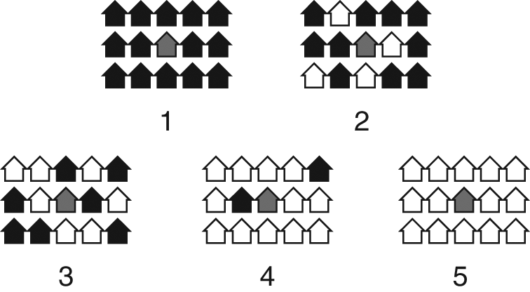
Neighborhood vignettes shown to black respondents asked about white neighbors.
These data have been analyzed using a variety of approaches, including descriptive statistics, OLS regression, and categorical response models of various types (e.g., Farley 1978; Farley et al. 1978, 1993, 1994; Charles 2000, 2005; Krysan and Farley 2002). Although these analyses have been informative, they typically do not make full use of information available in the data. In contrast to these approaches, the discrete choice models proposed in this paper make full use of the quantitative information about race-ethnic composition in these data, allow for full examination of complex interactions among race-ethnic groups, generalize to data that include more dimensions of neighborhood variation than just race-ethnic makeup, and provide a natural comparison to analyses of actual residential choices.
The MCSUI vignettes contain information only on neighborhood racial composition; all other neighborhood characteristics are ignored. Thus, it is difficult to know whether to interpret these data as representing the degree of an individual’s true ethnic “tolerance” or a response to other neighborhood characteristics (e.g., crime, school quality, and housing costs) associated with race (Quillian 1995; Harris 1999). Emerson, Chai, and Yancey (2001) use vignette neighborhoods that vary along a number of dimensions: school quality, ethnic composition, property values, and crime rate. They find that, after controlling for non-race/ethnic neighborhood characteristics, whites’ aversion to a predominantly Hispanic or Asian neighborhood is no longer statistically significant in their sample, but whites’ apparent aversion to black neighborhoods remains. Krysan et al. (2009) construct video vignettes that vary the race of actors portraying neighborhood residents, but they hold constant key visual indicators of the socioeconomic composition of neighborhoods (e.g., the upkeep of yards and the types of cars in driveways). Multidimensional vignette data in principle allow the analyst to “control for” any potential confounding neighborhood characteristics. However, it is hard to represent multidimensional neighborhoods using pictures, and complex verbal descriptions are difficult for respondents to understand. A more straightforward way of exploring how multiple factors affect residential choice is to use data on actual moves.
2.2. Mobility Histories
Residential choices and preferences may also be observed in actual mobility behavior. Information about mobility and neighborhood choice may be obtained from cross section data, such as the U.S. Decennial Census, which documents both current neighborhood of residence and also year moved into current unit (to identify recent movers). Alternatively, mobility data may come from retrospective survey questions that ask individuals to recall their previous addresses over some specified time period. For example, wave 1 of the Los Angeles Family and Neighborhood Survey (LA FANS) asked individuals to report all moves and addresses lived in over the past two years, and wave 2 asked for a residential history between wave 1 and wave 2 (Sastry et al. 2006). Residential mobility data may also be prospective, identifying respondents at the beginning of a time period and tracking their subsequent moves.
For example, the Panel Study of Income Dynamics (PSID) records where a respondent lives at the time of each interview. The population represented by a set of mobility data, of course, depends on the survey instrument. For example, the data may be nationally representative data, as in the Census or the PSID, or data focused on a particular metropolitan area, as in the LA FANS.
Several studies have used the PSID panel data to examine neighborhood mobility. Some treat the decision to move out of one’s current neighborhood (e.g., analyses of “white flight”) as a binary outcome variable (e.g., South and Crowder 1997; Rosenbaum and Friedman 2001), whereas others use the demographic (typically race-ethnic) composition of the destination neighborhood as a polytomous or quantitive outcome variable (Crowder, South, and Chavez 2006; Crowder and South 2008). The outcome is often characterized by its racial composition (e.g., its percentage of white, black, or Hispanic). Typically the outcome is modeled using a binary logit (did or did not move out) or multinomial logit (with destinations categorized into types). The goal of these analyses is to predict choice of destination conditional on individual and/or household characteristics, characteristics of the current residential census tract, and characteristics of the metropolitan area as a whole.
Although these studies usefully describe mobility among neighborhood types and covariates of this mobility, they are ill-suited to the study of residential decision-making by individuals and the impact of these decisions on segregation or other aspects of population distribution. Whereas analyses of mobility rates among neighborhoods with varying percentages of a given ethnic group examine only a single dimension of destination neighborhoods, households evaluate potential destination neighborhoods on several dimensions—for example, racial composition, economic level, housing price, and school quality—when making residential decisions. Any single dimension, when considered by itself, may be confounded with other distinct but correlated dimensions. Additionally, these studies only allow respondents’ own characteristics, characteristics of their current neighborhood, and the racial composition of the chosen tract to affect destinations, omitting the possible effects of the comparative characteristics of potential destinations on mobility decisions. As we show below, a fruitful alternative approach is to adapt models for discrete choice to the analysis of residential decision making. This approach incorporates the effects of both neighborhood and individual characteristics on residential location choice, a multidimensional approach to measuring neighborhood attractiveness, and a natural way to extrapolate to aggregate neighborhood change. Additionally, it allows us to examine both stated preferences and actual mobility decisions within a common analytic framework.
2.3. Stated Preferences Versus Mobility Histories
Stated preference (vignette) and mobility history data have several complementary strengths and weaknesses. The most important advantage of stated preference data is that the hypothetical characteristics of neighborhoods are under the control of the investigator. Thus, it is possible to assign descriptions of neighborhoods that vary along one or more dimensions to different individuals or to administer to the same individual an array of possible neighborhood configurations. Randomization combined with observations of repeated choices can control for unmeasured differences among individuals. This is a relatively low-cost means of data collection inasmuch as it does not require the collection of residential mobility histories or large samples of individuals, only a fraction of whom have moved in the recent past. It also allows for the specification of relatively rare types of neighborhoods that would otherwise require an extremely large sample of actual moves. Furthermore, stated preference designs elicit individuals’ preferences; in theory these preferences are unconstrained by affordability constraints, housing supply, discrimination, and other factors that affect actual moves.
The weaknesses of neighborhood vignettes arise because they are administered in interviews, which poorly approximate the contexts in which actual choices are made. First, preference for neighborhoods that vary in their racial makeup is potentially a sensitive subject and thus respondents may express socially desirable preferences. Second, vignettes are typically administered to individuals, but mobility decisions may be made collectively by multiple household members. Third, it is usually impractical to vary more than two or three dimensions of neighborhood desirability in vignette studies (e.g., racial makeup, poverty rate, age of housing), precluding the investigation of complex interactions among determinants of housing desirability (Harris 1999). Fourth, because neighborhood vignettes are hypothetical, stated preferences abstract from the virtually limitless array of alternatives that people may have in a real choice situation, as well as their substantial proclivity not to move (that is, to choose their current residence) as a result of the search and moving costs. Finally, as discussed further in Section 7, stated preferences may be sensitive to how interview questions are phrased.
Actual mobility histories also have their own advantages and disadvantages. On the one hand, they provide true measures of real mobility decisions, albeit subject to constraints. Additionally, because they measure choices made by heterogeneous individuals for neighborhoods that vary in a wide range of attributes, they allow the analyst to represent mobility using a rich set of individual and neighborhood covariates. Finally, probability samples of individuals and households include both movers and nonmovers and, in individual mobility histories, periods of stable residence as well as episodes of mobility. This enables the analyst to examine differences in how decision makers evaluate their own locations relative to other potential destinations, and to thus explore how origins as well as destinations affect choice.
On the other hand, actual moves are not pure measures of residential preferences. Rather, they result from preferences about desired locations in the context of constraints on residential options. If the analyst can specify the true choice set for each individual, this will reduce the extent to which constraints dominate the choice process. In practice, however, we seldom know an individual’s true range of alternatives. Additionally, mobility histories are comparatively expensive to collect. Because recent mobility is usually a relatively rare event, large amounts of data must be collected, whether through lengthy retrospective mobility histories, long prospective panels, or shorter residential histories obtained from large samples of individuals. The need for large numbers of observations is exacerbated, moreover, when the analyst wishes to look at the selection of relatively rare neighborhoods.
In principle, we can combine the strengths of stated and revealed preference data by pooling them into one model. Louviere, Hensher, and Swait (2000) discuss this possibility for studying consumer choice. To our knowledge, this approach has not yet been taken in the study of residential choice.
3. Discrete Choice Models
Discrete choice models represent behavior in which individuals choose one or more options from a set of given alternatives, typically under the assumption that they select the option(s) with the greatest utility. Ben-Akiva and Lerman (1993), Louviere et al. (2000), and Train (2003) discuss each of these models in detail. In this section we review their essential properties before discussing the special adaptations required for the study of residential mobility. Our discussion builds on the work of McFadden (1978), who first applied discrete choice models to the study of location decisions. In discrete choice models of residential mobility, the choice set may consist of housing units, neighborhoods, or other potential destinations. The outcome of interest is the specific location chosen, given the set of available alternatives. Although our discussion typically refers to the choices of individuals, in practice the choosers may be individuals, families, households, or other decision makers.
3.1. Residential Mobility as a Market Process
In most of the models discussed below, we represent residential choice as a “demand-side” process whereby individuals or households select from an array of possible destinations. This is a partial view of residential mobility inasmuch as moves in fact result from interactions between buyers and sellers or landlords and renters who negotiate the exchange of housing units. Discrete choice models capture housing demand conditional on housing supply, but these models do not represent how the actions or motivations of housing suppliers (e.g., the steering decisions of real-estate agents, the lending decisions of banks, or the building decisions of developers) affect the number and type of available units. For the limited purpose of analyzing individual choice, it suffices to assume that housing vacancies and housing prices are given and a one-sided approach is sufficient. For studying the realistic aggregate dynamics of a housing market, it may be necessary to take the supply as well as the demand side of the market into account. In later sections, we discuss how to incorporate prices into models of individual residential choice and to use price equilibrium assumptions to assess the effects of changes in aggregate demand. (An alternative modeling strategy is to model explicitly the interactions between housing suppliers and housing seekers. Such models could rely on optimal matching of housing seekers and providers [e.g., Roth and Sotomayor 1990] and use extensions of available “two-sided” statistical models for joint decisions of actors on both the supply and demand sides of a market [Logan 1996, 1998; Logan, Hoff, and Newton 2008]. Specification and implementation of such a model for housing markets is beyond the scope of this paper.)
3.2. Outcome Variable and Data Structure
In discrete choice models, the outcome is either a single choice (representing the “best” possible outcome given available opportunities) or a set of ranked choices. Rankings contain more information on preferences than single choices, which reveal the top-ranked choice but not the relative desirability of the remaining options. In data on actual choices, we typically observe only a single choice (or a series of choices made over some period of time). In stated preferences, respondents may rank neighborhoods in order of desirability. The models used to estimate parameters based on these two outcomes are similar, except that the ranked outcome model includes additional elements to the likelihood function, one for each ranking given the current set of unranked items. We discuss this in more detail below.
Table 1 shows the data structure for estimating discrete choice models. Each of the I individuals has J lines of data, one for each of potential destination alternatives. We refer to each line of data as an “individual-alternative” and the set of J alternatives as the individual’s choice set. In the example shown in Table 1, J = 5 for all individuals, but in general it is possible for the size of choice set to vary across individuals. Individual characteristics (X i ,) are constant within individuals, but features of neighborhood alternatives (Z j ), such as neighborhood proportion own-race, vary across alternatives within individuals.
Data Structure Used in Estimation of Discrete Choice Models
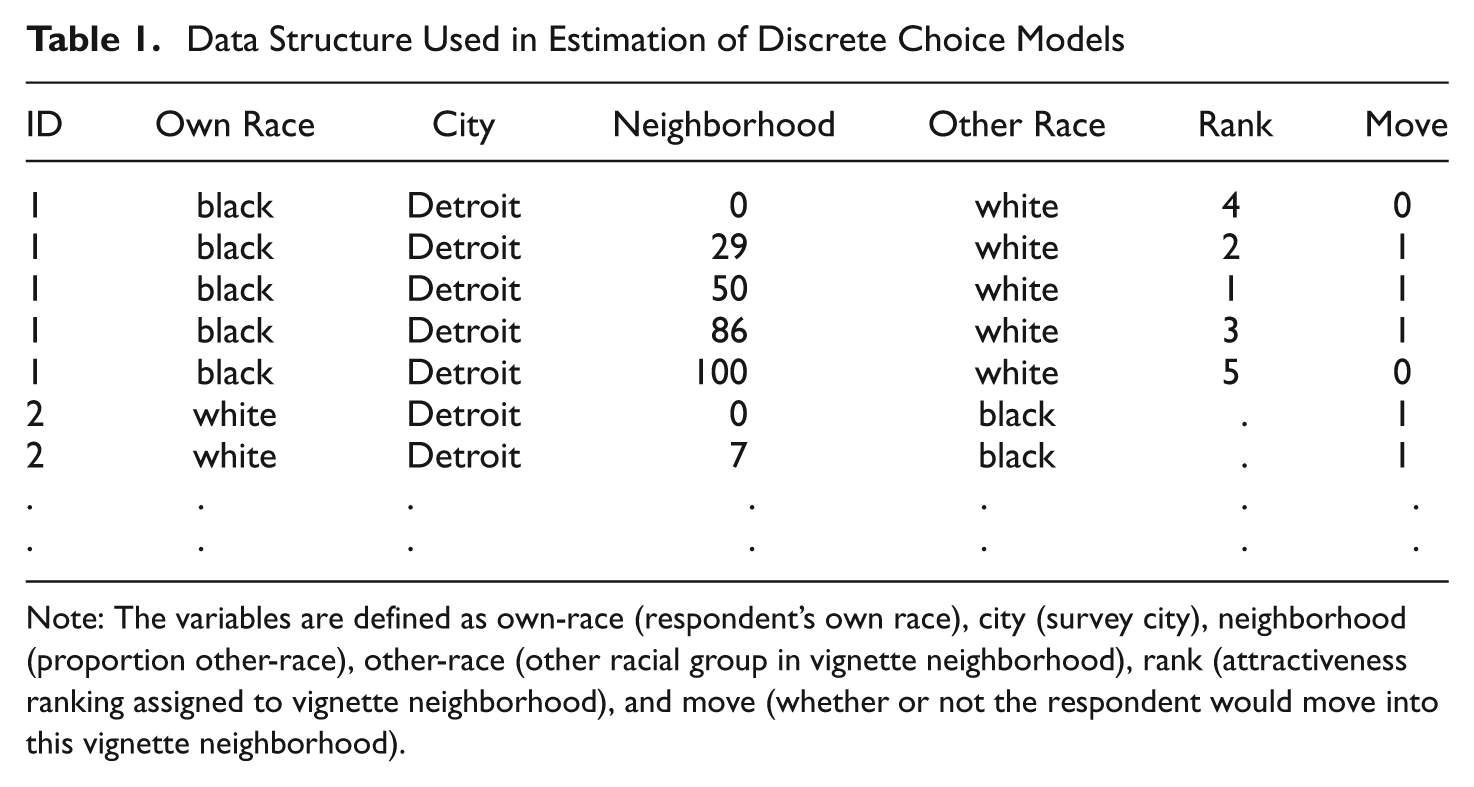
Note: The variables are defined as own-race (respondent’s own race), city (survey city), neighborhood (proportion other-race), other-race (other racial group in vignette neighborhood), rank (attractiveness ranking assigned to vignette neighborhood), and move (whether or not the respondent would move into this vignette neighborhood).
3.3. Conditional Logit Model
Let Y
ij
be an indicator variable denoting which neighborhood (indexed by j) is chosen by the ith individual (i = 1, . . ., I; j = 1, . . ., J). Let U
ij
denote the (latent) utility or attractiveness that the ith individual attaches to the jth neighborhood. Let p
ij
denote the probability that the ith individual chooses the jth neighborhood. The utility of a neighborhood for an individual depends on neighborhood characteristics, possibly interacting with characteristics of individuals. These characteristics may or may not be known by the researcher, but they are known to the individuals to whom they apply. Let

If F is a linear random utility model, then, for example, for a single observed neighborhood and personal characteristic (Z and X respectively), the model is

where β and γ are parameters to be estimated. When individuals choose where to live, they implicitly compare neighborhoods in their choice set—that is, neighborhoods that they know about and where they may move with a nonzero probability. The difference in utility between the jth and the kth neighborhood is

Utility differences among neighborhoods for a given individual are thus a function of differences in observed and unobserved characteristics of neighborhoods and individuals. Because utility comparisons take place within individuals, their characteristics X i do not affect the utility comparison additively. These characteristics, however, may interact with neighborhood characteristics. For example, the effect of differences in the proportion of persons in a neighborhood in a given ethnic group on the relative attractiveness of the neighborhoods may differ between individuals who are members of that ethnic group and those who are not. Unmeasured characteristics of individuals may also modify the effects of neighborhood characteristics, as we show below. These unmeasured characteristics can induce random variation in the effects of measured neighborhood characteristics β. For example, the effect of the proportion of persons in the neighborhood who are ethnic minorities may depend on an individual’s level of tolerance, which is unobserved to the analyst.
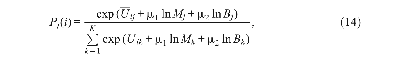
Given data on the characteristics of individuals and neighborhoods and the behaviors or stated preferences of individuals for neighborhoods and an assumed probability distribution of the unobserved characteristics of individuals and neighborhoods, it is possible to estimate the parameters of the discrete choice model. If the φ ij follow a type I extreme value (Gumbel) distribution, we obtain the conditional logit model 2

where C (i) denotes the choice set for the ith individual, which may be restricted to incorporate discrimination, prices, or information constraints (McFadden 1978). 3 For example, the choice set may be restricted to units within a given radius of a person’s current home, to units in neighborhoods that are at least 10% own-race, or to units where monthly rent or mortgage payments would be less than some fraction of individuals’ incomes. Typically these models are estimated using maximum likelihood, where the likelihood is

Early applications of the basic discrete choice model to residential mobility analysis include McFadden (1978) and Lerman (1975). Gabriel and Rosenthal (1989) use a multinomial logit model to examine how race and other traits of individuals affect residential mobility among five counties in the Washington, D.C., area. Sermons and Koppelman (2001) estimate a discrete choice model of residential choice that explores how men and women differ in their sensitivity to commuting time. 4
3.4. Independence from Irrelevant Alternatives Assumption
The conditional logit form of the discrete choice model assumes independence from irrelevant alternatives (IIA). It is a model for pairwise comparison and assumes that the odds of preferring an alternative in a pairwise comparison is unaffected by the other available alternatives. That is, after accounting for observable features of choices, the remaining (unobserved) features of choices are uncorrelated (that is,
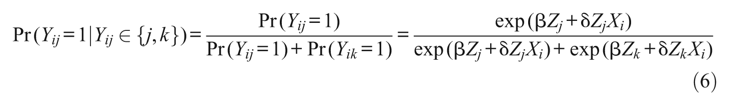
This probability does not depend on the traits of neighborhoods other than j and k. If valid, this assumption makes it possible to estimate choice models on a subset of alternatives in the choice set. Additionally, we can make out-of-sample predictions because the parameter estimates from the model are invariant to the inclusion or exclusion of alternatives in individuals’ choice sets.
However, in practice the IIA assumption is often not met. We rarely observe all attributes of destinations that affect mobility behavior. Some neighborhoods have similar characteristics and, if one of them were omitted, individuals would disproportionately choose a similar neighborhood rather than distribute themselves proportionately across both similar and dissimilar neighborhoods. Unless the sources of similarity and dissimilarity among neighborhoods are controlled in the choice model, the model is likely to yield incorrect predictions about the effects of omitting one of the neighborhoods. The most common way of testing for IIA is through partitioning the choice set, and comparing estimates from a full model with those from a model estimated using a subset of the choice set (Hausman and McFadden 1984; Small and Hsiao 1985). 5
There are three ways of dealing with IIA violations. First, we can ignore violation of the IIA assumption but recognize that the estimated parameters are at best an approximation of choice behavior and are not appropriate for making inferences about substitution patterns. Second, we can in principle modify the discrete choice model by adding additional covariates that represent sources of neighborhood resemblance. However, usually we cannot capture all the unobserved correlation in choice behavior explicitly. Finally, if available data permit, we can use a mixed logit specification, preferably with panel data that permit identification of unobserved time invariant neighborhood heterogeneity. We discuss these models in more detail below.
3.5. Unmeasured Heterogeneity
Even neighborhoods that are identical on measured characteristics may vary in their desirability to individuals. For example, neighborhoods may vary in amenities that have not been measured (nearness to the ocean or availability of charming coffee shops). Additionally, even among individuals who have identical measured attributes, we may observe variation in their mobility behavior. Unaccounted for features of individuals or neighborhoods that affect choice behavior can lead to correlations in the disturbance φ ij across alternatives. Another form of unobserved heterogeneity arises if we incorrectly assume that people select one neighborhood directly from a given choice set when in fact they decide sequentially, systematically narrowing down their options based on some criterion. For example, choosers may first select part of a city, then select a neighborhood within that part, and then a house within the neighborhood. In this case, all neighborhoods within the chosen region and all vacant houses within the chosen neighborhood have a higher than average probability of selection irrespective of their measured characteristics. When the number of alternatives is small, we can represent the average level of attractiveness of each residential choice by including alternative-specific constants, which enter as dichotomous variables in the choice model. However, when the choice set is large, when we seek to parameterize the effects of measured attributes of neighborhoods on choice probabilities, or when the concern is with unobserved attributes of individuals that influence choice behavior, it is more appropriate to estimate a model that allows for correlation in the attractiveness of observations within or among individuals. Several models are available to represent correlation of attractiveness across observations, including the nested and mixed logit models. We discuss these in turn.
3.5.1. Nested Logit Models
Nested logit models may solve the problem of unmeasured neighborhood heterogeneity if unmeasured characteristics of alternatives can be accounted for by conditioning on the appropriate choice subset. For example, if the choice set is all neighborhoods within the Detroit Metropolitan Area, but all the neighborhoods within the Grosse Pointe area of Detroit share key attributes (zoning regulation, funding for schools, etc.), at least some of which are unmeasured, we can treat Grosse Pointe neighborhoods as a subset. Subsets or “nests” are alternatives that are similar along one or more dimensions not accounted for in the formal discrete choice model. The nested logit model partitions the choice set C into N“nests,”C
n
such that the complete choice set
The nesting structure assumes that (1) neighborhoods that are in the same nests share unobserved features and (2) neighborhoods across nests do not share these unobserved features. That is, choices may have correlated unobservables within nests but not between them. 7 Whereas in the simple conditional logit model, disturbances are independent and follow a univariate extreme value distribution, in the nested logit the marginal distribution of the disturbances across nests follows a univariate extreme value distribution but the disturbances may be correlated within nests (Train 2003, Ch. 4). To estimate the nested logit model, the nesting structure must be known to the analyst in advance, which is often not the case. 8 Resemblance of alternatives on unobserved traits for any subset of alternatives, moreover, is often not an all-or-nothing matter but rather a matter of degree. These considerations give rise to the need for a more flexible model for unobserved heterogeneity.
3.5.2. Mixed Logit Model
Mixed logit models are a more general class of models that can accommodate both alternative- and individual-specific unmeasured heterogeneity, and they are useful if the analyst believes that the unobserved heterogeneity is correlated with observable characteristics of neighborhoods. The model is an extension of Equation (4). In particular, the error component φ ij is broken out into two parts; that is,

where μ
i
is an individual-specific (alternative invariant) random vector with zero mean, the W
ij
are one or more vectors of data related to the jth alternative, and

where V(µ) is the covariance matrix for µ. Given some value µ i , the conditional choice probability follows the logistic distribution since the remaining error component ε ik follows an extreme value distribution:
Because the µ i are unobserved, the unconditional probability is the logit formula integrated over all possible values for µ i , weighted by the density of µ.

where Ω denotes support for the distribution of µ. These models are referred to as “mixed logit” because their probabilities are heterogeneous with f as the mixing distribution (Train 2003). The mixing distribution is assumed by the analyst, and it can be normal, lognormal, or other shapes. Because choice probabilities do not have closed form solutions, they cannot be estimated directly. Instead, the probabilities can be simulated by drawing values of µ, from its assumed distribution, using a Gibbs sampler, EM algorithm, or some other form of iterative estimation (see Train 2003, Chs. 8–10). These models can be estimated using specialized software for discrete choice estimation, such as the NLOGIT package for LIMDEP.
The choice probabilities depend on parameters β, γ, and Ω. Different patterns of correlation are specified based on the choice of W
ij
. For example, in the nested logit model with N nests, W
ij
is a set of dummy variables,
If the pattern of unobserved heterogeneity across alternatives is unknown, the W
ij
can be specified as error components that, along with ε
ij
, make up the random component of utility. In the usual conditional logit model, W
ij
are zero, which means there is no correlation in utility over alternatives after conditioning on observables. When
Because this specification includes no measured neighborhood characteristics to identify the correlation across observations, it requires strong assumptions about the distribution of the W ij random deviates.
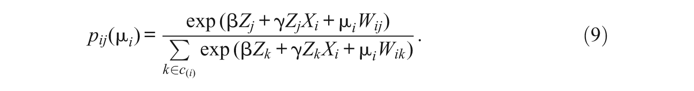
Mixed logit models can also represent heterogeneity in individual behavior by assuming that Wij= Z (or Zj X
i
when the random coefficient refers to interaction between alternative- and individual-specific variables) such that
While mixed logit models are widely used in transportation and land-use research, there are only a few studies that apply them specifically to the analysis of residential choice. In their analysis of Dallas County households’ choices to live in a particular land-use zone, Bhat and Guo (2004) estimate a mixed spatially correlated logit that allows for both unobserved taste variation among movers and also spatial correlation among adjacent zones. More recently, Hoshino (2011) uses a mixed logit model to analyze stated preference data collected in Tokyo.
3.5.3. Estimating Unobserved Heterogeneity in Alternatives with Repeated Measures Data
When the goal is to estimate unobserved heterogeneity across individual movers, or when the correlation in unobservables across alternatives is well defined (for example, in the nested logit specification and other special cases), the mixed logit model is an elegant way of parameterizing unobserved heterogeneity in the choice model. If we believe that there is unobserved heterogeneity across alternatives but do not know the structure of this heterogeneity, the model is not generally identified.
If, however, we observe more than one choice by at least a subset of individuals, identification can be achieved. A typical form of repeated measures comes through panel observations, in which individuals make repeated decisions about whether and where to move. This requires that we observe the same individuals making mobility decisions over a period during which observable characteristics of neighborhoods change. This enables the analyst to control for unobserved time-invariant characteristics of alternatives (e.g., proximity to beach or neighborhood history). With repeated measures, either fixed effects or correlated random effects specifications are available. The fixed effects specification is tantamount to incorporating a dummy variable for every alternative. The random effects specification assumes a distribution for the unobservables but uses the assumed time invariance of the distribution to identify its correlation with time-varying characteristics of the alternatives. These models are applications of standard methods for discrete response models with panel or other clustered data (Chamberlain 1980; Maddala 1983). Equivalently, discrete choice models with unmeasured heterogeneity and repeated measures can be regarded as a species of multilevel model, in which the levels include individuals, alternatives in the choice sets of individuals, and time-specific alternatives. Issues of identification and estimation of these models for residential choice parallel those for the general multilevel model. (See Skrondal and Rabe-Hesketh [2004] for a more detailed discussion of discrete choice models with unmeasured heterogeneity and their relationship to other multilevel models.)
3.6. Functional Form
Discrete choice models allow the analyst to specify a variety of ways that people may respond to characteristics of neighborhoods. For example, in models of the relationship between neighborhood racial composition and the probability of entering or leaving a neighborhood, it is not just the average level of tolerance that matters but also the shape of the response curve. Schelling (1971, 1978) showed that a high level of segregation results when individuals have a threshold response to the proportion own-group in their neighborhood—that is, when people are indifferent to neighborhood characteristics within some interval and only care about whether a neighborhood characteristic is above or below the threshold. In a simple model where only neighborhood characteristic Zj enters into the choice equation, the utility in a threshold specification is

where the threshold is a specific value of Zj. An alternative behavioral response is that people have a continuous response to neighborhood composition; in other words they are sensitive to even small changes in composition regardless of the actual level of the compositional variable. That is, utility is a continuous specification of neighborhood composition—for example,
3.7. Models for Ranked Data
The discrete choice models discussed thus far assume that the analyst observes only the chosen alternative and has no information on the relative utilities of unchosen alternatives. Stated preference data, however, may provide information on full or partial ranking of alternatives, albeit for a hypothetical choice set (Allison and Christakis 1994). 9 Ties occur in the data when respondents assign multiple items the same rank, and incomplete rankings occur when respondents leave certain items un-ranked. In this case, we observe groups of items that are ranked together, providing a partial ranking. The rank-ordered logit accommodates tied rankings (Allison and Christakis 1994:206–8). The likelihood function is an extension of the simpler discrete choice likelihood Equation (5), except that Y ij is a rank rather than a 0/1 indicator for the chosen alternative, and the model includes an additional term δ ijk , which equals 1 if the ranking of the kth choice is greater than or equal to the ranking of the jth choice, and is zero otherwise. That is,

In the case where one alternative is ranked “first” and all others are tied for “last,” the rank-ordered logit model simplifies to the discrete choice model for a single choice.
4. Complications for Actual Choice Data
In this section we discuss features of residential choice data that require modifications of standard discrete choice models. These include the aggregation of alternatives, violations of the independence from irrelevant alternatives assumption, unfeasibly large choice sets, choice-based sampling, and the treatment of a respondent’s current place of residence. We discuss how each of these problems can be handled within the choice model.
4.1. Aggregation of Alternatives
In actual residential choice, individuals select among housing units, apartments, or even rooms. Typically, however, we observe choices of aggregate units such as Census tracts. When the units that individuals actually choose are not the ones that we observe, it is necessary to modify the choice model to take into account the differential size and variability of the aggregate units (Ben-Akiva and Lerman 1985, Ch. 9). Denote by L the actual choice set (e.g., housing units). P
i
(l) is the probability that the ith decisionmaker chooses the lth housing unit (where

An implication of this result is that, all else being equal, aggregate utilities and choice probabilities vary with the size of the aggregate units. Census tracts with more housing units will, ceteris paribus, be chosen more often than those with fewer units. Further, within tracts, individual dwelling units may be heterogeneous in their desirability. Thus, the estimated effects of other measured characteristics of tracts may be distorted by their correlations with tract size and variability. To take these complications into account we modify the general choice model in Equation (4) as follows:
where
4.2. Large Number of Potential Destinations
When the residential choice set is all neighborhoods or housing units in a city or other large area, the number of observations can be very large in a discrete choice model, making it computationally burdensome to compute choice probabilities for every individual-alternative observation. For example, a discrete choice model for 1,000 individuals (and their location decisions) in a metropolitan area of 2,000 Census tracts has 1,000*2,000 = 2,000,000 individual-alternative combinations (if each tract is in the choice set of every sampled individual). Such a large data set makes computation difficult. However, we can obtain consistent estimates of the discrete choice model by sampling from the individual-destination observations within each respondent (McFadden 1978; Ben-Akiva and Lerman 1985). This procedure can be accomplished without significant loss of information, if we use all information on actually chosen alternatives and a random subsample of unchosen alternatives. This is analogous to the procedure of subsampling the risk sets in survival analysis (e.g., Breslow et al. 1983) or subsampling controls in case-control designs (Jewell 2004). If we subsample unchosen alternatives, it is possible to estimate a modified version of the model shown in Equation (4), which is
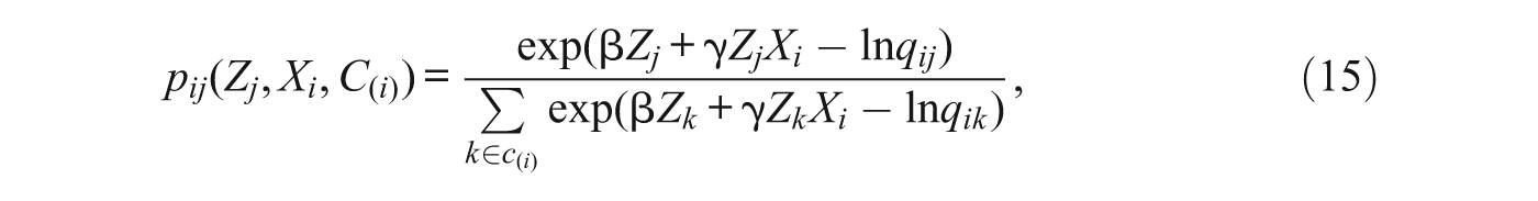
where q ij denotes the known probability of sampling thejth destination for the ith respondent. We sample according to the following rules:
If the alternative is chosen, sample with q ij = 1.0.
If the alternative is not chosen, sample with q ij << 1.0.
For example, if we sample the unchosen alternatives with probability 0.05, this procedure yields a sample of 1,000 + (1,999 × 1,000) × 0.05 = 100,950, a more manageable number of alternative-individual observations. This model can be estimated using standard maximum likelihood approaches for the discrete choice model, subject to the constraint that the coefficient on q ij is 1.0. In practice, there are no firm guidelines for selecting a value of q ij . The value will depend on both the sample size and also the size of the choice set. However, the computational burden of estimating the choice model is linear in both the number of observations and the number of alternatives. Thus if we have sufficient observations, it is more fruitful to analyze a sample of many observations with a small number of sampled alternatives rather than fewer observations with a large number of alternatives (Ben-Akiva and Lerman 1985:263). In practice, we can do sensitivity analyses to determine how alternative subsampling probabilities affect the estimated coefficients and standard errors. For example, we can vary the subsampling fraction and pick the smallest fraction that does not result in marked loss of precision of estimates.
4.3. Choice-based Sampling
Many surveys employ a form of stratified sampling that overrepresents some kinds of neighborhoods and underrepresents others. For example, surveys may oversample poor neighborhoods within a city or be drawn from schools or school districts with atypical minority or socioeconomic representation. Whereas this stratification scheme may be exogenous for some analytic purposes, it results in endogenous stratification for the study of neighborhood choice. Neighborhood stratified samples, therefore, are choice-based (Manski and Lerman 1977), in that the sampling procedure is confounded with the residential choices of the respondents. Without correction for sample design, estimates of parameters in discrete choice models are not, in general, consistent. If choice-based sampling probabilities are known, however, we can obtain consistent estimates of the model parameters using sampling weights. Manski and Lerman (1977) introduce an estimator in which each observed residential choice is weighted by its representation in the population as a whole. We define a function for each respondent,

where Vi denotes the population shares and H i denotes the sample shares for that respondent’s type. These weights enter the likelihood function for the model as

In practice, the correction weights for choice-based sampling can be estimated using the “importance weights” option in statistical estimation packages. For example, consider a sample of households where the proportion of respondents in high-poverty neighborhoods (≥30% of households below the poverty line) and low-poverty neighborhoods (<30% of households below the poverty line) are each 0.5, whereas the population proportions of households in high- and low-poverty neighborhoods are 0.3 and 0.7, respectively. In this case, the Manski-Lerman weights are 0.3/0.5 for respondents in high poverty tracts and 0.7/0.5 for respondents in low poverty tracts.
4.4. Nuances of Behavior
4.4.1. Treatment of Own Neighborhood
In most populations the most common choice that an individual makes is his or her own residential location—that is, the choice not to move. This tendency to stay put may be due to the costs of moving as well as familiarity and comfort with the current location. Nonmoves are informative about residential choice because it is likely that the chances of opting for one’s own neighborhood do in fact depend on the measured characteristics of the neighborhood. Models of residential choice, however, should take into account the possibility that the weights that individuals place on neighborhood characteristics may be different for their own neighborhoods than for other potential destinations. We can represent the differential treatment people give to their own housing units or neighborhoods in the choice model by including a dichotomous variable, D ij , that equals 1 if the housing unit or neighborhood under consideration is the respondent’s current residence and 0 otherwise. D ij can enter into the model alone, which allows for a tendency not to move, or in interactions with characteristics of individuals or neighborhoods, which implies the differential own neighborhood by individuals with varying characteristics or differential evaluation of characteristics of own neighborhood. We illustrate how D ij is used Section 7.
4.4.2. Neighborhood Change Versus Neighborhood Levels
Mobility history data can also show the extent to which people respond to neighborhood change, above and beyond their response to static compositional levels. Expectations regarding future changes in population composition and housing prices are important factors that may be based on recent changes in these conditions and may affect individuals’ mobility decisions. An expectation of continuing trends may create a self-fulfilling prophecy, where neighborhoods that are believed to improve or decline may in fact change in these directions because people act on these beliefs. These ideas are easily incorporated into the discrete choice model by including variables that represent changes in neighborhood characteristics (that is, recent change in the Z j ), provided such data are available.
4.4.3 The Effect of Experience
Individuals’ preferences may change as a result of their prior residential experiences, and this may affect their residential choices. When panel data on residential mobility or retrospective residential histories are available, the analyst observes multiple choices made by each decision maker and variation within as well as between individuals in exposure to different kinds of neighborhoods. If the unobserved component of utility is uncorrelated within people over time, we can treat each period as independent and analyze the longitudinal observations in the same way as cross-sectional data. In models estimated from these data, including covariates from other time periods can capture dynamic aspects of behavior. For example, a measure of the race-ethnic composition of individuals’ previous neighborhoods, possibly interacted with the current neighborhood’s race-ethnic composition, may reveal how past exposure to integrated or segregated neighborhoods can affect later decisions. However, the assumption that the unobserved component of utility is uncorrelated over time within people may not hold because some unobserved factors that affect choices persist over time. Moreover, if observable factors evolve over time, then unobserved factors may also be changing in a nonrandom way. For further discussion of how to separate enduring unobserved factors that affect choices from “habit formation” and other forms of inertia or persistence in discrete choice models, see Abbring (2010), Carro (2007), and Heckman and Navarro (2007).
5. Complications for Stated Preference Data
In this section, we discuss potential issues for the analysis of stated preference data. With stated preference data, some of the complications created by mobility histories are avoidable, although other problems may arise. Typically the choice set observed in stated preference data is relatively small (e.g., five neighborhood vignettes in the MCSUI data), so choice-based sampling does not occur and the units of analysis are well defined. Although survey data on stated residential preferences typically do not offer respondents the option of choosing their own neighborhood, in principle, there is no obstacle to incorporating such measures in vignette designs. If the vignette data contain a choice that represents the respondent’s current residence, we can explore whether the characteristics of one’s own neighborhood have different effects from those of other potential destinations. Similarly, if the preference data are from a panel, it is possible to estimate models that allow for preferences to evolve over time.
However, discrete choice models based on stated preferences may, like those based on actual choices, be subject to unmeasured individual and location specific heterogeneity. Although randomized designs in stated preference studies eliminate correlation between unmeasured individual characteristics and exposure to neighborhood types, these designs cannot rule out interactions between unobserved individual characteristics and measured neighborhood characteristics. Moreover, whereas some characteristics of neighborhoods are observed by design, respondents may impute additional dimensions of neighborhood composition based on the characteristics shown in the vignette. For example, if vignette neighborhoods vary in their ethnic composition, respondents may make assumptions about other aspects of neighborhood quality (such as safety and schools) that are correlated with ethnicity (Harris 1999). This leads to the same specification error that occurs when there is unobserved heterogeneity across neighborhoods in the actual move data. Whereas it is relatively straightforward to incorporate individual-level heterogeneity into stated preference models (e.g., by adding additional covariates or incorporating random coefficients using a mixed logit approach), allowing for unobserved heterogeneity in hypothetical alternatives is not possible. A potential solution is multidimensional vignettes (Emerson, et al. 2001), although respondents may find it difficult to respond to hypothetical multidimensional choices.
A problem specific to stated preference data is ambiguity in how respondents interpret vignette questions. The MCSUI asked three questions: (1) Would you move into/out of a neighborhood? (2) What is the relative attractiveness of each neighborhood? and (3) What is your ideal neighborhood? Responses to “Would you move into this neighborhood?” may yield different results from those to “Would you move out of this neighborhood?” Because people may evaluate their own neighborhood differently from other potential destinations, these two questions may not elicit the same stated preferences. Beyond this, the three questions may be measuring distinct aspects of preferences. The “would move in/out” provides a measure of the desirable neighborhoods above some acceptability threshold; the “ranked attractiveness” question provides a full ranking of neighborhood desirability; and the “ideal neighborhood” question measures the most desirable neighborhood in a multiethnic context. However, relative “attractiveness” of neighborhoods may not dictate the relative likelihoods that respondents would in fact choose those neighborhoods. The ideal neighborhood question allows the respondent to create a neighborhood rather than respond to prespecified proportions in a given ethnic group. If IIA holds, we can compare these preference data to those from different choice sets (including the two-race neighborhoods used in the other MCSUI vignettes). However, it is not clear whether a respondent’s “ideal” neighborhood is also his or her “most attractive” neighborhood. These problems do not reduce the value of the MCSUI and similar data for understanding racial preferences, but they imply that we must be careful in interpreting the results from each question type.
6. Prices and Markets
Residential choices are made in the context of housing markets and are thus constrained by limits to information, prices, incomes, and other institutional barriers. Actual move data are not a true measure of residential preference because they reflect the combined effects of preferences and constraints. If the analyst knows what informational constraints limit the choices of specific households, such constraints can be accommodated via restrictions to the choice set. Typically, however, we do not know what options an individual considers, although it may be possible to document the different housing search strategies used by different race-ethnic groups or survey respondents’ willingness to search for housing in specific areas (Krysan 2008; Krysan and Bader 2007). Affordability constraints can be incorporated into the choice model using measures of housing costs and the individual’s economic resources. By itself, however, this approach assumes that housing prices are exogenous characteristics of dwelling units or neighborhoods. From the standpoint of modeling the marginal effect of neighborhood or housing characteristics, this assumption may be valid. Because prices are sensitive to housing demand, however, they are unlikely to be exogenous in the aggregate. The endogeneity of prices must be taken into account when we attempt to extrapolate individual behavior to aggregate population change.
6.1. Housing Markets and Housing Prices
Although housing prices affect choice behavior, the estimated effects of prices may be contaminated by factors omitted from the model that affect neighborhood desirability and thus also affect demand for housing in an area and housing prices. Estimating discrete choice models that include housing costs without taking into account this problem of unmeasured sources of desirability will result in inconsistent parameter estimates. In linear models, a possible solution is to use instrumental variables to eliminate correlation between the error term and covariates. However, discrete choice models are more complicated because of the nonlinearity of the model and possible interactions between the characteristics of individuals and the characteristics of their potential choices. To address these problems, Berry (1994) and Berry, Levinsohn, and Pakes (1995) estimate a series of alternative-specific constants that capture average demand for different alternatives (based on both observed and unobserved characteristics) and incorporate them into a conditional logit or mixed logit model. When applied to neighborhood choice data, the alternative-specific constants absorb the unobserved component of neighborhood desirability. This removes the simultaneity problem that arises out of correlation between prices and unobserved features of neighborhoods in models of individual choice.
This approach decomposes unobserved determinants of neighborhood choice into (1) the average utility that individuals derive from unobserved neighborhood characteristics

where pj denotes the average house price in the jth neighborhood. The negative coefficient indicates that neighborhood utility varies inversely with housing prices, all else being equal. The endogeneity problem is that prices depend on both observed and unobserved attributes of neighborhoods that affect desirability and thus demand. In other words, prices are a function of ξ j . The solution is to introduce a constant for each neighborhood that captures its average utility (based on both observed and unobserved characteristics). This moves ξ j out of the error term and into this alternative specific constant. Rearranging terms in (18), we have

where the term in brackets does not vary over individuals. If we denote the alternative specific constants as

This choice model no longer has an endogeneity problem because ξ j are subsumed into the alternative specific constants, which can be estimated along with the other parameters of the model. (We present this solution for the standard conditional logit model, but this strategy can also be applied to other models, including the mixed logit model). This model provides estimates of the alternative specific coefficient and the remaining parameters for choice behavior. However, the parameters associated with the utility for a given neighborhood that is common to all individuals remain subsumed in the δ j . Fortunately, because these parameters enter the definition of the alternative specific constants linearly, they can be treated as outcomes in a regression model where the dependent variable is the alternative specific constant and the explanatory variables are characteristics of the neighborhood, including price. Here ξ j is endogenous, but there are well-developed IV procedures for handling endogeneity in a linear model. The practical problem with this approach is that when the number of alternatives is large it is not feasible to estimate the alternative specific constants. Berry et al. (1995) provide an algorithm for estimating these parameters when there is a large number of alternatives.
Bayer and colleagues (Bayer and McMillan, 2008; Bayer, McMillan, and Rueben 2004) use this method in their analyses of residential choice and segregation dynamics. To obtain consistent estimates of the relationship between housing costs and mobility behavior, they divide their discrete choice utility function into a house-specific fixed effect, δ
j
, and individual-specific interaction component, λ
ij
, such that
7. Examples
7.1. Stated Residential Preferences in MCSUI Data
We illustrate the analysis of stated preference data using the MCSUI data for Los Angeles. For illustrative purposes, we analyze only the “ranked attractiveness” and “would move in” data. The ranked-attractiveness data were collected only for nonwhite respondents. Table 2 shows the percentage of neighborhoods that were ranked first or second by black, Asian, and Hispanic respondents who were asked about neighbors of different race-ethnicities. Among black respondents asked about white, Asian, or Hispanic neighbors, the most attractive neighborhoods were those with a minority of other-group neighbors. However, a nontrivial proportion of black respondents identified the entirely other-group neighborhood (e.g., 100% white) as the most attractive neighborhood. Asian respondents were also most likely to rank neighborhoods with a minority of other-group neighbors as most attractive, although they found Hispanic and black neighbors less attractive than white neighbors. Similarly, Hispanic respondents found white neighbors more attractive than black or Asian neighbors but were most likely to rank neighbors with a strong Hispanic presence most attractive.
Percentage of Neighborhoods Ranked First or Second, by Respondent’s Ethnicity and Percentage Other in Neighborhood
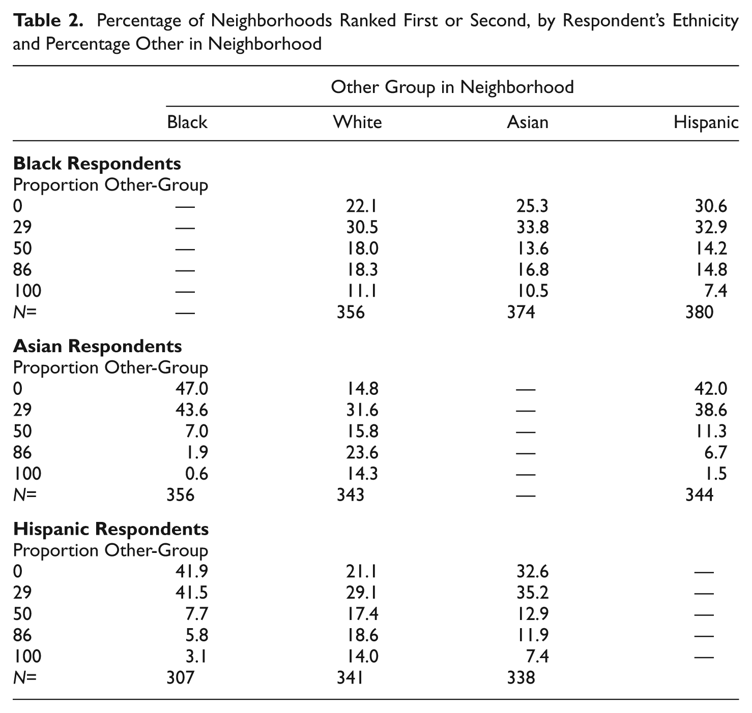
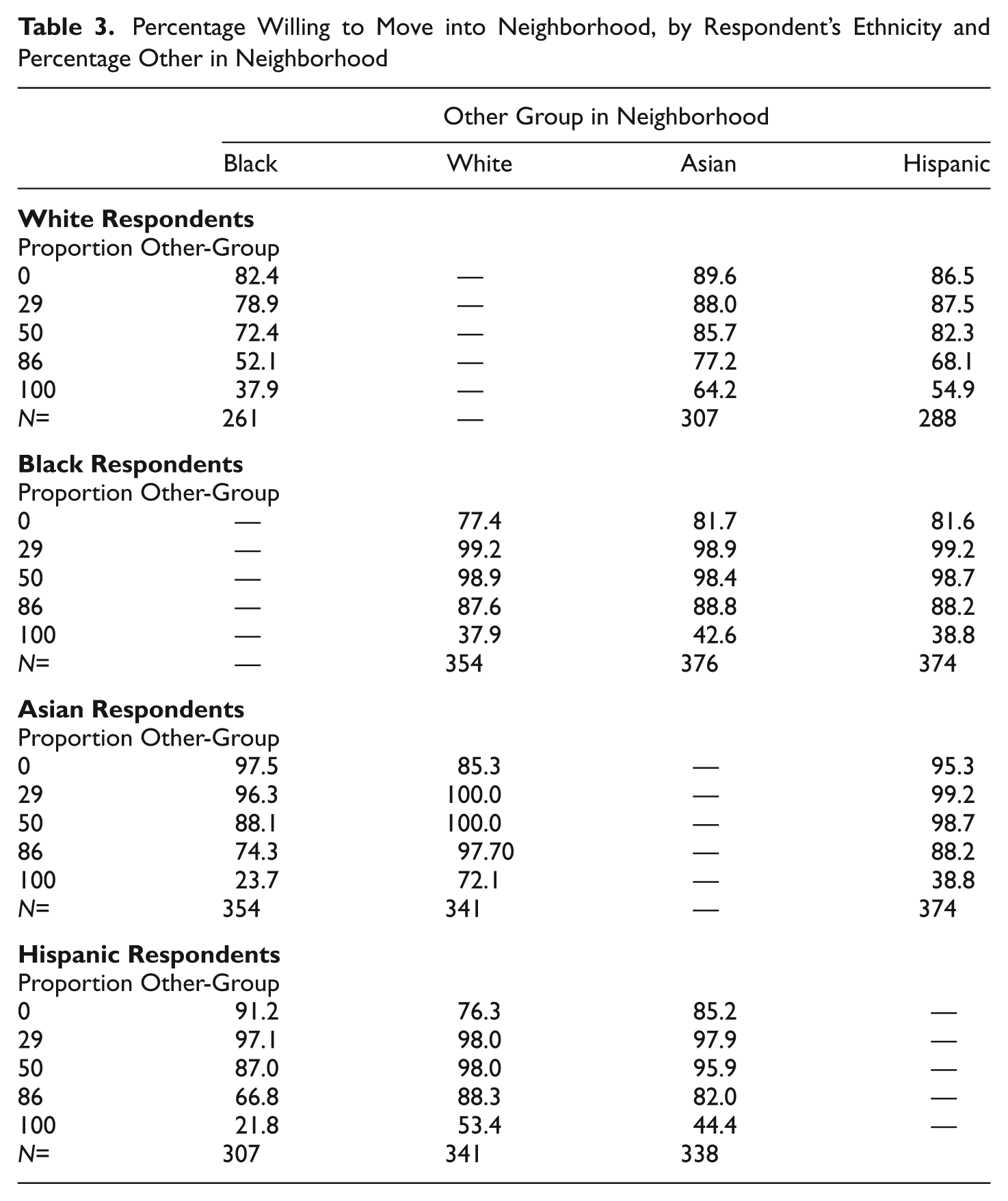
Table 3 shows the percentage of white, black, Hispanic, and Asian respondents willing to move into a neighborhood based on its neighborhood proportion other (where the other-group may be white, black, Asian, or Hispanic). The first column of the table, which shows how white, Asian, and Hispanic respondents evaluate black neighbors, indicates that all groups avoid majority black neighborhoods. These descriptive tables show the distribution of responses over categories of neighborhood proportion other, but they do not provide a succinct way of showing the relationship between neighborhood preferences and neighborhood characteristics.
Percentage Willing to Move into Neighborhood, by Respondent’s Ethnicity and Percentage Other in Neighborhood
7.1.1. Models
We analyze the “ranked attractiveness” data by treating the five responses (one for each vignette neighborhood) as a full ranking of the alternatives. In contrast, we treat the five responses to the “would you move in/out” question as a partial ranking of the alternative vignette neighborhoods, and use these rankings to estimate rank-ordered logit models with ties. In Table 1 each respondent has five lines of data, one for each neighborhood ethnic composition vignette and the respondent’s rank of the vignette. The vignette rank is the dependent variable and is modeled as a function of the percent other-group in the neighborhood. 11 Separate parameters are estimated for each combination of a respondent’s own race and the race of the other group in the vignette neighborhood. The nonlinear continuous model adequately describes residential preferences for these simple data. The coefficients from these models are shown in Table 4.
Coefficients for Neighborhood Proportion Other Group on Residential Preferences, Neighborhood Attractiveness and Would Move In Questions, Nonlinear Continuous Functions
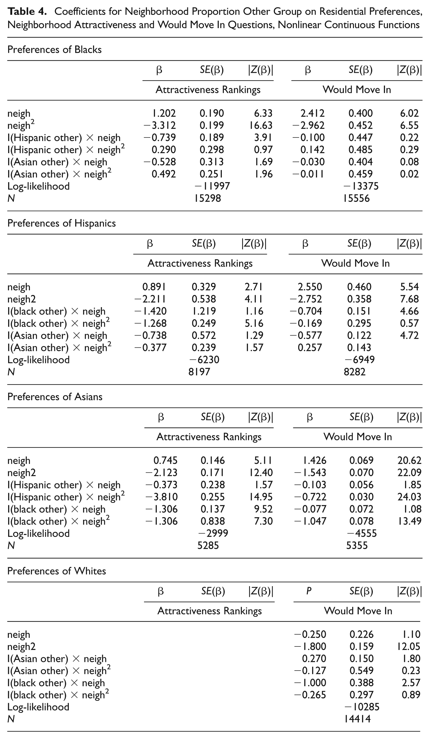
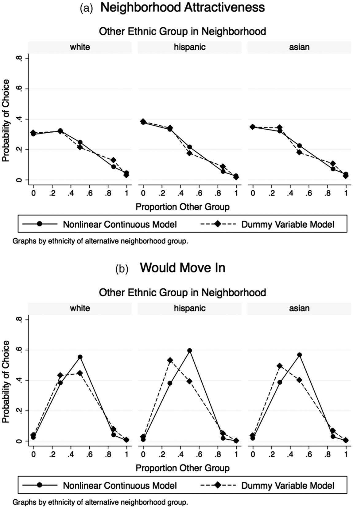
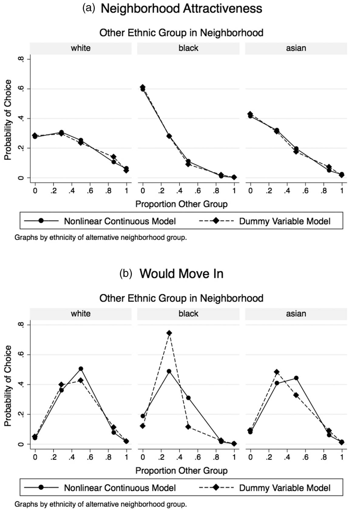
The predicted probabilities from the models for two of the ethnic groups, blacks and Hispanics, are presented in Figures 2 and 3. Figure 2(a) shows the probability that black respondents rank a vignette neighborhood most attractive. Separate panels are shown for black-white, black-Hispanic, and black-Asian neighborhoods. Black respondents tend to rank as most attractive those neighborhoods where their own ethnic group is heavily represented most. However, when asked which neighborhoods they would be willing to move into, blacks display a strong preference for integrated neighborhoods. Blacks are also slightly more partial to white neighbors than Hispanic or black neighbors; they respond to all three groups in a similar way for both the neighborhood attractiveness and “would move in” questions. Figure 3 shows the corresponding response profiles for Hispanics. Like blacks, Hispanics tend to find neighborhoods where their own group is heavily represented more attractive. However, unlike blacks, Hispanics tend to respond to mixed neighborhoods differently depending on the ethnicity of the other group. Hispanics find black neighbors least attractive. Hispanics are most likely to move into diverse neighborhoods.
Predicted probabilities for black respondents, nonparametric (dummy variable) and nonlinear continuous models.
Predicted probabilities for Hispanics, nonparametric (dummy variable) and nonlinear continuous models.
7.1.2. Unobserved Heterogeneity
Within race-ethnic groups, individuals vary in their residential preferences and their expressed tolerance of other groups. To allow for unobserved heterogeneity within race-ethnic groups, we estimate a set of latent class models allowing for a distribution of responses to neighborhood composition within each ethnic group. This is a specific instance of the mixed logit model discussed above, where

In our example below, we use the ranked-attractiveness data to estimate separate models by respondents’ race and by the race of their vignette neighbors. We estimate a nonparametric model with dummy variables for each vignette neighborhood (omitted category is the 100% own-group neighborhood). Here Z
j
is a set of dummy variables that identify vignette neighborhoods, so that
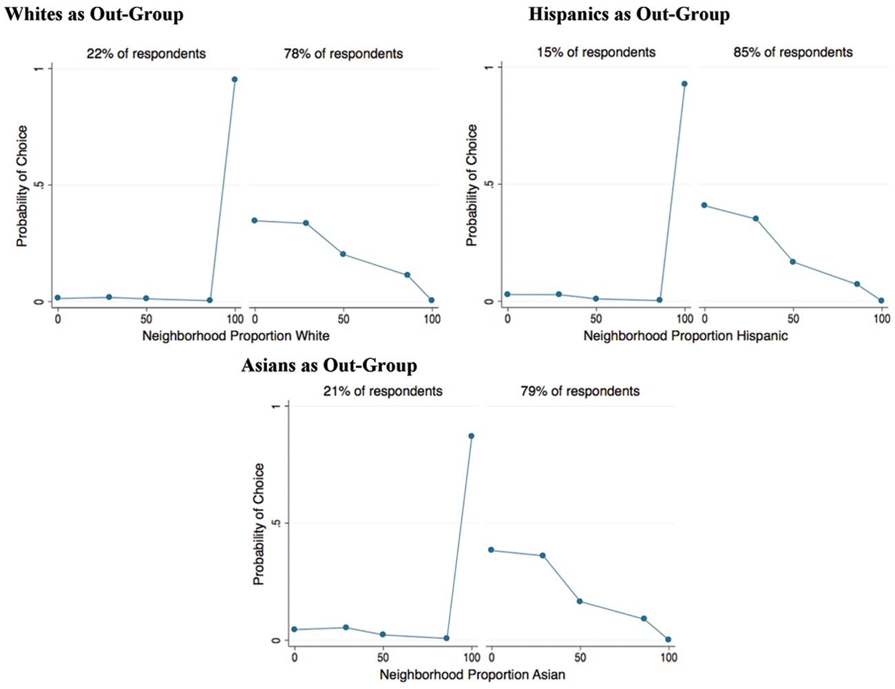
The results from estimating these models are shown for blacks and Hispanics in Figures 4 and 5, respectively. There is a clear pattern of response. For most respondents, the attractiveness of the neighborhood declines with the proportional representation of one’s own race/ethnic group. However, among Hispanic and black respondents who were asked about white neighbors, roughly one quarter indicate that the most attractive neighborhood is the one that is 100% white. Similarly, among blacks and Hispanics who were asked about living among Asians, 19% of Hispanics and 21% of blacks in the sample identify the all-Asian neighborhood as most attractive. These results are consistent with those reported by other analysts of the same data (e.g., Charles 2000).
Predicted probabilities for blacks, unmeasured heterogeneity models, 2 groups
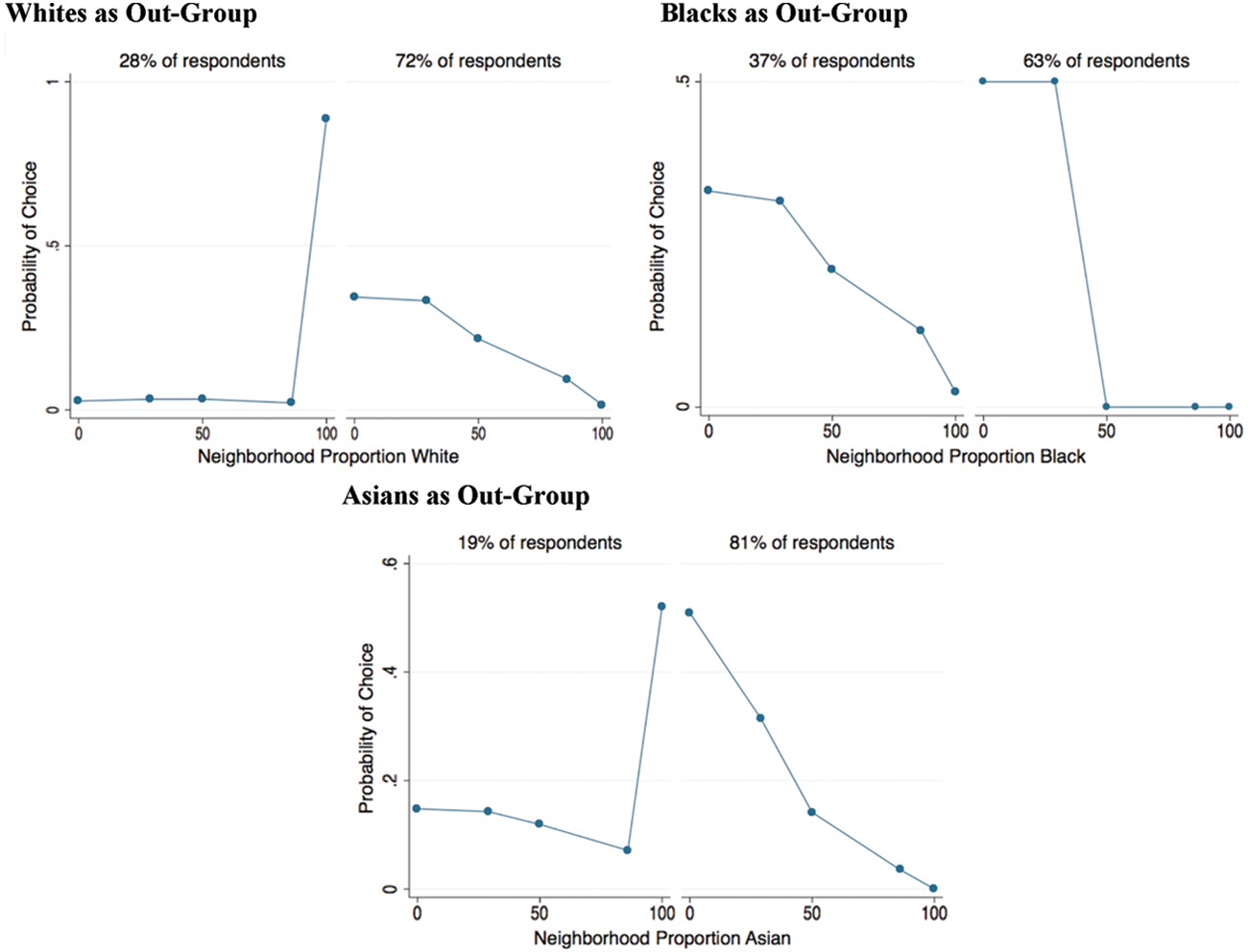
Predicted probabilities for Hispanics, unmeasured heterogeneity models.
7.2. Actual Mobility Histories in the LA FANS Data
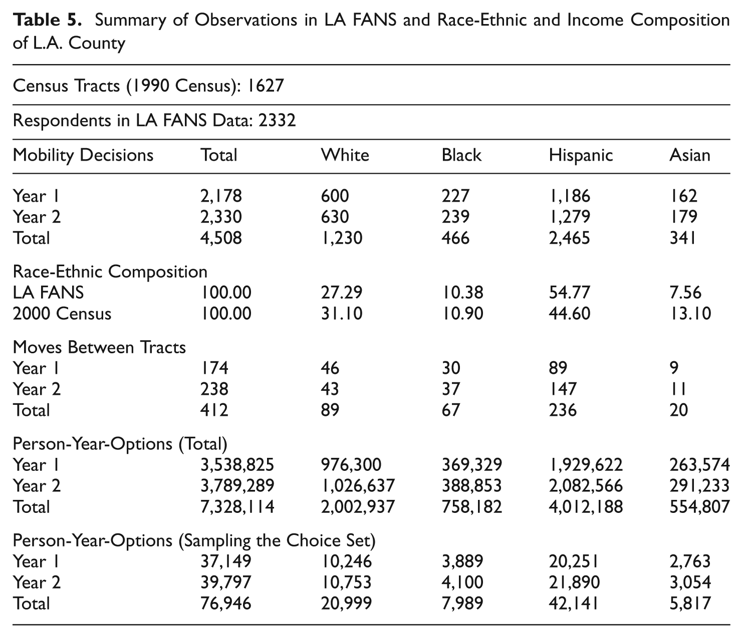
We illustrate how to analyze actual move data using the LA FANS Wave 1 data, which is a stratified sample of approximately 2,700 households in 65 Census tracts in Los Angeles County. The residential mobility history for each respondent was collected via an event history calendar for the 24 months preceding the survey date. Seventy percent of LA FANS respondents did not move during the two-year period prior to the interview, whereas 20% moved exactly once. Previous addresses in Los Angeles County are geolinked to the correspondent Census tract. However, we omit the small percentage (6.5%) of moves that occurred outside of Los Angeles County. We measure mobility in terms of annual moves, and observe up to two moves per respondent. Figure 6 shows one hypothetical mobility history for an LA FANS respondent. Because we examine annual mobility, multiple moves that occur within a single year are counted as a single move. Table 5 summarizes the information available for the analysis of residential mobility using the LA FANS data. 13 The 2,332 respondents provide information on 4,508 annual residential mobility decisions. 14 As indicated by the comparison with the 2000 Census data for Los Angeles County, our data overrepresent Hispanics and underrepresent non-Hispanic whites and Asians. Despite the relatively large number of mobility decisions faced by LA FANS respondents, they report only 412 annual between-tract moves during the two-year mobility window, and 105 within-tract moves. For the purposes of this analysis, we consider moves to occur only if a respondent changes Census tracts during the annual mobility period.
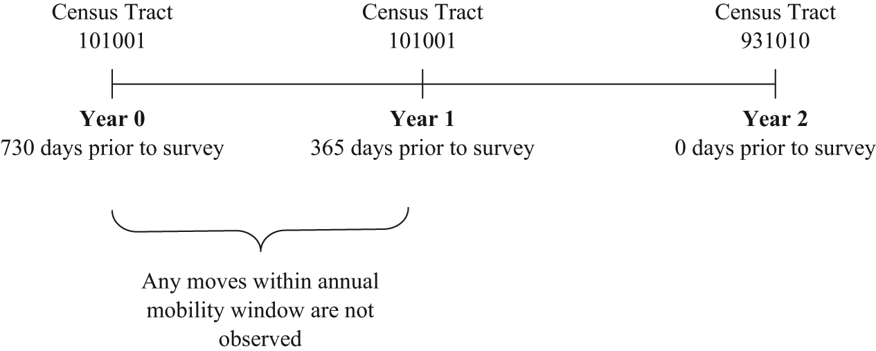
Example of one mobility history from the LA FANS.
Summary of Observations in LA FANS and Race-Ethnic and Income Composition of L.A. County
7.2.1. Choice-based Sampling
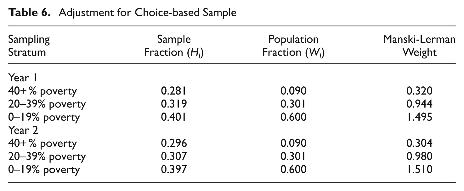
The LA FANS is a stratified sample that overrepresents neighborhoods where at least 40 percent of households have incomes below the poverty line. For the purpose of estimating models of neighborhood choice, LA FANS is a choice-based sample. Our models include Manski-Lerman weights (see Equation 16) to correct for the differential representation neighborhoods in the data. A further complication is that the data come from retrospective mobility histories. Thus, whereas LA FANS is a choice-based sample at the time of the survey, prior to that respondents could live anywhere conditional on living in one of the sampled tracts when the data were collected. Thus the sample is purely choice-based at the time of the survey (Year 2, as shown in Figure 6), but influenced in a complex way by the choice-based sample in the periods prior to the survey date. Thus, we create two sets of Manski-Lerman weights: one using the distribution of choices at the time the LA FANS sample was drawn (in Year 2 of the mobility window), and one using the distribution of choices one year prior (Year 1 of the mobility window).
Table 6 illustrates the construction of Manski-Lerman weights in the LA FANS. The first column (H i ) shows the distribution of respondents across the sampling stratum in each of the two years, whereas the second column (W i ) shows the distribution of the population across sampling stratum. The LA FANS overrepresents high-poverty neighborhoods in both years. The chosen neighborhoods of respondents were 28% high-poverty in Year 1 and 30% high-poverty in Year 2 (when the data were collected). In contrast, only 9% of Los Angeles County neighborhoods were high-poverty during this period. The sample distribution more accurately represents the population one year prior to the survey date because individuals could, in principle, live in any Los Angeles neighborhood during this period rather than only in one of the 65 sampled neighborhoods. The Manski-Lerman weights, which are the ratio of the population fractions to the sampled fractions in each stratum, are shown in column 3. The weights correct for over- and underrepresentativeness of sampled neighborhoods. The weights enter our discrete choice models using the “importance weights” option in Stata.
Adjustment for Choice-based Sample
7.2.2. Large Number of Choices
Table 5 shows the distribution of mobility decisions over years and race-ethnicity of respondents. The 1,627 occupied Census tracts in Los Angeles (based on the 1990 Census) are potential destinations in each of 4,508 sample mobility decisions, resulting in an effective sample size of 1,627 × 4,508 = 7,334,516 person-year options, far too many observations for a tractable analysis. Thus, we sample from the alternatives within each respondent’s choice set with probability 1.0 for chosen alternatives and 0.05 for unchosen alternatives. This produces the smaller number of person-year-options shown in the bottom panel of Table 5. The models include the correction factor,
7.2.3. Definition of the Choice Set and Aggregation of Choices
When people choose where to live, they select a specific housing unit within a neighborhood. However, our observations consist of moves within and between Census tracts, rather than actual dwelling units. Thus, we add a term to our models, In M j , where M j is the number of housing units in the jth Census tract, to take into account between-tract variation in the number of potential destinations. In measuring within-tract mobility opportunities this way, we assume that the fraction of dwelling units that are in fact available to the respondent is invariant across tracts. With more detailed data on housing vacancies, it may be possible to relax this assumption. We do not know the variation in housing desirability within each tract, and thus estimate a discrete choice model similar to Equation (14), but omitting the term B j .
7.2.4 Models of Residential Choice
We estimate conditional logit models that incorporate the effects of individuals’ personal characteristics and the characteristics of neighborhoods to which they might move, assuming that the choice set of each individual is all Census tracts in Los Angeles County. We allow for the possibility that respondents evaluate their current location differently from other potential destinations, by including a dummy variable Dij, which equals 1 when destination j is the neighborhood currently occupied by respondent i, and 0 otherwise. The model, which can be written as
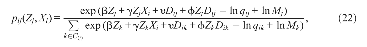
incorporates terms for sampling the choice set,
Effects of Respondent and Tract Characteristics on Residential Choice, LA FANS data
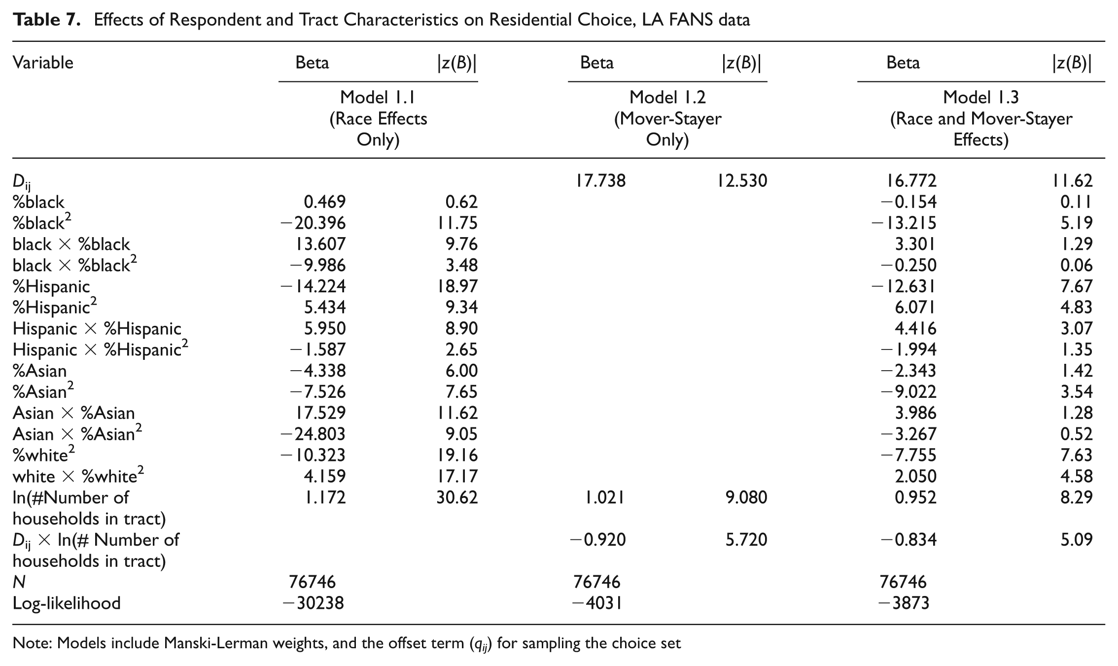
Note: Models include Manski-Lerman weights, and the offset term (qij ) for sampling the choice set
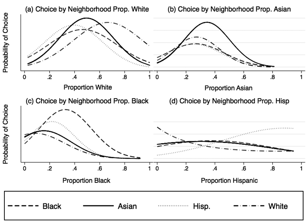
Predicted probabilities for whites, blacks, Asians, and Hispanics, LA FANS movers, by ethnic proportions
8. Linking Residential Mobility Decisions to Neighborhood Change
Residential choice models predict the probabilities that individuals with varying characteristics select a neighborhood or housing unit, conditional on features of that alternative and of other potential destinations. Taken alone, these probabilities are ambiguous in their implications for aggregate neighborhood change because the choice probabilities estimated from these models describe the behavior of the marginal individual rather than the expected flows of population subgroups. At the aggregate level it is necessary to recognize that the mobility behaviors of all individuals are interdependent; that is, individuals respond to the composition of their local areas and all potential destinations, but their responses change that composition. When behavior is interdependent, there is feedback from the aggregate to the individual level and no simple relationship between the choices of individuals and the residential patterns that result. To understand the implications of residential choice for neighborhood change, we need to connect individual-level probabilities with the distribution and size of the relevant population groups. We discuss three strategies for making this connection: (1) interactive Markov models, (2) general equilibrium models with price effects, and (3) agent-based models. Each method allows residential choice to change the attributes of neighborhoods, which affects subsequent mobility decisions. Markov and general equilibrium models are variants of macrosimulation approaches, representing mobility as expected rates of transition among neighborhoods or aggregate market adjustments respectively, whereas agent based models are microsimulations, in which individual mobility decisions are realizations of probabilistic choice. 15 Markov and agent-based models are dynamic models that are useful for estimating the changes in population distribution across neighborhoods that result from underlying regimes of individual residential preferences. These changes can be pathways to an equilibrium residential distribution or between nonequilibrium states. General equilibrium models are useful for exploring the variation in equilibrium population distributions across neighborhoods associated with variation in exogenous conditions.
All three approaches assume a population of individuals distributed across a neighborhood environment and a set of rules governing mobility behavior. Individuals may be drawn from a hypothetical or a realistic population. An example of a hypothetical population involves two groups, each constituting 50% of the population, whereas a realistic population may be specified by Census data—for example, all households in Los Angeles County. The environment may be a highly stylized landscape (such as a 10 by 10 grid, where each cell on the grid represents a potential destination) or a realistic city (such as all Census tracts in Los Angeles County). The key features of the landscape are characteristics endogenous to the mobility process, such as neighborhood race-ethnic and economic composition. Fixed features, such as elevation, the location of highways and commercial areas, and air quality, may also be included. However, only neighborhood characteristics that can be represented as aggregates of individual characteristics and that affect individual decisions have a dynamic component. Neighborhood boundaries may be objectively defined, as in the case of Census tracts where all inhabitants of the same tract have the same neighborhood boundaries. Alternatively, in the case of agent-based models, neighborhoods can be defined such that each household has its own unique neighborhood. In all cases, individuals have rules for evaluating neighborhoods. In the cases we discuss below, this rule is operationalized through a discrete choice model. In all these models, the composition of neighborhoods is an endogenous outcome of the model. Each move between times t and t + 1 changes the opportunity structure for all individuals who contemplate a move between t + 1 and t + 2. Thus, all models incorporate not only the aggregate implications of individual preferences but also the feedback effects of aggregate change on the mobility behavior of individuals.
8.1. Interactive Markov Models
Markov models link a set of individual- or group-specific residential mobility probabilities to expected patterns of neighborhood turnover. A Markov model has a finite set of J states,

where superscript

This is equivalent to the operation of summing over transition probabilities within destinations

where

Here m[t] represents the distribution of blacks and whites across neighborhoods, and the probability of moving into a given neighborhood is a function of its ethnic composition. In this model, preferences for neighborhood characteristics are fixed, but the attractiveness of specific neighborhoods changes as a result of their changing characteristics.
To illustrate the interactive Markov model, we consider a simple city with two neighborhoods and a population of 10 blacks and 10 whites. At time 0 the population is completely segregated; all blacks are in one state, and all whites are in the other. Next, we compute the population trajectory for whites and blacks using their respective preference functions. For example, if people evaluate their neighborhoods according to a simplified version of Equation (4), where the probability that the ith person selects the jth neighborhood is
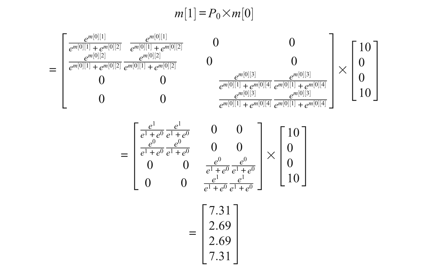
At step 2,
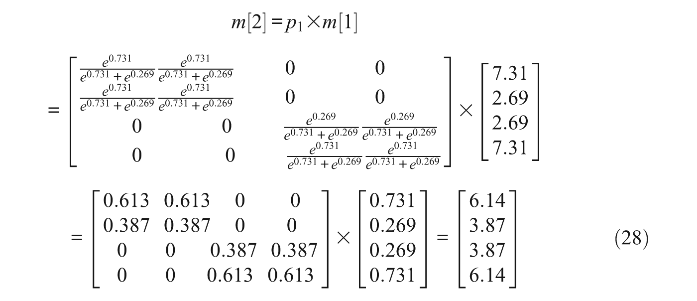
The process can continue until the neighborhoods reach equilibrium—that is, where Π
8.2. General Equilibrium Models with Price Effects
Another strategy for studying neighborhood dynamics is using general equilibrium (GE) models with price effects. Bayer and colleagues (Bayer and McMillan 2008; Bayer, McMillan, and Rueben 2004) use GE models to examine the relationship between residential choice behavior and neighborhood outcomes. The analysis consists of two parts: (1) estimating a discrete choice model and (2) simulating the expected distribution of individuals in each neighborhood implied by the choice model. GE models assume that observed neighborhoods are in equilibrium, such that each individual had made an optimal choice given the choices of all other individuals. The models can be used to show how a new equilibrium distribution of neighborhoods results from some change in initial conditions or behavior (e.g., assuming that people are indifferent to the racial composition of their neighborhoods or assigning all ethnic groups equal income distributions). The first step is assuming or estimating a discrete choice model for the effects of housing prices, neighborhood race-ethnic composition, and other factors (as discussed in Section 6). Given this model, it is possible to simulate the impact of counterfactual conditions. For example, choice-model coefficients associated with neighborhood race-ethnic composition may be set to zero, to represent a city in which people make race-blind residential decisions and, using this modified choice model, it is possible to compute a new equilibrium distribution of neighborhoods.
In the first stage, predicted probabilities are computed representing the likelihood that an individual with a given demographic profile chooses a neighborhood of a given demographic composition. These probabilities are summed over neighborhoods to generate the demographic composition of neighborhoods in the next time period. Residential choice probabilities are recomputed to take into account changing neighborhoods, and the procedure repeats. More formally, the demographic composition of neighborhoods at time

where s
j
and
8.3. Agent-based Models
Agent-based models are a third approach to linking individual mobility to neighborhood dynamics (Macy and Willer 2002; Bonabeau 2002). Such models are microsimulations in which hypothetical individuals make choices based on either assumed behavioral rules or a statistical model of behavior. Agent-based models explicitly represent the feedback between individuals’ behavior and aggregate processes (e.g., residential mobility and neighborhood change, mate preferences and marriage market dynamics, decisions to smoke or drink and high school norms around these behavior), and they can allow for detailed geography and individual heterogeneity. Schelling’s (1971, 2006) model of residential tipping is an example of an agent-based model of a social process. Related models have been used to study norms regarding age at first marriage (Todd, Billari, and Simao 2005), income inequality and racial residential segregation (Bruch 2011), and other phenomena.
Agent-based models contain a population of actors who are assigned behaviors appropriate to the substantive application. An agent-based model of residential mobility assumes rules about how agents evaluate the desirability of neighborhoods and decide when and where to move. These rules can be simple heuristics or a more complex model such as that provided by the coefficients of a discrete choice model. If agents’ behavior is grounded in a discrete choice model, they use the values of neighborhood characteristics in their simulated world (as well as their own attributes) in combination with the model parameters to generate transition probabilities for moving among neighborhoods. The agent translates these transition probabilities into a (multinomial) distribution for the probabilities of selecting each neighborhood and “samples” a neighborhood via a draw from this distribution. In practice, the neighborhood-specific probabilities are cumulated, and the agent picks a neighborhood by drawing a number between 0 and 1 and choosing the neighborhood associated with the interval that contains that number. Figure 8 illustrates this process. See Bruch and Mare (2006, 2009) for a more detailed description of how to incorporate discrete choice models of residential mobility into agent-based models of neighborhood dynamics.
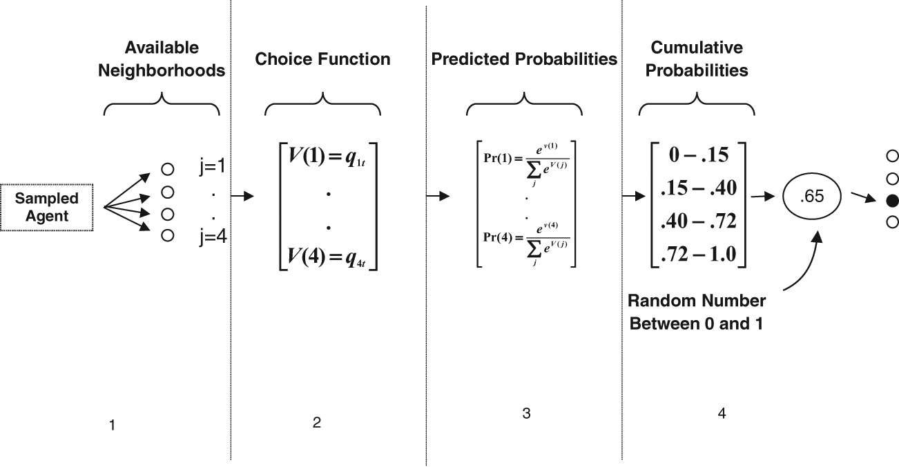
Determining chosen destination for agent using discrete choice framework.
There are a number of software packages available for doing agent-based modeling, including Mason, Swarn, and Ascape. Netlogo (http://ccl.northwestern.edu/netlogo/) and Repast (http://repast.sourceforge.net/) are two of the most widely used options; both are free. Netlogo is a good option for researchers new to object-oriented programming. It is aimed at a less technical audience, has extensive documentation and user support, and contains a number of basic social science models in its model library. Repast requires some knowledge of Java, but can be used to run more complex models with larger populations. The software also allows for parallel processing. Both programs allow the user to import Geographic Information Systems (GIS) data to simulate mobility using realistic geography.
8.4. Comparing Approaches for Micro and Macro Linkage
Each of the three approaches takes a different tack to looking at segregation processes. Both Interactive Markov (IM) models and General Equilibrium (GE) models focus on the aggregate distributions of populations across neighborhoods, whether estimated in practice from aggregate or individual-level data. As they have been applied to residential choice studies, however, GE models are used for comparing equilibria under alternate assumptions, whereas IM models are used to examine the dynamics of residential mobility and neighborhood change (contrast Mare and Bruch 2003 using IM models with papers by Bayer and colleagues). Like interactive Markov models, agent-based models also focus on population dynamics, but they are built up from the actions of simulated individuals. However, there are two key differences between agent-based models and the GE and IM models: (1) Agent-based models have an explicit notion of “vacancies,” where agents can move into an area only if there is an available slot; and (2) individuals in agent-based models make realized—not probabilistic—decisions. These differences may lead to substantively different segregation dynamics (for the same population and behavioral model).
9. Future Directions in Residential Mobility Research
There are several promising directions for future research into residential mobility patterns and neighborhood change. One is the development of two-sided matching models for the coordination of housing seekers with housing providers. In the discrete choice models discussed in this paper, we treat the choice to move into a unit separate from the choice of the previous occupant to move out of a unit, without explicitly representing housing vacancies, whether transitory or longer term. We can imagine viewing the flow of people in and out of housing units as a coordinated set of simultaneous moves. This may be more analogous to real-world mobility behavior in that most housing units are not vacant for long periods of time, as residents move out and then in again in a matter of hours or days. The use of data on moves, housing stock (including vacancies), housing searches, prices, and real estate transactions would greatly enhance knowledge on residential mobility and neighborhood change.
A second research direction involves finding better tools for aggregate model evaluation. Agent-based models, interactive Markov models, and general equilibrium models are all tools for linking residential mobility behavior described by discrete choice models with aggregate patterns of neighborhood change. However, further work is needed to develop tools for evaluating the inferences from these models from sample or fragmentary population data (Berk 2008).
Despite their limitations, the discrete-choice modeling approach can reveal a great deal about how people choose where to live and the implications of these choice patterns for neighborhood change. The techniques discussed in this paper also potentially have relevance for a wider range of applications, including choice of marriage partner and aggregate patterns of assortative mating, the choice of occupation or academic field and the aggregate composition of the people holding that occupation or degree (e.g., England et al. 2007), and the choice of friends in high school and the composition of peer networks.
Footnotes
Appendix. MCSUI Residential Preference Questions
Acknowledgements
The paper benefited greatly from the comments provided by three anonymous reviewers.
Declaration of Conflicting Interests
The authors declared no potential conflicts of interest with respect to the research, authorship, and/or publication of this article.
Funding
The authors disclosed receipt of the following financial support for the research, authorship, and/or publication of this article: The authors acknowledge funding from the Robert Wood Johnson Foundation, the National Science Foundation, and the John D. and Catherine T. MacArthur Foundation.