
Abstract
To understand how income inequality affects individuals and communities, researchers must have accurate measures of income inequality at lower geographic levels, such as counties, school districts, and census tracts. Studies of income inequality, however, are constrained by the tabular format in which censuses publish income data. In this article, the author proposes a new method, Lorenz interpolation, for estimating income inequality from binned income data. Using public microsample data from the American Community Survey (ACS), the author shows that Lorenz interpolation produces more accurate and reliable income inequality estimates than do alternative estimation methods. Then, using restricted ACS income data obtained through a Federal Statistical Research Data Center, the author evaluates the accuracy of Lorenz interpolation at the census tract and school district levels. Lorenz interpolation produces reliable school district–level estimates, but the method produces less reliable estimates for some income inequality measures at the tract level. These findings indicate that researchers should refrain from estimating tract-level income inequality measures from tabular data. They also show that aggregating tract income distributions to higher geographic levels can produce valid estimates of income inequality.
Income inequality has increased substantially in many countries around the world. In the United States, income inequality is higher today than it has been at any point since the beginning of the Great Depression (Galster and Sharkey 2017). Rising income inequality has been implicated in a range of negative public health consequences (Pickett et al. 2005; Pickett and Wilkinson 2007), and research shows a connection between income inequality and economic segregation (Reardon and Bischoff 2011), which has implications for educational stratification (Owens 2016). Growing income inequality has also driven increasing inequities in the intergenerational transmission of wealth (Chetty et al. 2017), which has led to decreased levels of social mobility (Grusky and MacLean 2016).
Amid growing concern around these and other possible consequences of rising income inequality, researchers have sought ways to measure the distribution of income more precisely to trace how and where it is changing over time. They are constrained in their efforts, however, by the format in which most countries release their income data. To protect respondent confidentiality, censuses generally publish income data in tabular format, as counts in income brackets ($0–$9,999, $10,000–$14,999, . . ., ≥$200,000). Researchers attempting to use these data to estimate income inequality must make assumptions about how incomes are distributed within these brackets. Moreover, the highest income bracket in these data is always unbounded at the top, which makes estimating the upper tail of the income distribution especially difficult. For some income inequality measures, even small errors in estimation of this upper tail can lead to large errors in estimation of income inequality.
A number of studies have proposed methods to estimate income statistics using grouped income data (Gastwirth and Glauberman 1976; Hajargasht et al. 2012; Jargowsky and Wheeler 2018; Kakwani 1976; Minoiu and Reddy 2012; Quandt 1966; Tillé and Langel 2012; von Hippel, Hunter, and Drown 2017; von Hippel, Scarpino, and Holas 2016). Two recent studies show that income distribution means, which are provided in the public portions of many national censuses, can be used to produce more accurate estimates of income inequality (Jargowsky and Wheeler 2018; von Hippel et al. 2017). Still, two problems remain. First, even these methods have difficulty with inequality measures that rely heavily on the upper tail of the income distribution. This is unfortunate because some of these measures have desirable properties. For instance, the Theil coefficient can be decomposed into groups to determine how different kinds of households or people contribute to income inequality. This makes Theil coefficients useful to researchers interested in understanding how changing levels of income inequality between geographic subregions or racial groups have contributed to overall changes in income inequality.
Second, these methods have been evaluated only using income data for large geographic regions, such as metropolitan areas and counties. To understand the social consequences of income inequality, it often makes more sense to focus on a lower geographic level. For instance, someone interested in the relationship between income inequality and educational inequality may want to work at the level of the school district, which determines the portion of a school’s budget that comes from property taxes, or the school attendance zone, which delineates which schools a child is eligible to attend. Alternatively, if a researcher wants to understand how income inequality is experienced in one’s community, the relevant geography might be the neighborhood, which is often operationalized by census tract. Given that geographies such as these cover areas with smaller populations, existing methods for estimating income inequality may be insufficiently reliable when deployed at lower levels of analysis. Some researchers have admonished against using these methods to estimate inequality for smaller geographic regions (von Hippel et al. 2016), but how these methods fare at producing income inequality estimates for these regions has yet to be empirically tested.
In this article, I outline a new method for estimating income inequality from grouped income data. The method, which I call Lorenz interpolation, consists of using income quantiles derived from these data to estimate the Lorenz curve of the underlying income distribution. 1 This Lorenz curve is used to create a weighted sample of exact incomes, from which income statistics can be derived. A key advantage of Lorenz interpolation over other methods comes from the accuracy with which the method estimates the upper tail of the income distribution. 2
Using public microsample data from the 2011 to 2015 American Community Survey (ACS) and working at the public-use microdata area (PUMA) level, I show that Lorenz interpolation outperforms mean-constrained integration over brackets (MCIB) and cumulative density function (CDF) interpolation at estimating income inequality, especially inequality measures that are sensitive to the upper tail of the income distribution. Then, I evaluate the performance of Lorenz interpolation at two lower geographic levels, the census tract level and the school district level, using restricted census data to which I have been granted access through a Federal Statistical Research Data Center (FSRDC). 3 Results indicate that Lorenz interpolation produces more accurate estimates of income inequality at all three geographic levels. However, tract-level estimates are insufficiently reliable for most analyses. Lorenz interpolation yields more accurate estimates of the Gini, Theil, and Atkinson coefficients at the school district level. Geographies such as these that consist of small groups of census tracts are sufficiently large for the accurate estimation of income inequality. I conclude with a discussion of the use cases of Lorenz interpolation and some unresolved issues surrounding the measurement of income inequality.
Background
A common method for deriving income inequality statistics from grouped income data is to set the incomes in the closed income bins to their midpoints and estimate a Pareto distribution for the open bin at the top of the income distribution (Henson 1967; Jargowsky 1996).
4
Fitting a Pareto distribution to the top bin requires that one estimate a Pareto distribution shape parameter,

where
One problem with this method is that mean estimates of the top bin derived from the Pareto-linear procedure are not robust to even small errors in estimation of
Recently, researchers have gotten around limitations of the midpoint-Pareto imputation method by using the income distribution mean to estimate probability and CDFs from grouped income data. 5 Proposing a method called CDF interpolation, von Hippel et al. (2017) use grouped income data to plot a set of points along the CDF of the income distribution. After interpolating the CDF, the authors drew from the income distribution mean to apply an upper bound to the CDF. 6 Income statistics are derived from the CDF through numerical integration. When tested on county-level income distributions, the authors showed that CDF interpolation estimates Gini coefficients within 1 percent to 2 percent of their true values (von Hippel et al. 2017:651). 7
Jargowsky and Wheeler (2018) also proposed a method that takes advantage of the income distribution mean. Rather than fitting a function to points along the CDF, the authors estimated a probability density function (PDF) directly from the grouped income data. Their technique, which they called mean-constrained integration over brackets, consists of estimating a piecewise linear function for the closed income bins, fitting a Pareto distribution to the top bin, and integrating over the resulting distribution. 8 MCIB uses the mean of the income distribution to estimate the mean of the top income bin. 9 The authors showed their method outperforms many estimation techniques that do not incorporate the income distribution mean.
Methods that use the income distribution mean produce more accurate estimates of some inequality measures, but these techniques are less successful at estimating parameters that are sensitive to the upper tail of the income distribution. This is because the top bin in grouped income data usually does not have an upper bound. The method I put forth here provides more accurate estimates of inequality measures that rely on the upper tail of the income distribution. This method, which I call Lorenz interpolation, uses the income quantiles contained in grouped income data to estimate a Lorenz curve.
Lorenz curves visually represent the level of inequality in a distribution. To create a Lorenz curve from a set of incomes, one sorts these incomes in ascending order and computes a running sum. This is divided by the total income to produce a cumulative income share, which is plotted against the cumulative population share. The cumulative population share is plotted on the x axis, and the cumulative income share is plotted on the y axis.
Much of the information about the shape of the Lorenz curve is provided by the income quantiles in grouped income data. The connection between income quantiles and the Lorenz curve is reflected by the following equation 10 :

where
Although Lorenz curves are rarely found in sociological research, economists have developed techniques to estimate inequality statistics by interpolating the Lorenz curve (Cowell and Mehta 1982; Gastwirth 1971; Gastwirth and Glauberman 1976; Gastwirth, Nayak, and Krieger 1986; Tillé and Langel 2012). Many of these techniques were developed for data that contain more information about the income distribution than do the data in many national censuses (e.g., Cowell and Mehta 1982). In contrast, this study imposes the same limitations on the data as those found in publicly available income data.
Methods
Lorenz interpolation produces income statistics by building a spline function that approximates the Lorenz curve of the underlying income distribution. Each segment of this spline is a cubic function estimated using points on the Lorenz curve and a set of constraints that determine slopes for the Lorenz curve at each of the income boundaries. The estimated Lorenz curve is used to produce a weighted sample of exact incomes, from which inequality statistics are derived.
Building a Lorenz Curve from Grouped Income Data
Figure 1 illustrates the steps though which Lorenz interpolation estimates a Lorenz curve. The vertical dashed lines represent cumulative population shares that can be computed from the grouped income data. The income boundaries associated with these lines are used to compute slopes along the Lorenz curve, which are represented by the gray line segments.
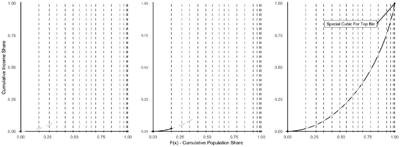
Lorenz interpolation in three steps.
Lorenz interpolation approximates a Lorenz curve by estimating several cubic functions in a sequence. The left plot of Figure 1 shows the first cubic defined by Lorenz interpolation. This function is constrained to pass through (0, 0), the point at which the Lorenz curve begins. The slope of the function is constrained to equal
The absence of an upper bound makes defining a cubic function for the top bin particularly challenging. Cubic functions fit to points along the Lorenz curve potentially underestimate the variance of incomes at the top of the income distribution (Kakwani 1976:489). To remedy this issue, Lorenz interpolation uses slope constraints to control the rate at which the cubic function applied to this bin curves upward. First, a quadratic function is defined that passes through two points, (
Having estimated a Lorenz curve, the final step is to create a sample of exact incomes based on this curve. A computationally efficient way to do this is to plot equidistant points along the Lorenz curve and multiply the slopes of the line segments connecting these points by the income distribution mean. This generates samples from the underlying income distribution, which can be weighted using the frequencies in the grouped income data. This weighted sample is used to produce various income statistics.
The PDF Implied by Lorenz Interpolation
The PDF implied by Lorenz interpolation is a piecewise function consisting of several square root functions. This can be recognized by deriving the PDF from the Lorenz curve. Equation (3) shows a segment of the estimated Lorenz curve,

where
To compute the PDF from the Lorenz function, one must first derive the CDF from this function. One way to do this is to use the following rule noted by Gastwirth (1971):

This is the definition of the Lorenz curve as a function of the cumulative population share

It follows that taking the derivative with respect to

Everything can be moved to the right side of the equation by dividing both sides by

The function for the CDF,
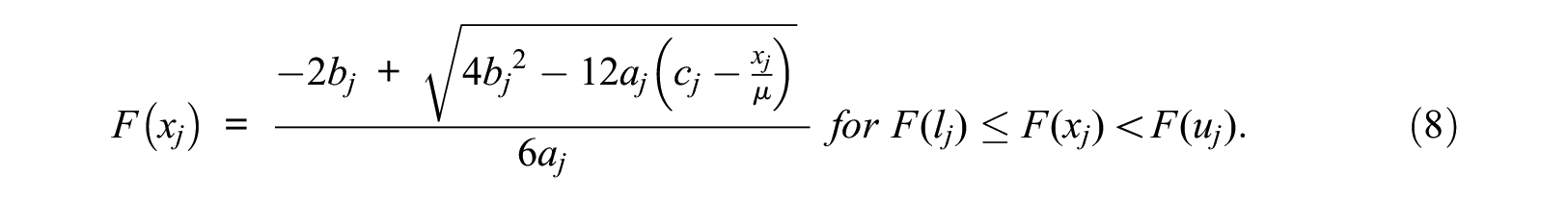
Taking the derivative of both sides with respect to
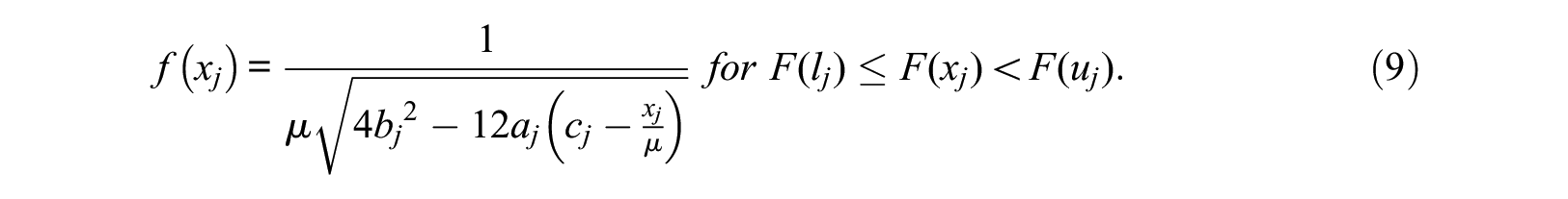
Finally, the domain is rewritten in terms of

Note that the slope constraints used to compute
Figure 2 shows an example of a PDF based on Lorenz interpolation. The spikes along the upper tail of the income distribution are a result of the square root function Lorenz interpolation uses to approximate each bin of the income distribution. These spikes indicate some clustering of incomes at the bin lower bounds along the upper tail of the income distribution. Despite the presence of these spikes, the results show that Lorenz interpolation yields accurate estimates of local income statistics such as bin means, income quantiles, and income shares.
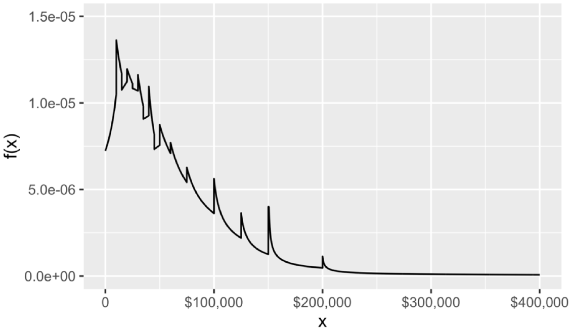
Example of a probability density function based on Lorenz interpolation.
Data and Measures
Data for this study come from the 2011 to 2015 five-year pooled ACS. The ACS contains social and economic data for the U.S. population and is administered on a rolling basis by the U.S. Census Bureau. To provide more reliable estimates, the Census Bureau publishes ACS data in five-year groupings, which cover roughly 5 percent of the U.S. population (Ruggles et al. 2021). I used household income data from the public-use microdata sample (PUMS) component of the ACS, which contains households’ exact incomes. 14 I calculated estimates of income inequality for 1,185 PUMAs, which are the smallest geographies for which PUMS data are available.
To calculate income inequality for tracts, I used restricted census data to which I was granted access through a FSRDC. These data contain exact incomes with geographic information down to the block level. To produce income inequality estimates for school districts, I used a crosswalk between census tracts and school districts from the National Center for Education Statistics (Geverdt 2019). Tract-level incomes were assigned to school districts on the basis of the distribution of each tract’s land area across school districts. For example, if 60 percent of a tract’s area is in district A and 40 percent is in district B, 60 percent of its incomes were assigned to district A and the remaining 40 percent were assigned to district B. School-district data are based on boundaries from 2013, which falls in the middle of the study period (2011–2015). These analyses were based on 69,675 tracts and 13,360 school districts.
Evaluating Lorenz Interpolation
To assess the performance of Lorenz interpolation, I created two data sets, an exact income data set and a grouped income data set. The latter was produced by converting each region’s exact income data into counts in income brackets, which were determined by the income bounds the Census Bureau has used since 2000. I calculated each region’s “true” level of income inequality by plugging the exact income data into an income inequality formula. 15 I applied Lorenz interpolation to the grouped income data to generate an income inequality estimate. Finally, I calculated the error metrics by comparing “true” and estimated income inequality.
I evaluated Lorenz interpolation with four measures of income inequality. First, I looked at Gini coefficients, which can be computed using the following formula:

The Gini coefficient is the mean absolute difference among incomes divided by twice the aggregate income. Next, I computed the Theil coefficient. Based on information theory, Theil coefficients account for the level of entropy, or unpredictability, in a data set. Income distributions with low entropy have higher Theil coefficients, which indicate more inequality. Theil coefficients are calculated using the following formula:

One nice feature of Theil coefficients is that they can be decomposed to determine contributions from different groups. This means that Theil contributions can be estimated for each bin of an income distribution. Performing such a decomposition shows that most of the Theil coefficient can often be attributed to the top bracket of grouped income data. I also computed the Atkinson index (Atkinson 1970). This measure includes a parameter that determines the relative influence of the lower and upper tails of the income distribution. It is defined by the following equation:
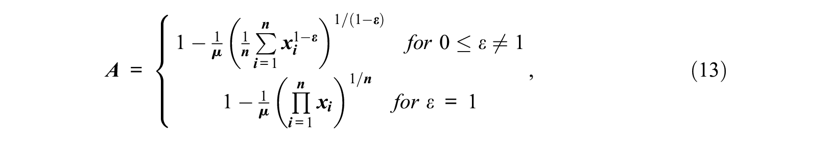
where
I compared the numbers generated from Lorenz interpolation to estimates from two other methods: von Hippel et al.’s (2017) CDF interpolation method and Jargowsky and Wheeler’s (2018) MCIB method. To implement CDF interpolation, I used the binsmooth package in R (Hunter and Drown 2016). To implement MCIB, I used Jargowsky’s (2019) MCIB module, which is available in Stata.
Results
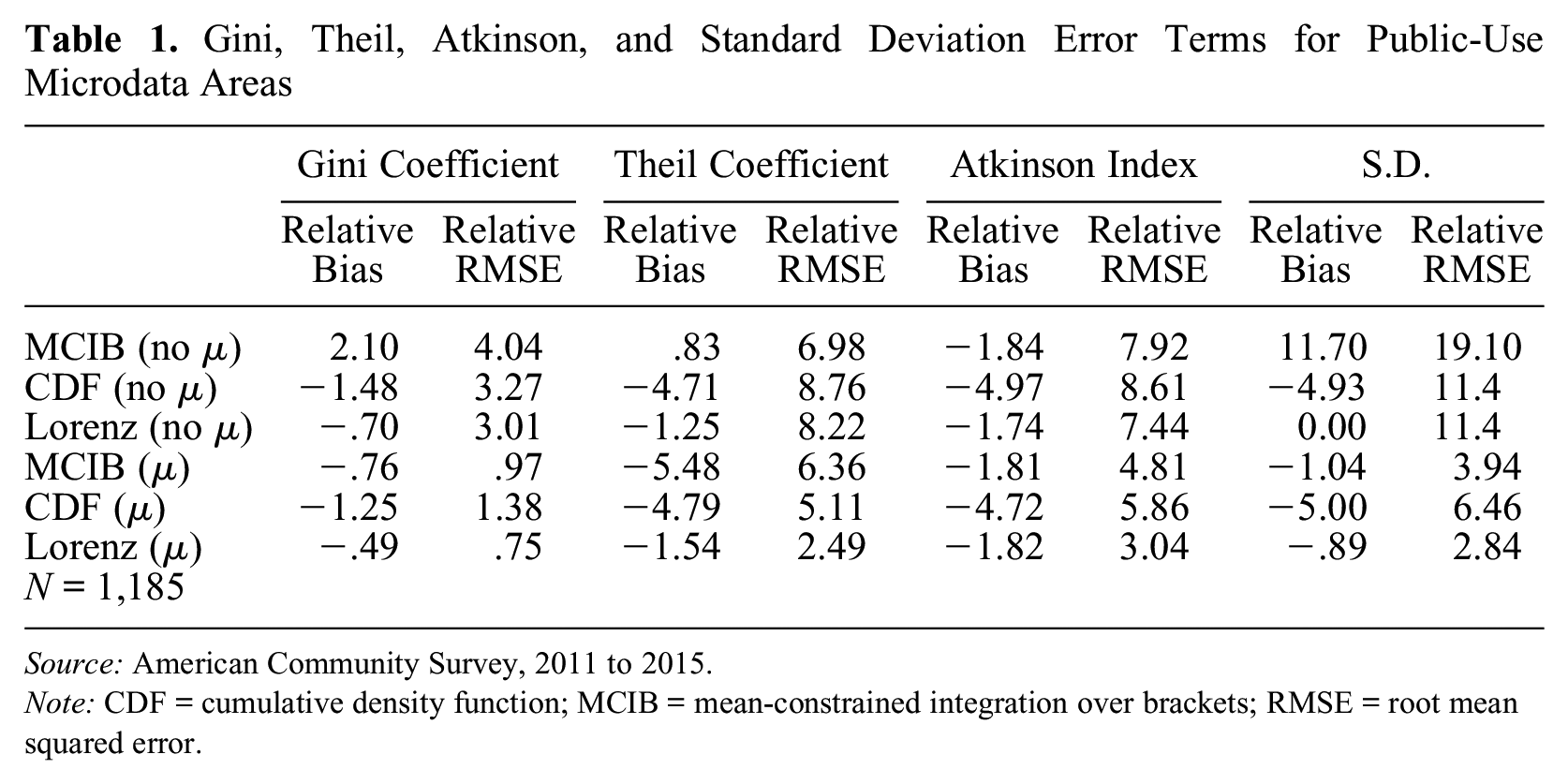
Table 1 compares error terms from Gini, Theil, Atkinson, and standard deviation estimates based on MCIB, CDF interpolation, and Lorenz interpolation. The top three rows show the errors produced by running these methods without the income distribution means, and the bottom three rows display errors based on estimates that incorporate the income distribution means.
16
Following von Hippel and colleagues (2017), I calculated the percentage relative bias and percentage relative root mean squared error (RMSE) of the estimates. These measures are based on the percentage estimation error (
Gini, Theil, Atkinson, and Standard Deviation Error Terms for Public-Use Microdata Areas
Source: American Community Survey, 2011 to 2015.
Note: CDF = cumulative density function; MCIB = mean-constrained integration over brackets; RMSE = root mean squared error.
Looking at the first three rows of the table, which compare inequality estimates without the income distribution mean, CDF interpolation outperformed MCIB at estimating the Gini coefficient and the standard deviation, and MCIB outperformed CDF interpolation at estimating the Theil and the Atkinson coefficients. Lorenz interpolation outperformed both methods at estimating the Gini coefficient, Atkinson coefficient, and standard deviation, and it performed worse than MCIB at estimating the Theil coefficient. Turning to estimates that incorporate the income distribution mean, Lorenz interpolation estimates had lower relative RMSEs for all four inequality measures and lower relative bias for all measures except the Atkinson coefficient. For Theil coefficients, Atkinson measures, and standard deviations, Lorenz interpolation produced considerably more accurate estimates as measured by the relative RMSE. Whereas Theil coefficient estimates based on MCIB had a relative RMSE of 6.36 percent, Theil coefficients from Lorenz interpolation had a relative RMSE of 2.49 percent. Furthermore, standard deviation estimates based on CDF interpolation had a relative RMSE of 6.46 percent, whereas standard deviation estimates from Lorenz interpolation had a relative RMSE of only 2.84 percent. Although Lorenz interpolation also outperformed the other methods at estimating the Gini coefficient, all three methods produced highly accurate Gini coefficient estimates, with relative RMSEs ranging from 0.75 percent to 1.38 percent.
Table 2 compares the relative bias and RMSE terms of bin mean estimates based on MCIB, CDF interpolation, and Lorenz interpolation. This table also includes the error terms for each method’s estimate of the total closed bin income, which determines the top bin mean estimates.
Bin Mean Error Terms for Public-Use Microdata Areas
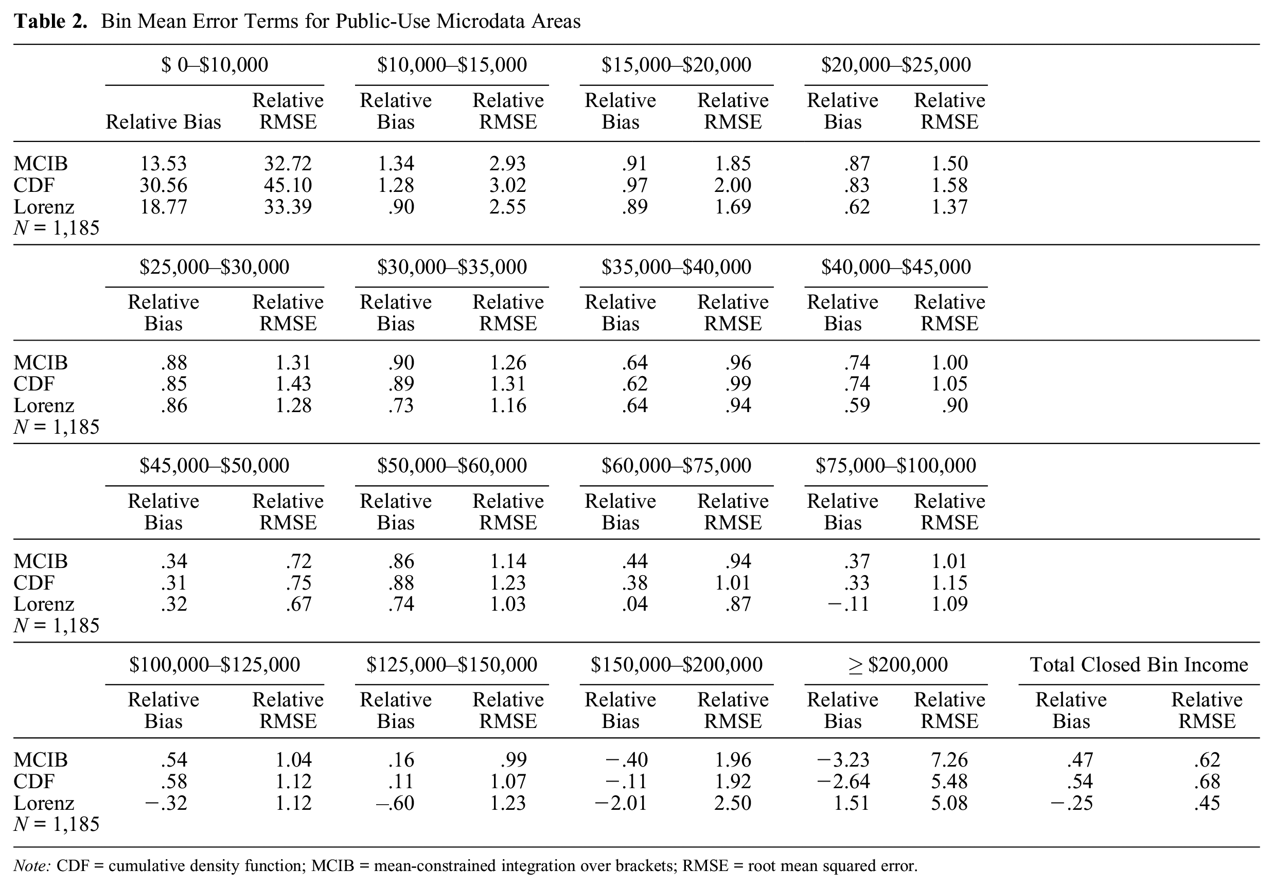
Note: CDF = cumulative density function; MCIB = mean-constrained integration over brackets; RMSE = root mean squared error.
Among the 16 bin mean estimates shown in Table 2, MCIB had the lowest relative bias for 1 bin and the lowest relative RMSE for 4 bins, CDF interpolation had the lowest relative bias for 5 bins and the lowest RMSE for 1 bin, and Lorenz interpolation had the lowest relative bias for 10 bins and the lowest relative RMSE for 11 bins. Lorenz interpolation also had the lowest relative bias and RMSE for the total closed bin income. Both MCIB and CDF interpolation produced positively biased estimates of the total closed bin income. As a result, these methods produced negatively biased estimates of the top bin mean.
The greater accuracy of Lorenz interpolation can be attributed in part to how this method estimates the top bin mean, but this does not tell the whole story. Although Atkinson index estimates based on Lorenz interpolation had slightly higher relative bias than MCIB Atkinson index estimates, the relative RMSE of MCIB Atkinson index estimates was significantly higher. This reflects the latter method’s use of the Pareto distribution to approximate the upper tail of the income distribution. Figure 3 shows scatterplots for the residuals of Atkinson index estimates from all three estimation methods. The solid lines denote the bias associated with each estimation method, and the dashed lines represent a 1 standard deviation distance from the solid lines. Comparing the space between the dashed lines in each plot, Lorenz interpolation had more reliable estimates than those produced using the other methods. The difference in reliability of Lorenz interpolation estimates is even larger at the school district and census tract levels.
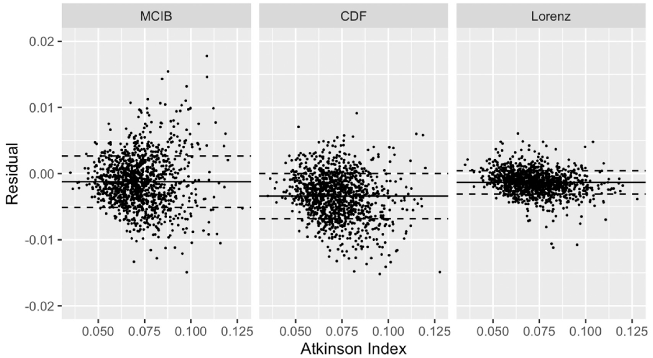
Residuals from Atkinson estimates.
Estimating Tract-Level and School District–Level Inequality Measures
Estimates of income inequality based on grouped data are less accurate for small regions (von Hippel et al. 2016). This is due chiefly to sampling variation, but it may also reflect the heterogeneity of income distributions associated with smaller regions. The income distributions of neighborhoods or municipalities vary more than those of larger regions such as metropolitan areas, which encompass entire regional economies and may resemble each other more. This raises the question of whether estimation techniques such as Lorenz interpolation can be used to produce valid income inequality estimates for small areas.
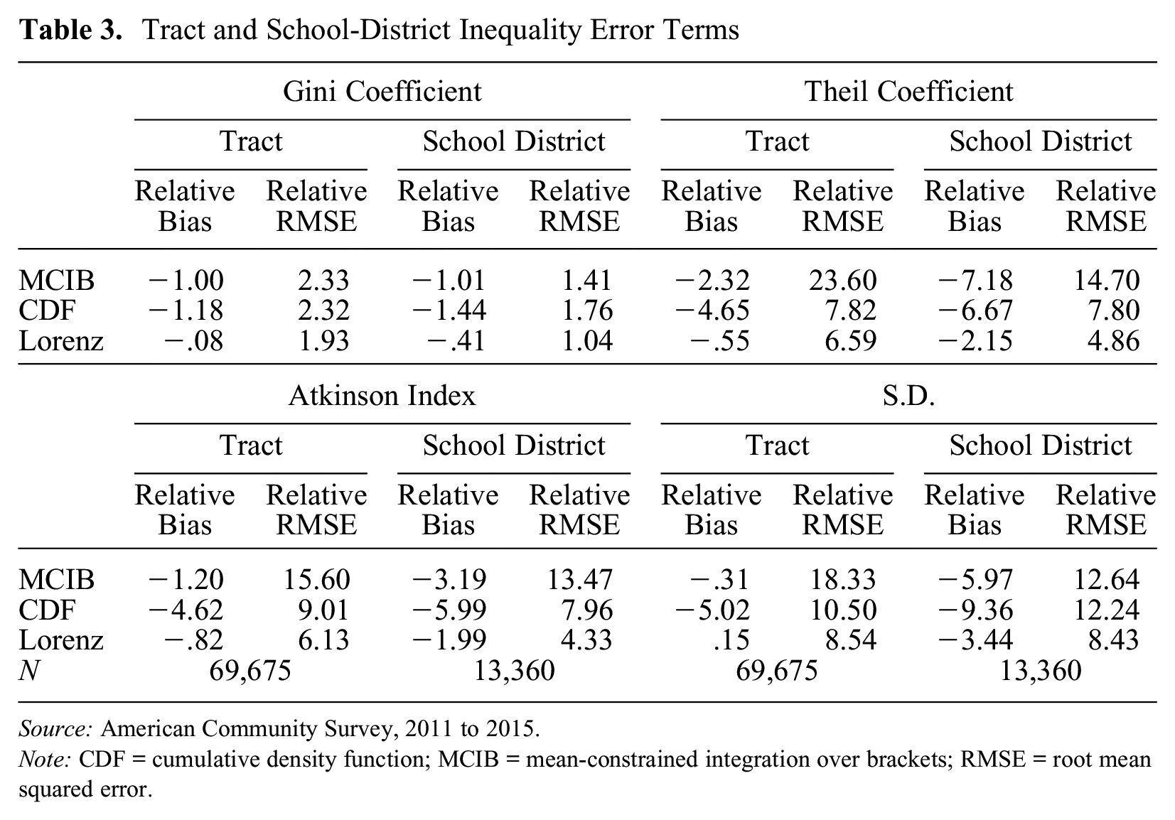
Table 3 shows the error terms for tract-level and school district–level estimates. Note the size of the relative RMSEs: these errors are larger for tracts than for school districts, and they are larger for school districts than for PUMAs. Comparing MCIB and CDF interpolation, the latter method produced Theil coefficient and Atkinson index estimates with lower relative RMSEs at the tract and school district levels. CDF interpolation also outperformed MCIB at estimating the standard deviation at the tract level, but the two methods performed comparably at the school district level. MCIB estimates tended to have lower relative bias than CDF estimates, but the relative RMSEs indicate this difference in bias is outweighed by the variance of the MCIB estimates.
Tract and School-District Inequality Error Terms
Source: American Community Survey, 2011 to 2015.
Note: CDF = cumulative density function; MCIB = mean-constrained integration over brackets; RMSE = root mean squared error.
Compared with MCIB and CDF interpolation, Lorenz interpolation produced slightly more accurate estimates of the Gini coefficient and significantly more accurate estimates of the Theil coefficient, Atkinson index, and standard deviation. At the school district level, Theil coefficient, Atkinson index, and standard deviation estimates based on Lorenz interpolation had 31 percent to 46 percent lower relative RMSEs than those based on the next best method, CDF interpolation. The gap between MCIB and Lorenz interpolation was even larger: the relative RMSEs from Theil coefficient, Atkinson index, and standard deviation estimates based on Lorenz interpolation were about 33 percent to 67 percent lower than those based on MCIB. Tract-level error metrics from Lorenz interpolation were also lower than those based on the other methods. However, these relative RMSEs were large (6.5 percent to 8.5 percent). Furthermore, these numbers do not account for sampling variation. For income data based on the five-year pooled ACS, the influence of sampling variation on tract-level estimates is substantial.
In summary, Lorenz interpolation, CDF interpolation, and MCIB produced accurate Gini coefficient estimates at the tract and school district levels. These methods seem to be up to the task of estimating income inequality measures that depend less on the upper tail of the income distribution. CDF produced more accurate estimates of the Theil coefficient, Atkinson index, and standard deviation than did MCIB, but Lorenz interpolation outperformed both methods at estimating these measures.
Quantile and Income Share Estimates from MCIB, CDF Interpolation, and Lorenz Interpolation
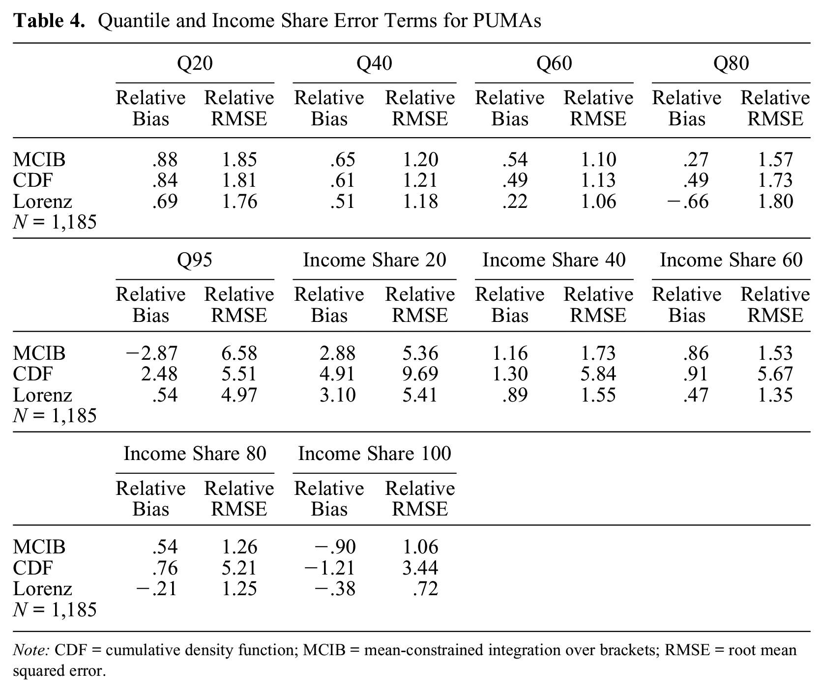
Table 4 shows relative bias and relative RMSE terms for MCIB, CDF interpolation, and Lorenz interpolation estimates of income quantiles and income shares. Income quantile estimates were produced for the 20th, 40th, 60th, 80th, and 95th percentiles of the income distribution at the PUMA level. Lorenz interpolation estimates had the lowest relative bias and RMSE for all percentiles except at the 80th percentile, where MCIB produced the most accurate estimates. Moving to income shares, I estimated statistics for each quintile of the income distribution. Lorenz interpolation produced the most accurate estimates of all quintiles except the bottom quintile, for which MCIB produced the most accurate estimates.
Quantile and Income Share Error Terms for PUMAs
Note: CDF = cumulative density function; MCIB = mean-constrained integration over brackets; RMSE = root mean squared error.
The greater accuracy of the Lorenz interpolation quantile estimates compared with CDF interpolation is particularly surprising given that the latter method derives income statistics from the CDF, which is the inverse of the percentile function. Note, however, that Lorenz interpolation estimates of the income quantiles and income shares were only slightly more accurate than CDF interpolation or MCIB estimates (a few hundredths of a percent in many cases). Although Lorenz interpolation can be used to estimate income quantiles, income shares, and other local statistics, its main utility is for estimating income inequality.
Discussion
I conclude with a discussion of the use cases of Lorenz interpolation, some contexts in which the method should not be applied, and some ways the method could be extended. Starting with use cases, Lorenz interpolation is a viable method for estimating income inequality at geographic levels that are not accounted for in census microdata but for which census summary table data are available. For instance, PUMS data only cover a subset of U.S. counties. 17 Researchers interested in examining income inequality for all U.S. counties must rely on grouped income data provided in census summary tables. For geographies such as these, including counties and census-designated places, using Lorenz interpolation on summary census data is a valid way to estimate income inequality.
Lorenz interpolation can also be used to estimate income distributions for geographies that are not provided in census data but can be approximated by aggregating incomes from a geographic level that is provided in the census. For example, Owens’s (2016) recent work on U.S. economic segregation, which is organized around school district boundaries, uses the robust Pareto-midpoint estimator (von Hippel et al. 2016), an improved version of the technique of imputing bracket midpoints for incomes in closed brackets and assigning a Pareto distribution mean to incomes in the top bracket. For a study such as this one, Lorenz interpolation would be a preferable method for estimating income inequality. Alternatively, researchers interested in the implications of income inequality for disparities in the quality of local public services may wish to approximate municipal income distributions by aggregating tract-level data to the municipal level. For such an analysis, Lorenz interpolation would yield more accurate estimates of municipal income inequality and should be used in lieu of Pareto-midpoint estimators and the other methods discussed here.
There are many use cases for Lorenz interpolation, but there are also situations where this method should not be used, either because the PUMS data are sufficient or grouped data are inadequate. For example, researchers who require income statistics at the metropolitan statistical area or state level should simply use PUMS data, which include geographic information for large regions such as metropolitan statistical areas and states. Conversely, although grouped income data are the only publicly available resource for studying incomes at lower geographic levels such as census tracts and blocks, researchers should be wary of estimating certain inequality measures from these data. The errors associated with tract-level Theil coefficient, standard deviation, and Atkinson index estimates produced in this analysis are too large for some analyses.
The large residuals of these estimates are even more concerning when one considers that census income data are sample data. Until 2000, these data were collected in the long-form portion of the decennial census, which is based on a sample covering approximately 18 percent of the U.S. population (Logan et al. 2018). Since then, income data have been collected in the ACS, which in its five-year form is based on a sample of about 5 percent of the population. Although the ACS provides error margins that can be used to construct 90 percent confidence intervals around the frequency estimates of each bin from the grouped income data, researchers have yet to develop methods for estimating income inequality that make use of these margins. The general approach has been to ignore them and work at a high enough geographic level that the error caused by sampling variation is negligible. 18
To improve on the method put forth in this article, researchers may want to consider using Bayesian methods to produce more reliable income inequality estimates for small areas. Empirical Bayes might be a viable method to supplement tract-level income data with information from neighboring regions. Note, however, that income data from the Census Bureau are already reweighted to incorporate demographic and other information from neighboring areas. Shrinking estimates from sparsely populated tracts toward the inequality levels of surrounding areas may have a limited effect on improving the reliability of estimates based on these data. Nonetheless, studies have successfully used Bayesian methods to improve small area estimates using census data from other countries’ national censuses (Assunção et al. 2005; Schmertmann and Gonzaga 2018). These methods may yield better estimators for small regions, particularly for unweighted income data.
Researchers should also evaluate the utility of Lorenz interpolation for estimating statistics from other kinds of grouped data. This study looked exclusively at income data from the census. Grouped data from this source are lower bound inclusive and upper bound exclusive. As a result, incomes that fall directly on an income boundary are assigned to the higher of the two bins subdivided by that boundary. This has a negative effect on the true bin means associated with the income groups. For data that apply different rules for handling incomes falling on the income boundaries, the improvement of Lorenz interpolation may be smaller. Researchers could determine this by comparing the performance of Lorenz interpolation, MCIB, and CDF interpolation using data from other national censuses.
Conclusion
In this article, I proposed a new method, Lorenz interpolation, for estimating income inequality from grouped income data. I showed that this method produces significantly more accurate and reliable estimates of income inequality at the PUMA, school district, and tract levels. I also showed that Lorenz interpolation produces slightly better estimates of income quantiles and income shares. Finally, I provided some scope conditions for the use of Lorenz interpolation. Although Lorenz interpolation produced more accurate inequality estimates at the tract level, these estimates are insufficiently reliable. Lorenz interpolation yielded more reliable estimates at the school district level. Lorenz interpolation especially outperforms the other methods at estimating income inequality measures such as the Theil coefficient that are sensitive to the upper tail of the income distribution. As the contribution of this upper tail to income inequality continues to grow (Piketty and Goldhammer 2014), methods for estimating these measures will become increasingly important.
Footnotes
Acknowledgements
I am grateful for the helpful comments of Martin Ruef, Colin Birkhead, William Grider, and members of the Duke Economic Sociology Workshop.