
Abstract
In the thriving field of network studies, there has been an emerging practice of comparing optimal modularity across social networks to evaluate the variation of network module–related substantive concepts, such as the level of consensus, polarization, or community boundary rigidity. This practice offers valuable insights and is often thoughtfully motivated, but it faces several conceptual and empirical challenges that merit careful consideration. Conceptually, the selected modularity metric may misalign with the substantive concepts researchers aim to measure. Empirically, estimated optimal modularity is highly sensitive to algorithm choice and to network characteristics unrelated to those substantive concepts, which can bias comparison results. The authors illustrate these issues with toy examples and systematic simulations and offer suggestions for more rigorous comparison practices. To show the practical significance of these lessons, the authors replicate an empirical study that examines the temporal trend of modularity scores for job mobility networks to evaluate the evolution of mobility boundary rigidity in the U.S. labor market.
Keywords
Network modularity, as formalized by Girvan and Newman (2002), is one of the most widely applied metrics for detecting and evaluating community structures in social networks. Drawing from its origins in complex systems and building on earlier social science traditions (e.g., Breiger, Boorman, and Arabie 1975; White, Boorman, and Breiger 1976), modularity has been increasingly adopted across diverse disciplines such as sociology, political science, and communication. Recent technical developments further enhance its applicability, including the introduction of LinkRank (LR) modularity for directed networks (Kim, Son, and Jeong 2010), generalized modularity for signed networks (He, Zhang, and Zhu 2023), stochastic blockmodeling (SBM) for inferential community detection (Peixoto 2023), and network-robust modularity measures (Botta and Del Genio 2016; Silva et al. 2022). These developments have facilitated an emerging practice: comparing optimal modularity scores across different social networks to assess temporal or cross-sectional variations in substantive concepts such as consensus (e.g., Jappe, Pithan, and Heinze 2018; Shwed and Bearman 2010), polarization/fragmentation (e.g., Dal Maso et al. 2014; Moody and Mucha 2013), and community boundary rigidity (e.g., Cheng and Park 2020; Lin and Hung 2022).
Many studies in this literature offer careful justification about the application of modularity in their research. Cheng and Park (2020), Shwed and Bearman (2010), and Jappe et al. (2018) provide thoughtful arguments about how variations of modular measures relate to their substantive concepts of interest. Despite these careful justifications, we find that comparing modularity across networks faces three interconnected challenges: (1) conceptual mismatch: modularity variation may not align with the substantive phenomena researchers aim to measure; (2) algorithm dependency: modularity estimates are highly sensitive to the choice of modularity metrics and community detection algorithms; and (3) network dependency: modularity scores vary systematically with network attributes (e.g., size, density, and community counts) that are often irrelevant to the substantive concepts.
If these issues are not sufficiently addressed, modularity comparison results may be implicitly biased. For instance, networks may appear to show increasing polarization when changes actually reflect methodological artifacts from varying network sizes; time-series analyses may detect spurious trends when the number of detected communities changes because of algorithmic sensitivity; and cross-sectional comparisons may yield misleading conclusions about levels of consensus or boundary rigidity when networks differ systematically in their densities. These problems are compounded when researchers use modularity-maximizing algorithms to both detect communities and measure their strength, creating circular dependencies that reduce comparability across networks.
To address these challenges, we recommend a multistep strategy toward more rigorous comparison following a systematic framework. First, assess conceptual alignment between the substantive concept and available modularity measures. If strong alignment exists with newer network-robust modularity measures, choose those measures; otherwise, use proper conventional measures such as Girvan-Newman (GN) or LR modularity. Second, address algorithm dependency by using non-modularity-based community detection algorithms to separate community detection from modularity estimation. Also, conduct robustness checks on algorithm and parameter selections. Third, address network dependency by standardizing the network size through bootstrapping rather than the widely applied reweighting method. Also, fix nodes across networks whenever proper. Fourth, validate findings with nonmodularity and domain-specific indicators, to ensure substantive conclusions are not driven by modularity-specific dependencies.
In summary, we provide systematic evidence of the pitfalls in modularity comparison and offer practical suggestions to mitigate these biases. The article proceeds as follows. We first review current applications of modularity comparison in social science research. We then discuss and reveal three major challenges in this comparative approach. Synthesizing these comparability issues, we next provide practical and concrete remedies. We illustrate the empirical significance of these lessons through a reanalysis of Cheng and Park’s (2020) influential study of U.S. labor market mobility.
Comparing Modularity Scores across Social Networks: Theoretical Motivations and Empirical Practices
Prevalence of This Comparative Practice in Social Science Research
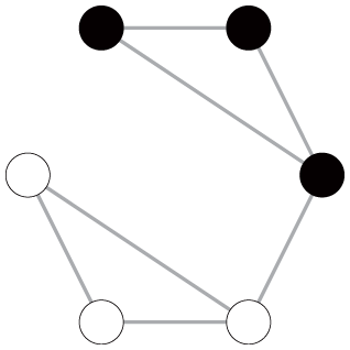
In network studies, the modularity score (Q), as a quality function, was developed and introduced by physicists (Girvan and Newman 2002; Newman and Girvan 2004) to find and evaluate community structures in networks. Since its inception, this quality function has quickly become the most widely applied technique to evaluate and detect a network’s modular structure (Fortunato and Barthelemy 2007). As illustrated in Figure 1, given a network, modularity scores vary across different partition/community division strategies. The higher the modularity score for a certain partition strategy, the better that partition captures the underlying modular structure. Therefore, by maximizing the quality function Q across all possible partition/community division strategies, scholars can detect the optimal partition/community structure of a network without any a priori assumptions about the number or size of communities.
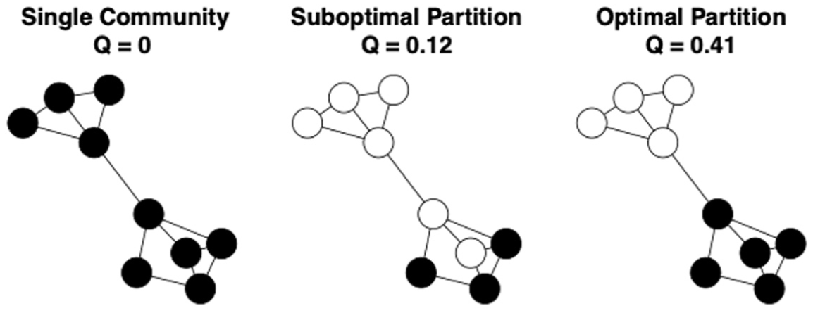
Rationale for using modularity scores to detect a network’s community structure.
Because the modularity score was designed to compare different partition strategies and search for the optimal one given a network, the most common early application in the social sciences was to detect the community structure of a given social network. For instance, Goldberg (2011) used modularity to detect the relational classes of a network constructed by individuals’ musical preferences, so as to reexamine the cultural omnivore thesis.
It is important to emphasize that the study of community structure has deep roots in social science research, predating recent developments in complex network analysis by several decades. Social scientists have long developed sophisticated techniques, including hierarchical clustering, blockmodeling, and structural equivalence analysis, for detecting and analyzing clusters, cliques, and structural positions in social networks (Freeman 1978; Wasserman and Faust 1994; White et al. 1976). These studies were explicitly acknowledged in Girvan and Newman’s (2002) original paper. However, the practice we examine here is not community detection itself but the specific application of comparing modularity scores across different social networks to make substantive claims about temporal or cross-sectional variations in social processes.
Use of this comparative application has grown over the past two decades (e.g., Cheng and Park 2020; Lin and Hung 2022; Majó-Vázquez, Nielsen, and González-Bailón 2019; Moody and Mucha 2013; Shwed and Bearman 2010). Shwed and Bearman (2010) carefully justified this extended application. The basic idea is, because the modularity score indicates the salience of a network’s modular structure, we can evaluate the variation in the modular salience across networks by comparing the modularity scores of different networks’ optimal partitions, which reflects the variation in the module-related features of interest. Figure 2 illustrates the rationale (adapted from Shwed and Bearman 2010, Figure 2). The optimal partition/community structure is the same for the three networks, but the corresponding modular scores decline with the increasing connectedness among communities.
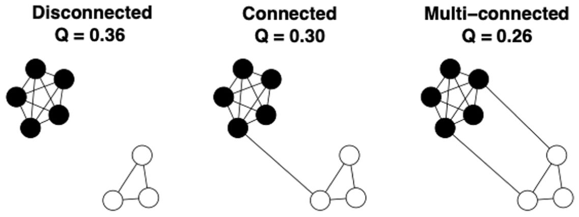
Rationale for comparing modularity scores across social networks.
This extended application is inspiring. Soon after its introduction, comparing modularity scores across networks became prevalent across social science disciplines. For instance, some researchers compared the modularity scores of scientific citation networks over time to evaluate the evolution of scientific consensus (e.g., Bruggeman, Traag, and Uitermark 2012; Jappe et al. 2018; Shwed 2015; Shwed and Bearman 2010). Political scientists and communication scholars compared the modularity scores of political networks over time and across regions to evaluate the evolution and variation of political polarization and fragmentation in various cultural settings (e.g., Dal Maso et al. 2014; Moody and Mucha 2013; Porter et al. 2007). Sociologists compared the modularity scores of job mobility networks over time to evaluate the evolution of the rigidity of occupational class boundaries (e.g., Cheng and Park 2020; Lin and Hung 2022). Table 1 summarizes the most representative studies.
Summary of Social Science Articles That Compare Modularity Scores across Social Networks.
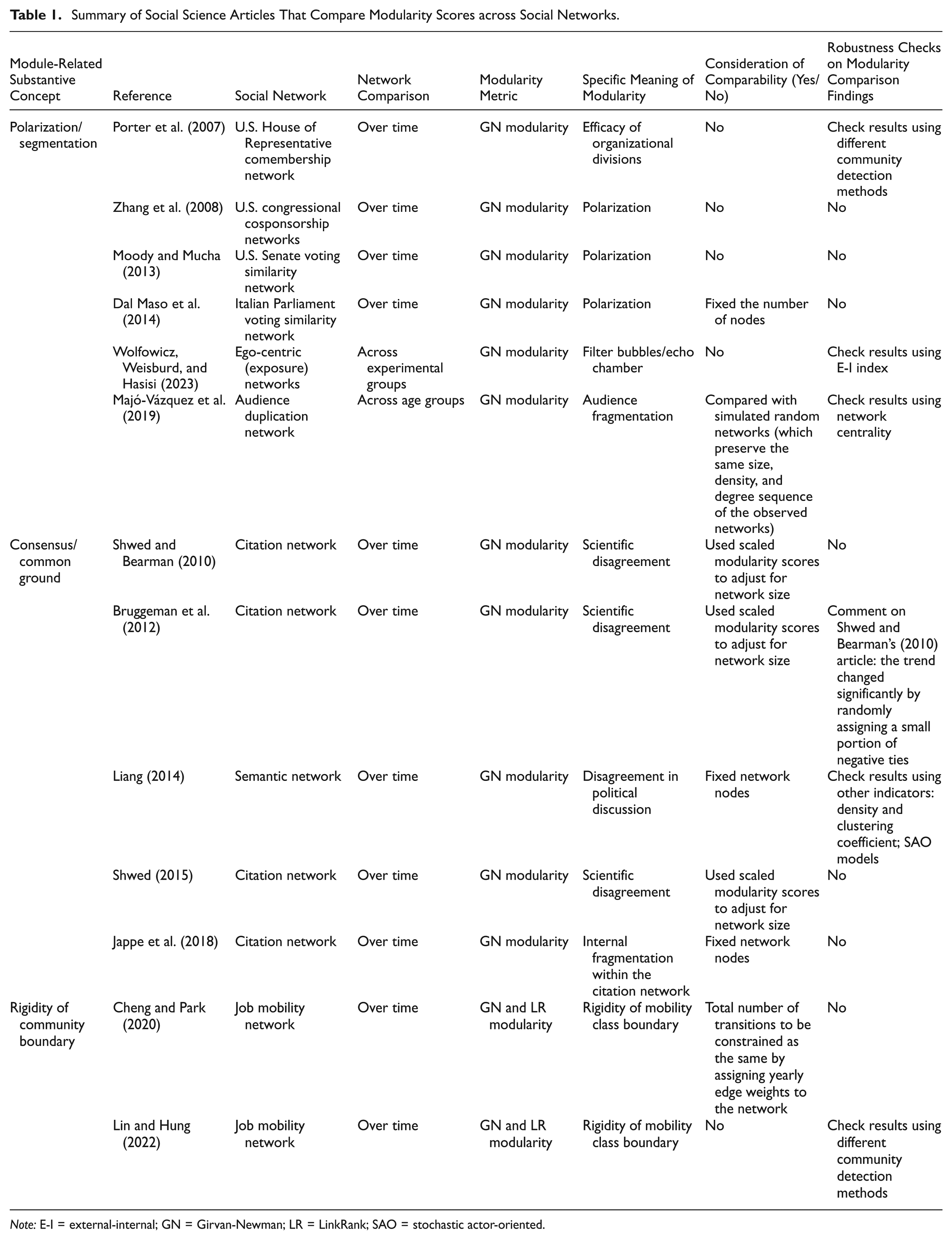
Note: E-I = external-internal; GN = Girvan-Newman; LR = LinkRank; SAO = stochastic actor-oriented.
Theoretical Motivations and Empirical Strategies
As shown in Table 1, theoretically, scholars are interested in three major substantive concepts when comparing modularity scores across social networks. The first is the variation of polarization or fragmentation levels, where higher modularity indicates greater polarization or fragmentation (e.g., Majó-Vázquez et al. 2019; Wolfowicz et al. 2023; Zhang et al. 2008). The second is the variation of consensus or common ground, where declining modularity signals consensus formation (e.g., Jappe et al. 2018; Liang 2014; Shwed 2015; Shwed and Bearman 2010). The third is the variation of community boundary rigidity, where rising modularity suggests increasing boundary impermeability (e.g., Cheng and Park 2020; Lin and Hung 2022).
Empirically, there are two major modularity metrics in the existing literature. The dominant one is the Girvan-Newman function and its derivatives (Girvan and Newman 2002; Newman and Girvan 2004). These measures capture the difference between the density of edges in communities given a partitioning strategy and that expected if the edges were connected at random. The larger the difference, the greater the deviance of that community division from a random graph. As Newman and Girvan (2004) note, “the height of a peak is a measure of the strength of the community division” (p. 7). For weighted and directed graphs, the formula is
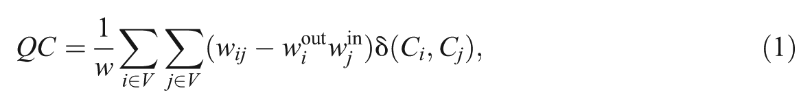
where V is the node vector and W is the weighted adjacency matrix of the focus network. i and j are the indices of the nodes, and wij stands for the (i, j)th entry in W.
Because GN modularity may not sufficiently account for the edge directions, LR modularity was developed to detect the modular structure of directed networks (Kim et al. 2010). This modularity measure incorporates the idea of Google’s PageRank algorithm (Brin and Page 1998). For weighted and directed graphs, it can be formulated as
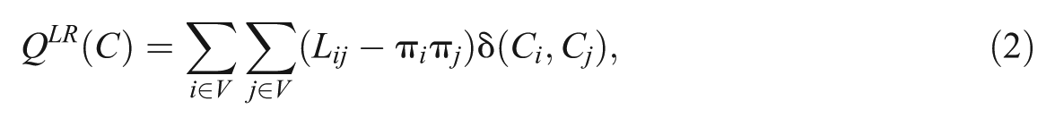
where Lij = πigij. gij is the (i, j)th entry of the adjacency matrix G with row normalization, and π i is the ith element of the PageRank vector that satisfies πT = πTG. Compared with GN modularity, scholars argue that LR modularity is not only more suitable for directed graphs but also better for capturing the multistep moves (i.e., indirect pathways or sequential transitions that span multiple steps rather than direct connections between nodes) on the networks (Cheng and Park 2020; Kim et al. 2010). Essentially, GN modularity is equivalent to the well-known notion of assortativity (here the categorical variables are the communities), and LR modularity is equivalent to the earlier defined Markov stability (for more detailed discussions, see Lambiotte, Delvenne, and Barahona 2009).
Existing Considerations of Comparability Issues
The reviewed studies demonstrate thoughtful motivations and justifications for why modularity comparison is relevant to their research. Moreover, some studies were already aware of the comparability issues and implemented partial fixes, such as adjusting for network size or fixing nodes, to improve estimation reliability (e.g., Jappe et al. 2018; Liang 2014; Shwed 2015; Shwed and Bearman 2010).
Despite these efforts, these strategies cannot fully address the comparability issues. There remain opportunities for additional systematic considerations of how modularity varies across empirical networks and how its alignment with substantive concepts changes accordingly.
Are Modularity Scores Comparable across Social Networks? Conceptual and Empirical Issues
When modularity was developed and introduced in network studies, its major function was to help detect the optimal modular structure within a network. Hence, if we compare modularity scores across different networks, various conceptual and empirical issues can arise and bias our findings. In this section, we discuss these issues using toy examples for easier illustration, and we elaborate on the empirical issues using systematic simulations in the subsequent section.
Conceptual Issues
Conceptually, an important consideration is that the terms commonly measured by modularity scores, such as “consensus,”“partition/polarization,” and “community boundary rigidity,” although all related to networks’ modular structures, are theoretically distinct concepts. They emphasize different aspects of a network’s modular structure.
Specifically, “community boundary rigidity” refers to the impermeability of community borders to flows or exchanges. This concept emphasizes the low rates of cross-community ties or intergroup mobility: the low degree of transitivity among communities. “Polarization” or “partition/segmentation” is the presence of internally cohesive groups that are distant from or opposed to one another. “Partition/segmentation” and “polarization” are also different from each other; for instance, in scientific citation networks, specialization across research areas (“partition/segmentation”) may not suggest antagonistic camps (“polarization”). Here, we group them together because they both emphasize not only the transitivity (in whatever form; antagonistic ties would suggest even less transitivity) among communities but also the level of cohesiveness within each community. 1 “Consensus,” in contrast, refers to the degree to which the network shares a common ground, or the concentration of actors or ties around a dominant community. Thus, it concerns not only transitivity among and cohesiveness within communities but also the concentration pattern across communities: whether the network coalesces around dominant groups or remains diffuse. In summary, all these concepts are relevant to the salience of networks’ modular structures, but they are inherently different. With careful research design, appropriate metric selection, and domain-specific interpretation, modularity can inform all these concepts. However, it would be problematic to evaluate these substantively distinct concepts by merely emphasizing the modular salience across networks.
To illustrate the significance of this conceptual problem, Table 2 provides two networks (graphs A and B) under three different hypothetical scenarios in which modularity is used to capture different substantive concepts. Both networks have six nodes and three disconnected communities. The only difference is that in graph A, all communities have two edges, and in graph B, a dominant community has 20 edges. Given these two hypothetical networks, we can consider the following three scenarios.
Scenario 1: Modularity scores are used to capture the boundary rigidity of mobility classes/communities. The networks are viewed as job mobility networks, the nodes represent six different occupations, and the edges indicate the number of mobility events (in hundreds) among occupations. Graphs A and B depict the mobility situations in years T and T + 1, respectively. In year T, there are 600 mobility events, confined to three communities. In year T + 1, although the community structure does not change, job mobility becomes much more frequent in one community. The number of mobility events between occupations represented by black nodes increases from 200 to 2,000. Suppose the total number of people in the labor force stays constant, under this scenario, although the fluidity of the overall labor market increases, the community boundary rigidity remains the same because there is no cross-community event in both graphs. Accordingly, if modularity scores capture the rigidity of the community boundary, they should be the same across these two networks.
Scenario 2: Modularity scores are used to capture the level of audience fragmentation, as indicated by the sharing of media outlets among audiences. The networks refer to audience duplication networks, the nodes represent six different media outlets, and the edges measure the size of the shared audience (in thousands) (i.e., audience duplication) among these media outlets. Again, graphs A and B provide the audience duplication situations in years T and T + 1. In year T, we have six media outlets form three communities, and there are 2,000 shared audiences within each community. In year T + 1, the six media outlets also form three communities; however, in one community, the two outlets have highly overlapping audiences (20,000) and thus form a distinct group vis-à-vis the other two groups. Assume that the total size of the audiences stays the same over time, under this scenario, audience fragmentation becomes more salient because the strong tie between the media outlets represented by the black nodes in graph B indicates the audiences have a strong tendency toward self-selection (Majó-Vázquez et al. 2019) and become less likely to be integrated/merged into other communities than in graph A. Hence, if modularity scores accurately capture such dynamics, they should increase from graph A to graph B.
Scenario 3: Modularity scores are used to measure the level of scientific consensus/agreement. The networks represent the citation networks regarding contestable scientific topics, the nodes represent six well-known research teams on that topic, and the edges indicate the number of positive citations among them (Bruggeman et al. 2012; Shwed and Bearman 2010). Also, graphs A and B show the citation networks in the years T and T + 1. In year T, there are six published papers, and their citation networks form three communities (like three dominant schools on that topic). In year T + 1, a breakthrough is made by the teams represented by the black nodes, and they have 18 new back-to-back publications citing each other’s work. In this scenario, the scientific consensus about that contestable topic should have increased because the breakthrough is substantial. Accordingly, if modularity captures network consensus, the modularity score should decline from graph A to graph B because of the decreasing disagreement.
Toy Examples Showing the Conceptual Issues with Three Hypothetical Scenarios.
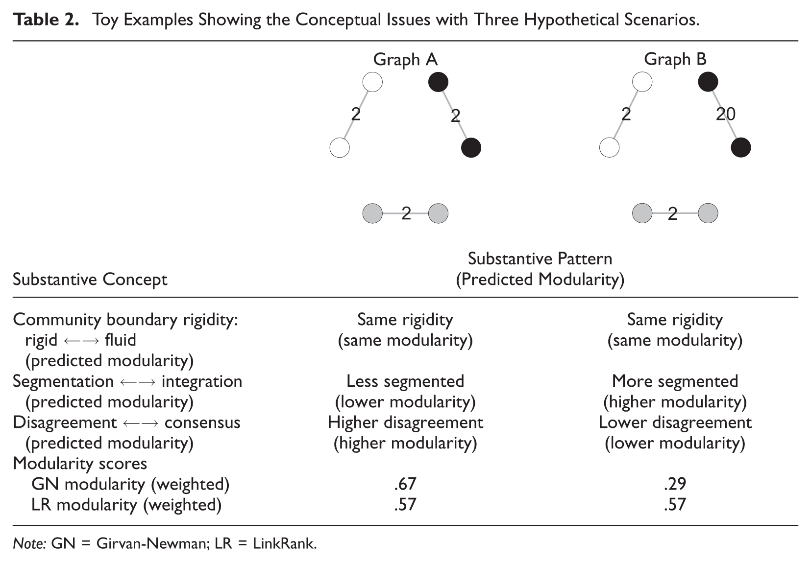
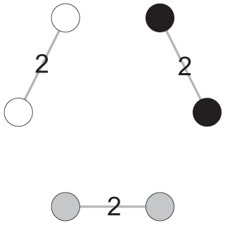
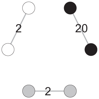
Note: GN = Girvan-Newman; LR = LinkRank.
In summary, these hypothetical scenarios reveal that, conceptually, the same variation of network patterns can be explained very differently when referring to different substantive concepts, which leads to different predictions of modularity change. The lower panel of Table 2 provides the GN and LR modularity scores for both graphs. As clearly shown, while GN modularity increases, LR modularity stays the same from graph A to graph B. In other words, using different modularity metrics will produce completely different empirical evidence. This finding leads us to further examine the empirical issues concerning modularity comparison across networks.
Empirical Issues
Empirically, an important consideration is that the commonly used modularity metrics (both GN and LR functions) are highly sensitive to various network characteristics that are irrelevant to the substantive concepts in which social scientists are interested, such as network size (i.e., total number of nodes and edges) (Fortunato and Barthelemy 2007) and number of communities. Moreover, as indicated in Table 2, different modularity metrics may also react to the same variation of network patterns in different ways. Altogether, these problems can bias our comparative findings and make the corresponding interpretations difficult.
To illustrate these empirical issues, we extend the six-node toy examples by imposing some carefully designed variations in network characteristics, as shown in Table 3. Specifically, we provide four pairs of networks (i.e., graphs 1 and 2, 3 and 4, 5 and 6, and 7 and 8) with two basic settings: one with two communities (upper panel) and the other with three communities (lower panel). The networks in each pair have the same number of nodes, total edge weights, node degree distribution, and level of community connectedness. The community memberships of nodes are predefined before calculating modularity.
Toy Examples Showing the Empirical Issues of Modularity Comparison
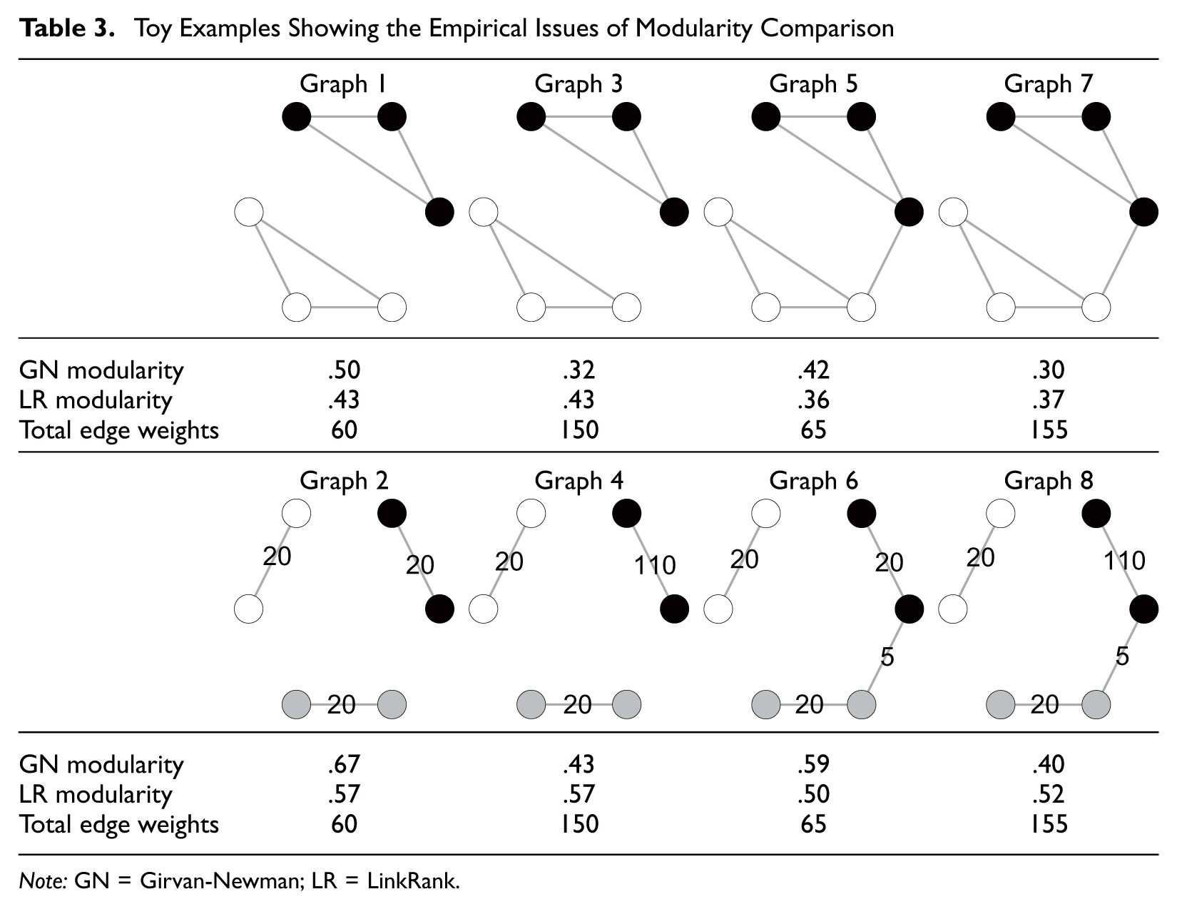
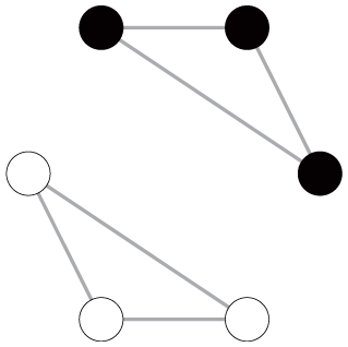
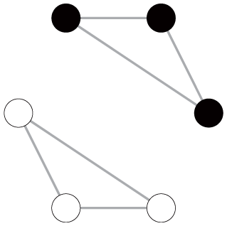
Note: GN = Girvan-Newman; LR = LinkRank.
These toy examples yield two key observations. First, ceteris paribus, both GN and LR modularity increase with the number of communities, even though the level of community connectedness is the same across networks. We can see this by comparing the GN and LR modularity scores within each network pair (i.e., graph 1 vs. graph 2, graph 3 vs. graph 4, graph 5 vs. graph 6, and graph 7 vs. graph 8). Second, GN and LR modularity react to the emergence of dominant communities in systematically different ways. Particularly, ceteris paribus, for networks with only disjointed communities, the emergence of dominant communities tends to decrease GN modularity but has no influence on LR modularity. This observation can be drawn by comparing the modularity scores of the graphs in the second column to graphs in the first column (graph 3 vs. graph 1, graph 4 vs. graph 2). However, for networks with connected communities, the emergence of a connected dominant community decreases GN modularity but slightly increases LR modularity, as reflected by the modularity scores of the graphs in the fourth column in contrast to those in the third column (graph 7 vs. graph 5, graph 8 vs. graph 6). If the emergence of the dominant communities is coupled with the change in the level of community connectedness, the divergent responses of the GN and LR modularity metrics to the variation of network patterns become more salient (see the modularity comparison of graphs 3 vs. graph 5 and graph 4 vs. graph 6).
Overall, this series of toy examples demonstrates the network and algorithm dependency issues of modularity comparison. On the one hand, the optimal modularity can change systematically across networks with various features that may be irrelevant to our focus substantive concepts. On the other hand, different modularity metrics can react to the same structural changes in networks in systematically different ways. If these issues are not sufficiently addressed, modularity comparison across networks can lead to misleading conclusions about network dynamics.
Network and Algorithm Dependency of Modularity Comparison: Systematic Simulations
Cautions in Previous Network Studies
We are not the first to notice the above-mentioned empirical issues. Even before modularity’s formalization, researchers working with community detection methods—blockmodeling, structural equivalence, and clique detection—recognized that comparing network structures across graphs required careful attention to network size, density, and sampling properties (Breiger et al. 1975; Freeman 1978; Wasserman and Faust 1994; White et al. 1976). Contemporary discussions of modularity’s limitations in complex networks further elaborated these concerns (Fortunato and Newman 2022), focusing particularly on the technical properties of GN modularity and problems related to community detection and modular measurement.
First, GN modularity is not standardized, as random graphs can have nonzero modularity scores (Guimerà, Sales-Pardo, and Nunes Amaral 2004; Peixoto 2023). Therefore, even across networks with the same degree of modular structures, modularity scores may differ because of random variations in sparse graphs. Second, GN modularity has an intrinsic scale proportional to
Although LR modularity accounts for edge direction, many issues in GN modularity may also apply to LR modularity. Moreover, as shown in Table 3, GN and LR modularity change in different directions when measuring the same network dynamics, suggesting they may capture different aspects of a network’s modular structure. This indicates that different modularity metrics can provide systematically different comparison results, adding additional complexities to modularity comparison across social networks.
Illustrations Using Systematic Simulations
Given this long-standing awareness of the intricacies of comparing modularity across networks, many empirical studies use multiple community detection algorithms to evaluate the robustness of their findings (e.g., Lin and Hung 2022; Porter et al. 2007). Nonetheless, we still lack systematic evidence of the network and algorithm dependency issues in modularity comparison. The six-node toy examples provide suggestive evidence, but they only allow examination of (1) a few well-designed network structures, (2) limited variation of the number of nodes and edges, and (3) limited variation of community structures. Hence, to illustrate how GN and LR modularity change systematically with what network characteristics, we offer more comprehensive simulations controlling for the salience of the modularity structure with two setups: (1) random graphs, which theoretically have no modular structure and (2) graphs with only disjointed communities, which theoretically have the most clear-cut modular structure.
Figure 3 summarizes the findings of the systematic simulations on random graphs generated on the basis of the Erdős-Rényi and Barabási-Albert templates. 2 The simulations show how GN (left column) and LR (right column) modularity scores change with certain network characteristics and algorithms. We focus on the effects of (1) number of nodes, (2) number of edges, (3) random graph–generating algorithms, and (4) community detection algorithms. The technical details are provided in the note to Figure 3, Appendix A in the online supplement, and our replication package.
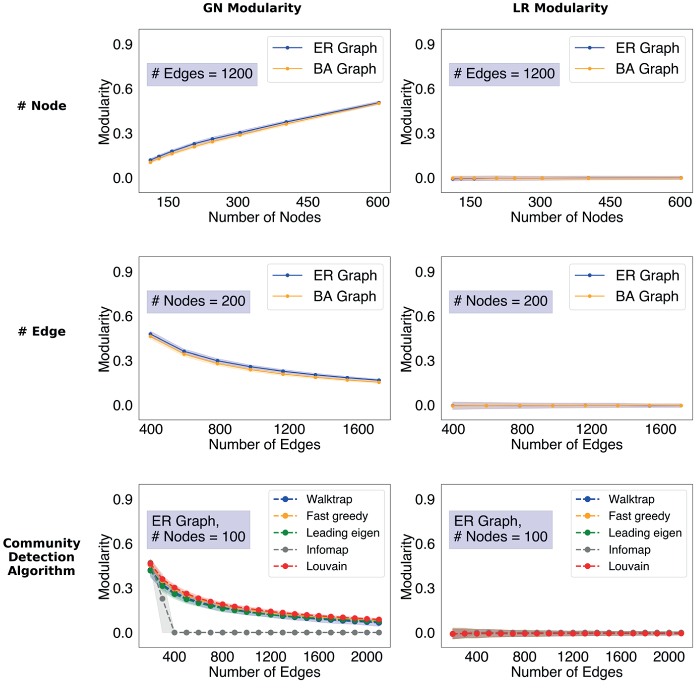
Illustrations from systematic simulations: random graphs.
This series of simulations yields two key findings. First, GN and LR modularity react to network characteristics and algorithmic choices in systematically different ways. Specifically, ceteris paribus, for both Erdős-Rényi and Barabási-Albert random graphs, GN modularity (1) increases with node counts (first row), (2) decreases with edge counts (second row), and (3) changes with community detection algorithms (the third row), but these factors do not influence LR modularity. In this sense, compared with GN modularity, LR modularity is more standardized and much less likely to produce false positives for random graphs, which should contain no modular structure.
Second, ceteris paribus, among the five commonly used community detection algorithms, Infomap has the fastest speed of converging GN modularity scores to zero with the increase in edge counts (the third row). In other words, Infomap—the only algorithm that does not aim to detect communities by maximizing modularity—is most effective at identifying random graphs, making it less likely than the other four algorithms to produce false positives.
Figure 4 summarizes the findings of the systematic simulations on the graphs with disjointed communities. In this set of simulations, we examine how GN (left column) and LR (right column) modularity change with the following network characteristics: (1) number of nodes, (2) number of edges, (3) number of communities, (4) edge distribution across communities, and (5) node distribution across communities. The technical details are provided in the note to Figure 4, Appendix A in the online supplement, and our replication package.
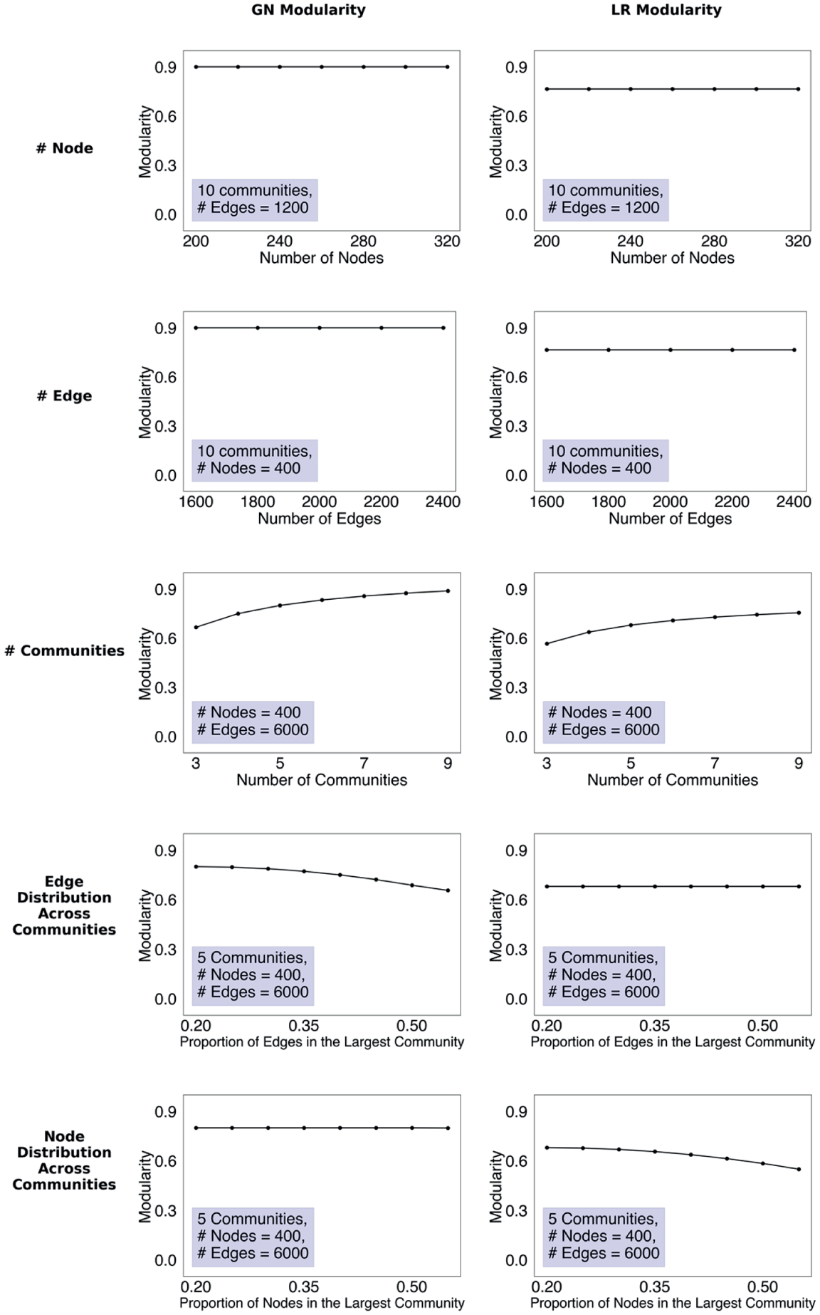
Illustrations from systematic simulations: graphs with disjointed communities.
These simulations yield three main findings. First, neither GN nor LR modularity is influenced by network size. Particularly, ceteris paribus, the increase in node counts (the first row) or edge counts (the second row) has no influence on GN or LR modularity. Second, ceteris paribus, both GN and LR modularity increase monotonically with the number of communities (the third row). Third, GN and LR modularity react to the edge and node distribution across communities in systematically different ways. Specifically, ceteris paribus, the more unequal the distribution of edges across communities (measured by the ratio of the largest community’s edges over the total number of edges), the lower the GN modularity scores are; there is no change in LR modularity (the fourth row). In contrast, the increase in the unevenness of node distribution across communities (measured by the ratio of the largest community’s nodes over the total number of nodes) has no influence on GN modularity but tends to decrease LR modularity (the fifth row). These results suggest GN and LR modularity respond differently to the node and edge distribution across communities, which indicates they would be suitable for capturing different modular-related substantive concepts.
To assess the robustness of our findings, we replicate Figures 3 and 4 using alternative parameter settings, varying node, edge, community counts, and number of simulated graphs. The results are presented in Figures A1 and A2 in the online supplement. To address concerns regarding the resolution limit of the Louvain algorithm, we also conduct analyses that alter the resolution and seed parameters when detecting communities in random graphs. Figure A3 in the online supplement reports results under alternative specifications: (1) resolution = 0.5 and (2) resolution = 2.0, which are the commonly discussed extremes of the resolution parameter (Fortunato and Barthelemy 2007). The results are largely consistent with the qualitative patterns of our main conclusions.
Careful readers may question why GN and LR modularity would display significant differences in our systematic simulations, considering all simulated networks are undirected. In particular, when Kim et al. (2010) formalized LR modularity, they showed it could be reduced to GN modularity for undirected networks. We note that this equivalence was derived on the basis of an implicit assumption that the network should be a nonrandom graph with well-connected communities. To show this, we extend the analyses in Figure 4 by adding cross-community edges randomly in our simulated graphs, and we present the results in Figures A4 (ratio of cross-community edges = 0.05) and A5 (ratio of cross-community edges = 0.2) in the online supplement. The results illustrate that when the cross-community ratio is low (Figure A4) and the simulated graphs have clear-cut community structures like the disjointed graphs, the differences between LR and GN modularity maintain. However, as the simulated graphs become fully connected (Figure A5), the patterns of LR modularity converge to those of the GN modularity; they are both affected by edge distribution but stay constant across node distribution.
To summarize, these systematic simulations illustrate the network and algorithm dependency of modularity comparison. The estimated optimal modularity can vary systematically with (1) network characteristics, including the number of nodes, edges, and communities, and node and edge distribution across communities, and (2) algorithmic choices, including random graph–generating algorithms, community detection algorithms, and modularity metrics, even if the salience of the modular structure is the same in the network’s generating process. These issues merit more attention toward reliable modularity comparison results when measuring substantive structural dynamics.
Alleviate Comparability Issues: A Multistep Framework
The previous two sections reveal three major issues of comparing modularity across social networks: concept mismatch, algorithm dependency, and network dependency. Here, we propose a multistep framework to address these issues in a sequential manner, ensuring more rigorous and reliable comparison. We summarize these issues and our respective recommendations in Table 4 and present the multistep decision framework in Figure 5.
Recommendations on Robustness Checks and Alternative Metrics.
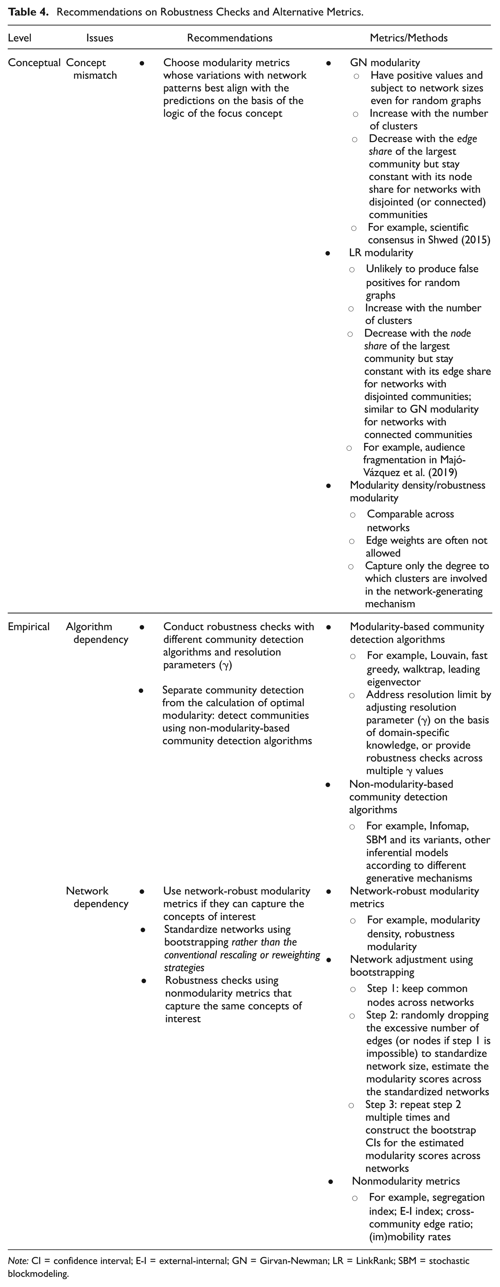
Note: CI = confidence interval; E-I = external-internal; GN = Girvan-Newman; LR = LinkRank; SBM = stochastic blockmodeling.
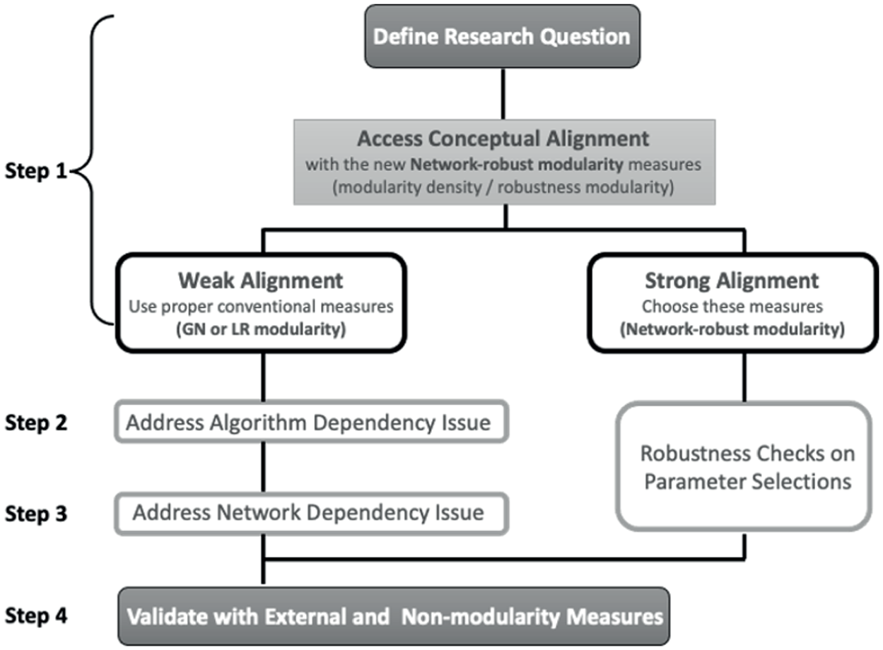
A multistep framework for rigorous modularity comparisons across social networks.
Assess Conceptual Alignment
First and foremost, regarding concept mismatch, we recommend carefully choosing among different modularity metrics and using the one whose variations with network patterns best align with the predictions based on the logic of the focus concept. Even though it is nearly impossible to provide a comprehensive map that bridges modularity metrics and substantive concepts, we may start from some common scenarios based on our toy examples and simulations. In Table 4, we summarize the systematic differences for the two dominant modularity metrics (i.e., GN and LR modularity) and the newer network-robust modularity metrics (i.e., robustness modularity and modularity density) in their reactions to variations in network patterns. For example, although the edge share of the largest community decreases GN modularity regardless of the connectivity across communities, its impact on LR modularity depends on the connectivity across communities. These different patterns hint that GN modularity could be more appropriate to capture the degree of scientific consensus, and LR modularity might be better for measuring audience fragmentation or the rigidity of community boundaries. Researchers may also consider network-robust modularity measures, which are specifically designed for cross-network comparison (e.g., Silva et al. 2022). We will discuss their pros and cons later.
Address Algorithm Dependency
Regarding algorithm dependency, the existing strategy is to conduct robustness checks using different community detection algorithms (e.g., Lin and Hung 2022). We agree with this strategy, but we further recommend to separate community detection from modularity estimation by using non-modularity-based community detection algorithms.
Many studies combine these two processes: they first maximize modularity to detect a network’s optimal community structure, and then use the resultant modularity to evaluate the salience of that network’s module-related attributes. This practice may aggravate the comparability issues, because both (1) the modularity metric’s capacity to correctly detect community structure and (2) its accuracy to measure the substantive concept vary systematically across networks. Additionally, as mentioned earlier, these modularity-based community detection algorithms are subject to the “resolution limit” problem. To address this issue, resolution-adjusted modularity (Newman 2016) provides one theoretically principled approach, serving as the maximum likelihood estimator for community structures. However, this approach requires careful selection of resolution parameter (γ), which remains an open methodological question requiring domain-specific justification or robustness checks across multiple γ values. 3
The modern community detection view, like SBM and the Infomap algorithm, aims to estimate the preferential linking patterns through stochastic transition matrices (Peixoto 2023). Specifically, these inferential approaches define community structure through a generative model, which outlines how a latent partition of nodes influences the links. The key inference here is to identify the most possible node partitions given the observed network. When the model fits the data well, the generative mechanism explains the observed communities. 4 These non-modularity-based inferential algorithms allow researchers to separate community detection from modularity estimation. They are less likely to generate false positives for random graphs (as indicated by the performance of the Infomap algorithm in Figure 3) and can better identify small or overlapping communities than can the modularity-based ones. Once the communities are correctly detected, modularity metrics specific to different social phenomena can be further applied.
Address Network Dependency
Regarding network dependency, scholars could consider using the recently developed network-robust modularity metrics (e.g., Silva et al. 2022). One example is modularity density (Botta and Del Genio 2016). By incorporating community density and cross-community edges into the modularity functions, modularity density allows a direct quantitative comparison of the community structure across networks of different sizes. Another example is robustness modularity (Silva et al. 2022), which is based on the difference between the real network and corresponding random networks.
However, these measures are not a panacea. Although comparable across networks, they have significant limitations (see Table 4). First, many of them are not designed for weighted networks and cannot account for the edge weight distribution. For example, robustness modularity needs to randomly permutate the edges, but it is unclear how to permutate the edge weights. Isolates are not even allowed in modularity density calculation. Therefore, if we want to apply these newly developed network-insensitive modularity metrics, we need to first convert weighted graphs to unweighted ones. This conversion will introduce another intricacy in choosing the threshold for dichotomization. Several studies have examined the consequences of various filtering/dichotomization strategies. Mukerjee et al. (2022) focus on filtering strategies for bipartite projections in co-exposure networks, and Gomes Ferreira et al. (2022) and Neal (2022) provide more comprehensive reviews of network filtering and thresholding techniques across a wider range of network types and contexts. Second, the network-insensitive modularity measures do not solve conceptual mismatch issues; they may not capture the theoretical concepts that scholars are interested in. To some extent, robustness modularity is good for evaluating the degree to which a cluster is involved in the generating mechanism of a network, rather than the level of consensus or the rigidity of the cluster’s boundary in the network. Even normalization based on null models does not solve this issue, because it only tells the existence of a modular structure, instead of which network partition is more likely (Peixoto 2023).
Therefore, if we must use network-sensitive modularity metrics (e.g., GN and LR modularity) to better capture the concepts of interest, we should use appropriate network standardization to increase modularity comparability across networks. In this regard, our foremost warning is that the conventional rescaling and reweighting strategies (e.g., Cheng and Park 2020; Shwed 2015; Shwed and Bearman 2010) cannot sufficiently address the network dependency issue, because there is a high level of interdependency among various network characteristics (e.g., the number of nodes and edges can affect the number of communities identified). We would suggest the following strategies.
First, fix nodes whenever possible, as that will solve most problems. For some studies, the nodes are the same across networks (e.g., academic journals in citation networks and Congress members in political networks), making modularity comparison more reliable.
Second, standardize the number of nodes and edges (weights) using bootstrapping. The simple strategy of rescaling or reweighting the network size is not a good remedy because it assumes the number of nodes and edges does not influence other network characteristics. It would be more accurate to capture the robust network structure by randomly dropping excessive nodes or edges and to get bootstrapping distributions of the estimated modularity scores.
Validate with External and Nonmodularity Measures
Finally, robustness checks should be conducted using non-modularity-related metrics that also capture the substantive concepts of interest. For instance, some simpler metrics like the immobility rate (i.e., the stayer ratio in the case of mobility networks) may effectively capture the rigidity of mobility boundaries. Similarly, we could use existing metrics, like the segregation index and the external-internal (E-I) index, to measure fragmentation. The E-I index, defined as (external ties − internal ties)/(external ties + internal ties), was developed by social scientists decades before network modularity (Krackhardt and Stern 1988) and measures the relative volume of external ties (between groups) to internal ties (within groups). The segregation index (Freeman 1978) also measures the extent to which ties occur within versus between groups, but compares observed patterns to what would be expected under random mixing. The limitations of these measures are that they all require predefined group membership, whereas modularity can detect communities algorithmically. Moreover, when comparing across networks, they may also be sensitive to network size, density, relative group sizes, and so on (Hanneman and Riddle 2005; Tóth et al. 2021). However, these indices offer certain advantages; simpler calculations reduce algorithm dependency and improve interpretability, and predefined group membership avoids resolution limit problems. For studies examining concepts like mobility rigidity or political fragmentation, where group boundaries are theoretically meaningful, these indices could serve as valuable robustness checks alongside modularity measures.
A Multistep Decision Framework
To help researchers navigate these recommendations, we synthesize them into a systematic multistep framework, illustrated in Figure 5.
Step 1: Define the research question and assess conceptual alignment. As summarized in Table 4, assess whether your concept aligns with network-robust measures (modularity density or robustness modularity) or conventional measures (GN or LR modularity). If you have strong alignment with network-robust measures, choose them while addressing their limitations with weighted networks. Otherwise, use GN modularity for consensus-related concepts or LR modularity for fragmentation/rigidity concepts.
Step 2: Address algorithm dependency. Separate community detection from modularity measurement by using non-modularity-based community detection algorithms when proper. Conduct robustness checks across different algorithms and parameter settings.
Step 3: Address network dependency and apply size and density corrections. For conventional measures, fix common nodes whenever possible, use bootstrap simulations to equalize edge and node counts, and avoid simple rescaling. For network-robust measures, conduct robustness checks on parameter selection as needed.
Step 4: Validate with external and nonmodularity measures. Use simpler nonmodularity and domain-specific indicators to ensure the findings reflect genuine social processes rather than methodological artifacts.
In summary, despite the intricacy of modularity comparison, we acknowledge the value of this application in social network research. With this list of suggestions, we aim to improve the rigor of this application and the solidity of the related findings.
Practical Relevance: Reexamine the Mobility Boundary Rigidity in the U.S. Labor Market, 1989 to 2015
The Empirical Case
To illustrate the practical significance of our suggestions, we replicate a study published in the American Journal of Sociology (Cheng and Park 2020) that uses LR modularity to evaluate the mobility boundary rigidity in the U.S. labor market between 1989 and 2015. This study is a careful and influential application of modularity comparison. We reexamine it to show how additional attention to comparability issues can affect substantive findings even when researchers take reasonable precautions.
Cheng and Park (2020) did not rely on predefined occupational classes and conventional analytic techniques (e.g., log-linear models) in the occupational mobility literature (e.g., Jarvis and Song 2017). Instead, drawing on the 1989–2015 March Annual Social and Economic Supplement of the Current Population Survey (Flood et al. 2017), Cheng and Park innovatively constructed occupational mobility networks for each survey year. In each network, the nodes indicate the detailed occupations on the basis of the 1990 U.S. Census Bureau occupational classification scheme, the directed edges indicate personnel flows from one occupation to another, and the edge weights indicate the flow volume between last year and this year. They used the Infomap algorithm to detect the occupation mobility classes, on the basis of which they further calculated the LR modularity scores. Cheng and Park then evaluated the evolution of mobility boundary rigidity through the temporal trend of LR modularity.
Their major finding was that the estimated LR modularity was relatively stable before the late 2000s, but it rose significantly between 2009 and 2015, suggesting “the boundaries constraining mobility opportunities have become increasingly rigid over time” (Cheng and Park 2020:577). These findings update previous studies that documented increased mobility in the U.S. labor market from the 1970s until around 2009 (e.g., Jarvis and Song 2017; Kambourov and Manovskii 2009). We replicated this study using the same analytic sample and strategies and reproduced the trends as reported by the authors (see Figure 6A).
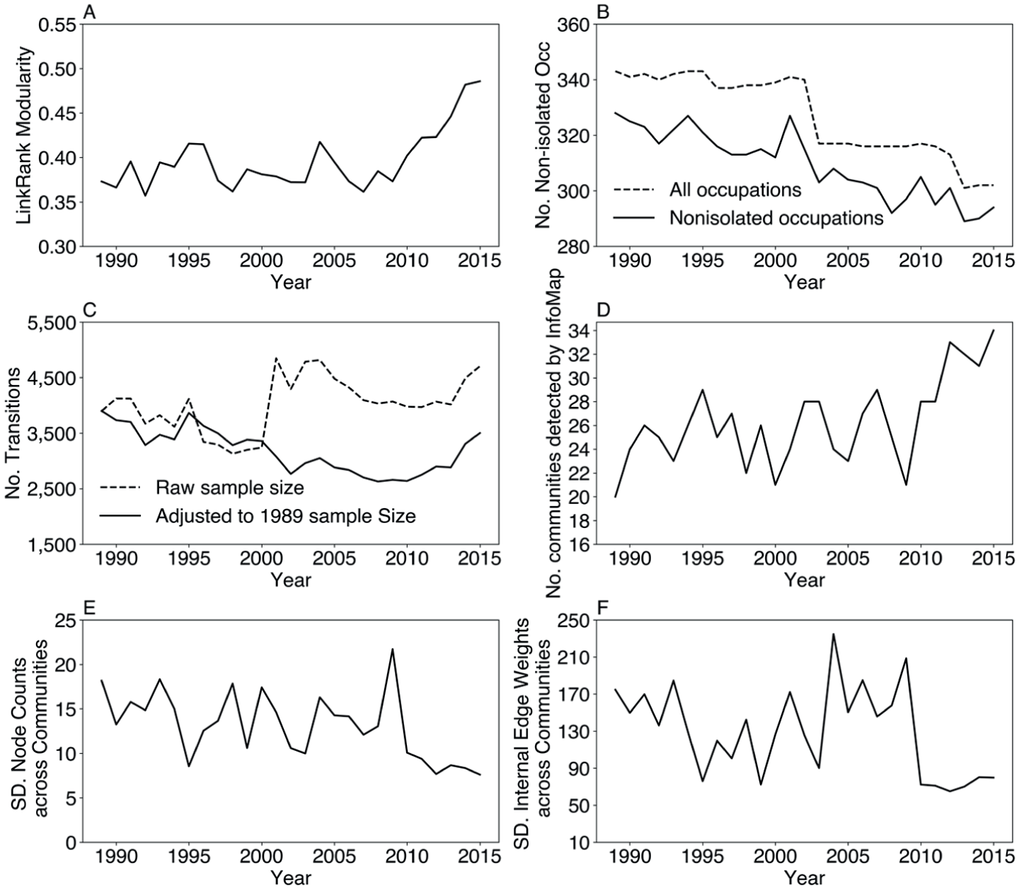
Replicating Cheng and Park (2020) and sample description.
Comparability Issues in This Case
Following the multistep framework, we evaluate the comparability issues in this case sequentially. First, regarding the choice of modularity metrics and conceptual alignment, Cheng and Park carefully chose a suitable modularity metric: LR modularity. This metric captures the directional and multistep moves, which are relevant to the concept of rigidity of mobility class boundaries. Cheng and Park also replicated their findings using GN modularity.
Second, regarding algorithm dependency, Cheng and Park were also thoughtful. They selected a non-modularity-based algorithm—the Infomap algorithm—to detect communities. Thus, they separated community detection from modularity calculation.
Third, regarding network dependency, there may be several major challenges. Figures 6B to 6F show substantial variations of several network characteristics from 1989 to 2015, particularly after 2009, when LR modularity rose rapidly (Figure 6A). Specifically, we see (1) a significant decline in the number of nonisolated nodes (Figure 6B), (2) a decline in the total edge weights before the mid-2000s and a subsequent increase (Figure 6C), (3) an increase in the number of communities detected by Infomap after 2009 (Figure 6D), and (4) a sharp homogenizing of community size since 2009, as reflected by the drop of standard deviation of the node and edge counts across detected communities (Figures 6E and 6F). On the basis of the systematic simulations presented in Figures 3 and 4 and Appendix A in the online supplement, these factors would exert potential biases to the findings and merit systematic considerations.
Cheng and Park did acknowledge the potential issues that could arise from (2) and (3). Regarding the change in total edge weights, Cheng and Park (2020:607) assigned yearly weights to all networks to make their edge weights the same as those in 1989. Regarding the rise in number of communities, Cheng and Park (2020:577, 604–606) interpreted this as showing an increase in labor market segmentation and the decoupling between job mobility boundaries and predefined classes. However, this reweighting strategy and interpretation essentially assume that community structures are robust to adding or removing edges. This assumption may be difficult to maintain in sparse networks (Botta and Del Genio 2016) like those in this case, in which small edge changes can alter detected partitions.
Fourth, regarding validation using nonmodularity measures, although Cheng and Park offer a series of substantively relevant analyses to enrich our understanding of the trend in U.S. labor market mobility, we believe supplementing nonmodularity measures in this case is still illustrative.
Reexamination of the LR Modularity Trend
The previous section reveals that network dependency and external validation require more attention in Cheng and Park’s study. Regarding network dependency, we follow our network standardization suggestions. First, we keep the common nodes (occupations) across all networks so they have the same set of nodes. Second, to account for the changing total edge weights (occupation transitions), we use bootstrapped standardization by randomly dropping the excessive occupational transitions such that the sum of edge weights is the minimum among all years. We repeated this standardization 100 times and present the findings in Figure 7.
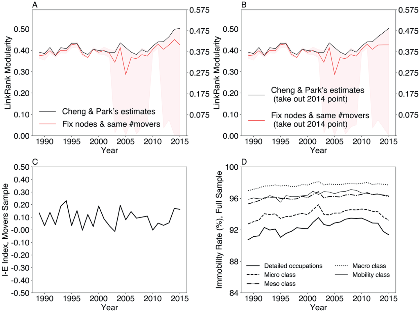
Results after network standardization and validation using nonmodularity measures.
In Figures 7A and 7B, the black lines replicate Cheng and Park’s (2020) LR modularity, and the red lines indicate the average LR modularity based on the 100 bootstrapped samples. 5 Figure 7A shows that, after bootstrap standardization, the rising trend persists but becomes much milder after the mid-2000s. Notably, the rise is driven mainly by the 2014 uptick, which has a large bootstrap CI. If we remove this 2014 outlier, the rising trend almost disappears (Figure 7B), suggesting almost no increase in the rigidity of mobility boundaries.
Regarding external validation, we use simpler and straightforward indicators to evaluate the evolution of labor market rigidity. First, we check the internal-external (I-E) index using Cheng and Park’s analytic sample, which keeps only movers across detailed occupations, with the communities detected by Infomap (Figure 7C). The I-E index is the additive inverse of the conventional E-I index. A higher I-E index reflects more rigid mobility class boundaries. As shown in Figure 7C, instead of describing the trend as increasing, it is more accurate to describe it as periodically fluctuating: the high value in 2014 is lower than the three peaks before 2005.
Second, we plot the temporal trends of immobility rates (the ratio of stayers) in the full sample for different occupation/class schemes, including the conventional macro-, meso-, and micro-class schemes, the mobility classes defined by Cheng and Park (2020), and the detailed occupations in the 1990 occupation scheme (Figure 7D). The macro-, meso-, and micro-class schemes are predefined occupational classifications that are time-invariant. Specifically, the macro-class scheme largely follows Erikson-Goldthorpe’s big-class tradition and contains five categories: professional-managerial, routine nonmanual, manual, primary, and military. The meso-class scheme (10 categories) follows the Featherman-Hauser approach, which provides a finer-grained hierarchy reflecting gradations in occupational status and prestige. The micro-class scheme adopts Jonsson et al.’s (2009) revision of Weeden and Grusky (2005), capturing detailed occupational distinctions (82 categories) that reveal the role of labor market closure and task specialization in shaping mobility. Cheng and Park (2020) made practical revisions to these schemes, and we adopt their revised version.
Substantively, higher immobility rates reflect more rigid class boundaries. As Figure 7D shows, the immobility rates for the macro-, meso-, and mobility classes were stable between 1989 and 2015, which disconfirms the post-2009 rising job class rigidity as estimated by Cheng and Park (2020), but aligns better with our standardized results that show stable modularity trends. Moreover, the immobility rates for micro-classes and detailed occupations have decreased since 2009, suggesting an increasing fluidity in the U.S. labor market since then.
In summary, these findings illustrate the importance of addressing network dependency and validation using nonmodularity measures. We recover a relatively stable trend out of a trend ending with a sudden rise, which aligns better with earlier works (e.g., Jarvis and Song 2017; Kambourov and Manovskii 2009). Cheng and Park (2020:626) explained the contradiction between the rising modularity based on mobility classes and the decreasing immobility rates for micro-classes and detailed occupations by emphasizing the difference between mobility classes and other class schemes. They summarized that while “micro-class boundaries have become more permeable over time,” the movements of workers were increasingly constrained by the mobility classes that crosscut the predefined micro-classes and detailed occupations. However, our findings suggest that even for mobility classes, the immobility rate in the full sample, the I-E index in the mover sample, and the adjusted LR modularity remain pretty stable over time, offering limited evidence for increasing mobility rigidity of the U.S. labor market.
Empirically Calibrated Simulations: If Not Increasing Rigidity, Why Rising LR Modularity?
Careful readers may notice that LR modularity still slightly increases after network standardization (Figures 7A and 7B), despite the I-E index and immobility rates (Figures 7C and 7D) being stable or even decreasing after 2009. The previous section demonstrated the importance of addressing network dependency, but we did not provide direct evidence regarding what, if not the increasing rigidity, drives the rising LR modularity.
It is worth noting that among the network attributes in Figure 6, our network standardization can only account for the temporal variation in node counts and edge weights: it cannot directly address the temporal variation in the number of communities (Figure 6D), the node distribution (Figure 6E), and the edge distribution (Figure 6F) across communities. Figure C1 in the online supplement shows significant temporal variation of these factors even after network standardization. Specifically, there were an increasing number of communities and equalizing node and edge distributions across communities after 2009. To evaluate the extent to which these temporal variations contribute to the rising LR modularity, we conducted a series of empirically calibrated simulations.
The calibrated simulations mimic the empirical networks in Cheng and Park (2020) by incorporating their networks’ observed characteristics into the parameters when generating the synthetic networks. These observed characteristics include the node set, community structure (i.e., community membership of nodes), total edge weights, community-level and node-level in-degree and out-degree marginal distribution, and the average probability of job transitions across communities (community-level I-E index). We predefine the communities in these simulated synthetic networks on the basis of the observed networks, and we use the community-level I-E index, which reflects the level of boundary rigidity, to guide our allocation of external and internal edges across communities. Using these synthetic networks, we present five sets of nested simulations in Figure 8 to evaluate the effects of variations in (1) community boundary rigidity (community-level I-E index), (2) number of communities, and (3) node and (4) edge distributions across communities on the LR modularity trends in this case. More technical details can be found in Appendix C in the online supplement and our replication package.
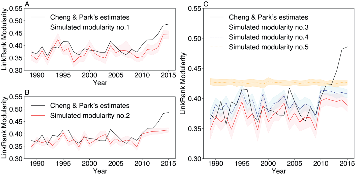
Empirically calibrated simulations to evaluate the effects of node and edge distributions.
Figure 8A, establishes the benchmark simulation, where all parameters follow their empirically observed patterns. The simulated modularity (red line) closely tracks Cheng and Park’s original estimates (black line), demonstrating that the experimental manipulations are operating on a credible representation of the empirical mobility networks.
Figure 8B introduces the first crucial constraint: fixing the community-level I-E index at the grand mean across all years (“simulated mobility no. 2”). If rising modularity primarily reflects genuine increases in boundary rigidity, the modularity should become flat. However, the simulated modularity continues to exhibit upward trends. This panel demonstrates that modularity can fluctuate substantially even when the underlying community boundary rigidity remains unchanged, suggesting that other structural factors are at play.
Figure 8C presents three additional sets of nested simulations to evaluate other structural factors. On the basis of the no. 2 simulation settings, no. 3 (the red solid line) fixes the number of communities at the minimum across all years; no. 4 (the blue dashed line) builds on no. 3 by equalizing node distribution across communities in all years; and no. 5 (the orange dotted line) builds on no. 4 by equalizing edge distribution across communities in all years. In the no. 3 simulated modularity, we see a disappearance of the uptick after 2009 but similar fluctuation patterns as in Figure 8B, indicating that changes in the number of communities cannot account for the entire fluctuation in the modularity trend. The no. 4 pattern is similar to no. 3, suggesting little effect of the node distribution. In contrast, the no. 5 simulated modularity becomes essentially flat, which pinpoints the key source of the spurious increase—shifting concentration of edges across communities.
Taken together, by progressively constraining different network parameters while allowing others to vary, these simulations reveal that rising modularity may emerge as an artifact of changing network attributes, rather than genuinely reflecting increasing boundary rigidity. In this case, the rising LR modularity is likely driven by the confounding effects from the increasing number of job changers since the late 2000s (Figure 6C), which split some big mobility communities and result in an increasing number of communities (Figure 6D) with more equalized edge distributions (Figure 6F).
Conclusion and Discussion
The emergence of computational social sciences has facilitated productive interdisciplinary exchange. The development of modularity metrics exemplifies this exchange. Girvan and Newman’s modularity framework (Girvan and Newman 2002; Newman and Girvan 2004) introduced technical innovations for analyzing large-scale networks by bridging social scientists’ long tradition of studying network structures (e.g., Breiger et al. 1975; Freeman 1978; Wasserman and Faust 1994; White et al. 1976) with developments in physics and computer science.
Recent years have seen further development in community detection methods, including artificial intelligence and deep learning approaches (for a comprehensive review, see Fortunato and Newman 2022). Here, we focus on the literature directly relevant to cross-network modularity comparison and its associated methodological challenges. This increasingly common but methodologically complex practice emerged primarily within the social sciences using established modularity metrics (i.e., GN and LR modularity). Although modularity could be effective in detecting community structures within networks, a purpose for which it was originally designed, this comparative approach requires careful considerations of concept mismatch, algorithm dependency, and network dependency issues.
Modularity is an expectation-adjusted comparison, with different modularity metrics using different null models for comparison. Hence, different modularity metrics’ variation across the same set of social networks can be different and align with different substantive concepts. Many studies provide clear theoretical justifications for their modularity choices, but additional consideration of concept alignment across networks can enhance the validity of findings.
We illustrated the algorithm and network dependency issues of this comparative approach and provided some empirical remedies. For algorithm dependency, in addition to existing strategies like conducting robustness checks with different community detection algorithms, we emphasize the importance of separating community detection from modularity estimation using non-modularity-based community detection algorithms. We also highlight recent advances in resolution-adjusted modularity. The challenge of this approach, however, concerns parameter selection, which remains an open question and merits careful consideration. For network dependency, we warn against the current strategy of simply rescaling or reweighting network size. Rather, we propose to use the recently developed network-robust modularity metrics if they can capture the concepts of interest. If, however, network-sensitive modularity metrics must be used, we show the effectiveness of fixing the common nodes and/or randomly dropping the excessive edges (or nodes) to standardize network sizes and estimate the bootstrap CIs of the modularity scores. It would also be useful to conduct robustness checks using nonmodularity metrics that capture the same concepts of interest. Only by doing so can scholars ensure the reliability and meaningfulness of their research findings.
Our reanalysis of Cheng and Park (2020) illustrates how the methodological framework we propose can be systematically applied in empirical research. This particular case focuses on occupational mobility, but the challenges we identify and the solutions we demonstrate apply broadly across substantive domains. Researchers studying scientific consensus through citation networks, political polarization through legislative co-sponsorship networks, or audience fragmentation through media networks all face similar comparability challenges. By presenting our methodological recommendations with an implementation framework, readers can easily adapt our method to their own research questions and network contexts. The value of this illustration lies not in revisiting debates about U.S. labor market mobility, but in demonstrating how careful attention to modularity comparability issues can alter substantive conclusions in empirical studies.
Last but not least, we note that our work focuses on the challenges of comparing modularity across already constructed networks. Appropriate network construction, however, is a crucial prerequisite for any meaningful modularity comparison. The question of how to define nodes and edges—including whether and how to assign edge weights or signs—represents a distinct and substantial methodological literature (for comprehensive reviews, see Borgatti et al. 2009; Marsden 1990). We do not address these network construction issues, assuming networks have already been appropriately constructed for the research question at hand. The challenges we identify arise even when networks are well-constructed, and poor network construction would compound these issues further. Therefore, careful attention to network construction should precede the modularity comparison procedures we recommend.
Supplemental Material
sj-docx-1-smx-10.1177_00811750261454676 – Supplemental material for Comparing Modularity Scores across Different Social Networks: Pitfalls, Illustrations, and Suggestions
Supplemental material, sj-docx-1-smx-10.1177_00811750261454676 for Comparing Modularity Scores across Different Social Networks: Pitfalls, Illustrations, and Suggestions by Ling Zhu, Ji Cao, Runhui Tian, Yujie Li, Xiaoqian Yue, Donghang Qi and Hai Liang in Sociological Methodology
Footnotes
Acknowledgements
We are grateful to the Computational Social Science Laboratory at the Chinese University of Hong Kong for supporting this research. We also benefited from the editors’ and anonymous reviewers’ comments, as well as comments from the participants at the 2023 Joint Workshop on Computational Social Sciences held at the Chinese University of Hong Kong, the 2024 Annual Meeting of the European Sociological Association, the 2025 Annual Meetings of the International Chinese Sociological Association, and the 2025 Annual Meetings of the International Sociological Association.
Authors’ Note
The authors declare that this study complies with required ethical standards. Artificial intelligence tools were used for grammar, proofreading, and clarity improvement only.
Funding
The authors disclosed receipt of the following financial support for the research, authorship, and/or publication of this article: This work was partly supported by the Research Grants Council of Hong Kong (ECS24621821, GRF14620122, and GRF14618523) and the Faculty of Social Science at the Chinese University of Hong Kong (4930984).
Declaration of Conflicting Interests
The authors declared no potential conflicts of interest with respect to the research, authorship, and/or publication of this article.
Data Availability Statement
Code for data analysis has been deposited at the Open Science Framework (https://osf.io/w9vs7/). Anonymized Current Population Survey Annual Social and Economic Supplement data are deposited at IPUMS (![]() ).
).
Supplemental material
Supplemental material for this article is available online.
Notes
Author Biographies
References
Supplementary Material
Please find the following supplemental material available below.
For Open Access articles published under a Creative Commons License, all supplemental material carries the same license as the article it is associated with.
For non-Open Access articles published, all supplemental material carries a non-exclusive license, and permission requests for re-use of supplemental material or any part of supplemental material shall be sent directly to the copyright owner as specified in the copyright notice associated with the article.