Causal Inference with a Continuous Treatment: Addressing Positivity Constraints,Nonlinearity,and Effect Heterogeneity

Abstract

Causal inference approaches often emphasize binary treatments. But in many applications, the underlying constructs are continuous. In the potential outcomes framework, a continuous treatment can take on numerous values, each corresponding to a potential outcome that may be realized. In this setting, common estimands may be intractable because of a common issue in social research, particularly research on social inequality: the exposure is highly stratified by confounders. The authors show how to avoid drawing inferences about counterfactuals where data are unlikely to exist by carefully selecting the causal estimand. The authors adopt an additive shift estimand that adds a small, fixed amount to each unit’s income. This approach is preferable to population-average dose-response curves in settings in which some treatment values rarely occur in some subgroups. The authors also show how to estimate and summarize patterns of nonlinearity and effect heterogeneity with continuous treatments. As a motivating example, the authors consider the causal effect of parental income on college attendance, a setting in which the exposure is highly stratified by confounders (e.g., parental education). This approach applies to a wide range of possible treatment conditions in sociology.

Keywords

causal inference continuous treatment effect heterogeneity nonlinear effect inequality social stratification

The widespread adoption of causal goals has unlocked new understandings in social research. Drawing inspiration from randomized controlled trials, many such studies begin by defining one treatment condition and one control condition. For example, people who completed a four-year college degree (a treatment condition) may not have completed that degree (a control condition). By studying the socioeconomic outcomes that would have resulted under each treatment assignment, scholars have gained new understandings of the causal role that college degrees can play in improving outcomes and breaking intergenerational cycles of disadvantage (Brand 2023; Brand and Xie 2010; Zhou 2024). As an example of an estimator in this framework, some researchers match treated units to comparable untreated units who serve as estimates for the counterfactual outcomes the treated units would have realized in the absence of treatment (Rosenbaum 2010; Stuart 2010).

Yet many causal inputs are continuous rather than binary. A child’s life chances might be shaped by the numeric value of their family’s income, their school’s student-teacher ratio, or their neighborhood’s homicide rate. Instead of two potential outcomes, each person has many: one for each value the numeric treatment could take (see Figure 1). Whether the treatment is truly continuous, with an infinite number of possible values, or discretely numeric, with a large but finite number of values, numeric treatments yield many potential outcomes. Just as randomized controlled trials motivated causal claims with binary treatments, an analogous (albeit rarely used) experimental design can motivate causal claims with continuous treatments. Imagine a cash transfer program in which the amount of cash transferred to recipients is drawn uniformly at random over some range. Researchers could measure each recipient’s outcome and then estimate a smooth curve to summarize the average response to various values of the treatment. This causal research goal, known as the average dose-response curve, is one example from a broad literature in statistics that generalizes causal inference from binary treatments to continuous exposures in both randomized and observational settings (Díaz and van der Laan 2013; Gill and Robins 2001; Hirano and Imbens 2004; Imai and Van Dyk 2004; Kennedy et al. 2017; Rothenhäusler and Yu 2019; Takatsu and Westling 2025).

Figure 1.

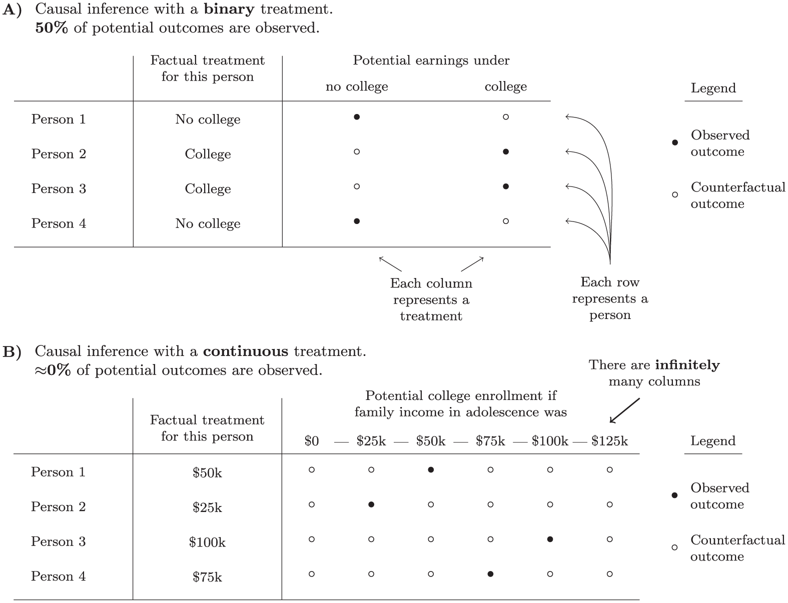
A continuous treatment creates infinite potential outcomes. (A) Causal inference with a binary treatment. Fifty percent of potential outcomes are observed. (B) Causal inference with a continuous treatment. Approximately 0 percent of potential outcomes are observed.

Our contribution is applied: we demonstrate how sociologists can apply causal approaches with continuous exposures. Although we draw heavily on existing statistical approaches, we argue that the population-average dose-response curve is often intractable for the types of questions commonly studied in sociology, where an input of interest (e.g., family income) is itself strongly shaped by measured confounders (e.g., parental education). We also demonstrate how two concepts, effect heterogeneity and nonlinearity, become empirically intertwined in settings in which measured confounders strongly shape treatment values. We show how a pivot to a different research goal, the additive shift estimand, avoids the problem of making counterfactual estimates far from the data. Our approach produces interpretable causal estimates even in settings in which measured confounders strongly influence treatment values.

Causal Effects of a Continuous Treatment

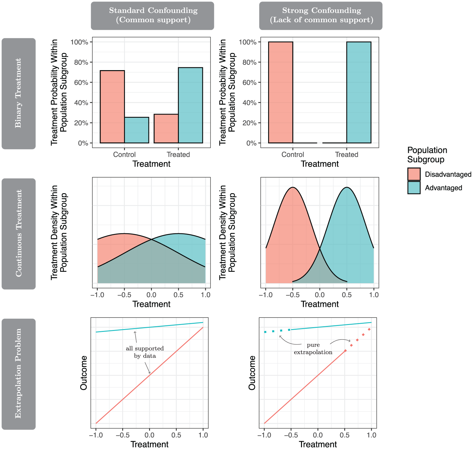
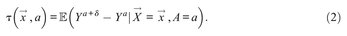
When evaluating the causal effect of a continuous treatment $A$ on an outcome $Y$ , social scientists often begin by measuring many confounding variables $\vec{X}$ and then estimating a linear regression model.

Researchers then interpret $β$ as the increase in the outcome $Y$ that would result from a unit increase in the continuous treatment $A$ . This additive regression is simpler than many regressions used in practice, but its simplicity will allow us to illustrate connections to causal inference approaches as well as some serious problems that arise.

From a statistical standpoint, this regression model can be interpreted as an estimator of a causal dose-response curve. Here we spell out the connection, which is useful for seeing additive ordinary least squares regression as a particular example within a broader class of possible estimators. For each unit $i$ , define $Y_{i}^{a}$ as the potential outcome that would be realized if unit $i$ were exposed to treatment value $A_{i} = a$ . Taking the average over units and drawing a curve through treatment values $a$ yields the causal dose-response curve $E (Y^{a})$ , which captures the average value of the outcome as a function of the treatment value $a$ . In this hypothetical curve, we are imagining the same set of people (with the same distribution of pretreatment covariates $\vec{X}$ ) summarized at every possible treatment value $a$ . But in observational data, the covariate vector $\vec{X}$ tends to be different among those at different values of the treatment variable $A$ . The regression model can be understood as a strategy to address this problem: by controlling for $\vec{X}$ , the researcher can learn the curve by which $A$ is associated with $Y$ , given a particular value of $\vec{X}$ .

Three steps are implicit in the regression strategy. First is a causal identification step: the researcher must assume $\vec{X}$ is a sufficient adjustment set to block confounding, so the mean outcome $E (Y ∣ A = a, \vec{X} = \vec{x})$ among those with treatment value $A = a$ and confounder vector $\vec{X} = \vec{x}$ is equal to the mean among all people with this confounder vector if hypothetically assigned to that treatment value, $E (Y^{a} ∣ \vec{X} = \vec{x})$ . Second is a parametric regression step: the researcher assumes the conditional mean $E (Y ∣ A = a, \vec{X} = \vec{x})$ follows the particular functional form of a regression model, such as equation (1). Third is a prediction step: the researcher uses the estimated regression model to predict the dose-response curve. To predict the outcome $E (Y^{a})$ , the researcher first assigns all respondents to the treatment value $A = a$ while leaving their pretreatment covariates at $\vec{X} = {\vec{x}}_{i}$ . The researcher then predicts their conditional mean outcome $\hat{E} (Y ∣ A = a, \vec{X} = {\vec{x}}_{i})$ . Finally, they marginalize over the population distribution of $\vec{X}$ by taking the sample average of the predicted values, weighted by sampling weights $w_{i}$ if the sample is an unequal probability sample. The estimate is $\hat{E} (Y^{a}) = \frac{1}{\sum_{i} w_{i}} \sum_{i} w_{i} \hat{E} (Y ∣ A = a, \vec{X} = {\vec{x}}_{i})$ .

In the additive ordinary least squares model of equation (1), the predicted conditional mean outcome for unit $i$ under treatment value $a$ is $\hat{α} + a \hat{β} + {\vec{x}}_{i}' \hat{\vec{γ}}$ . The average simplifies to the form $\hat{E} (Y^{a}) = \hat{α} + a \hat{β} + {\bar{\vec{X}}}^{'} \hat{\vec{γ}}$ , where $\bar{\vec{X}}$ is the weighted sample mean of the pretreatment covariate vector. By comparing the predicted value at treatment $a$ and $a + 1$ , we see that the coefficient estimate $\hat{β}$ has the commonly understood interpretation: the estimated change in $Y$ that would result from a causal intervention to increase the treatment $A$ by one unit. This particular case is useful for building intuition, but we will highlight several key limitations of this regression approach. We ultimately advocate a related but distinct approach, involving a different causal estimand and a more flexible regression specification.

Effect Heterogeneity and Nonlinearity: Why $β$ Is an Inadequate Causal Estimand

The main problem with a $β$ -centric approach to causal inference is that this approach relies on two key parametric assumptions. First, an effect homogeneity assumption implicit in equation (1) is the absence of interactions between treatment $A$ and covariates $\vec{X}$ , so that the effect of a change in treatment is assumed to be the same in every population subgroup. Second, a linearity assumption implicit in equation (1) is that any unit change in treatment $A$ produces the same change in outcome $Y$ regardless of the initial value of the treatment. This assumption may be doubtful, for example, in settings with diminishing returns to treatment. When these assumptions do not hold, a model based on them can be misleading and extrapolate in troubling ways, as we show below. A more credible approach would allow the world to be characterized by two patterns not captured by the regression coefficient: effect heterogeneity and nonlinearity.

Scholars of causal inference widely agree that the same causal intervention is likely to have different average effects in distinct population subgroups (Brand, Zhou, and Xie 2023; Smith 2022; Xie 2013). Rather than simply asking whether a causal effect is large on average, we should also ask for whom the effect is largest. The search for effect heterogeneity has led to numerous advances. One example is evidence that completion of a four-year degree is most beneficial for graduates from the most disadvantaged social origins (Brand 2023; Brand and Xie 2010; Cheng et al. 2021; Hout 1988, 2012; Torche 2011). These findings have led to new insights in sociology and public policy, informing debates about how educational expansion can equalize opportunities across individuals from different backgrounds (Witteveen and Attewell 2020; Zhou 2019).

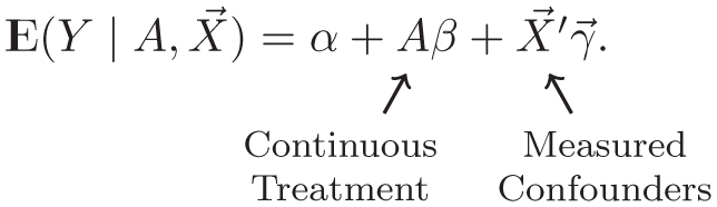
When the treatment is continuous, the concept of effect heterogeneity generalizes to two axes of variation: nonlinear effects of treatment $A$ and heterogeneous effects of treatment $A$ across pretreatment population subgroups defined by $\vec{X}$ (see Figure 2). A regression such as equation (1) works well in the linear, homogeneous setting illustrated by the two parallel lines in the top left of Figure 2. A unit change in treatment $A$ increases outcome $Y$ by the same amount $β$ regardless of the initial value of the treatment. But in many settings, response may be a nonlinear function of treatment $A$ . For example, we may observe diminishing returns such that a unit increase in $A$ leads to a smaller increase in $Y$ when the initial value of $A$ is larger (Figure 2, top right). Unless the nonlinearity is captured by a simple functional form such as the log, it is difficult to summarize a nonlinear curve by a single regression coefficient. Likewise, in either the linear or nonlinear setting, there may be effect heterogeneity: the pattern by which treatment $A$ causes outcome $Y$ may differ across subgroups defined by a pretreatment variable $X$ (Figure 2, bottom row).

Figure 2.

Nonlinear and heterogeneous effects are conceptually distinct.

Causal estimands in the potential outcomes approach are well defined regardless of whether effects are nonlinear, heterogeneous, or both. One can conceptualize the mean outcome, $E (Y^{a})$ , under a particular treatment value, a, without making any assumptions about functional forms. One can study effect heterogeneity by studying the expected value of potential outcomes under different subgroups, such as $E (Y^{a} ∣ X = x)$ and $E (Y^{a} ∣ X = x^{'})$ for two values $x$ and $x^{'}$ of a pretreatment variable $X$ . Furthermore, these estimands can be estimated using regression to predict potential outcomes, as in equation (1), or by more complex models that incorporate nonlinearity and effect heterogeneity.

The Extrapolation Problem

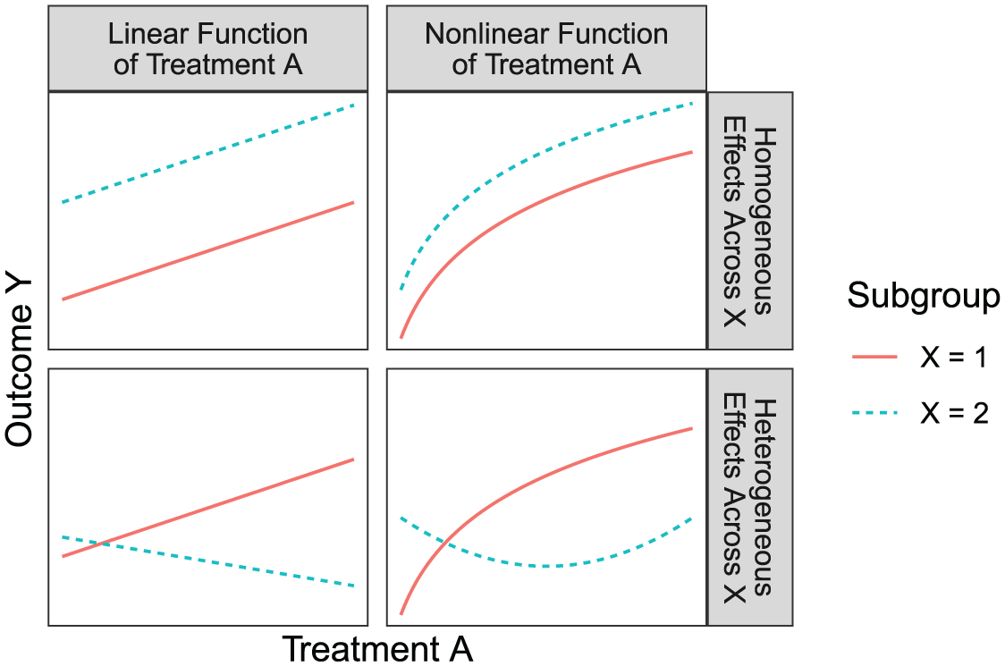
Nonlinearity and effect heterogeneity pose particular challenges in a setting common to sociological research: questions that require extrapolation beyond the support of the observed data. Under the assumptions of a linear model, such extrapolation appears straightforward; once those assumptions are relaxed, however, it may no longer be feasible. Figure 3 illustrates this through a hypothetical example in which two population subgroups (advantaged and disadvantaged) experience highly unequal exposure to a treatment variable.

Figure 3.

Strong confounding and the extrapolation problem.

The first row of Figure 3 considers a binary treatment. The panel on the left depicts standard confounding: the advantaged subgroup is assigned to treatment with a higher probability than the disadvantaged group, but a nonzero proportion of both groups is observed in the treatment and in the control condition. If the population subgroup were the only confounder, one could draw inferences by comparing across treatment conditions within population subgroups. The panel on the right shows the more difficult scenario of strong confounding: all units within the advantaged subgroup are treated, whereas all units within the disadvantaged subgroup are untreated. This setting is known as a lack of common support because the data cannot support causal inference: no one in the disadvantaged subgroup is exposed to treatment, and no one in the advantaged subgroup is exposed to the control.

A lack of common support poses similar risks when the treatment is continuous, yet it can be more difficult to recognize. With a binary treatment $A$ , a subgroup defined by $\vec{X}$ may exist in which both treatment values are observed. But with a continuous treatment $A$ , no subgroup can contain the full range of possible treatment values. Instead, one must consider the conditional distribution of the continuous treatment and how it compares across subgroups. The middle row of Figure 3 shows hypothetical distributions of a continuous treatment within the two population subgroups. On the left, all treatment values occur with nonzero density in both subgroups. On the right, the probability density function for treatment is zero for low treatment values in the advantaged subgroup and zero for high treatment values in the disadvantaged subgroup. Just as in the binary case, the data cannot yield credible inference about the potential outcomes of disadvantaged individuals under high treatment values, as these values never occur in that subgroup.

Linear regression estimators appear deceptively simple in this setting (Figure 3, row 3). In the standard confounding setting on the left, one might summarize how the outcome responds to the continuous treatment by a linear regression estimated separately within each population subgroup. Although this approach assumes a line, at least the data provide evidence about that line across the full treatment distribution. In the strong confounding setting on the right, a researcher might similarly estimate linear regression models within each subgroup. The researcher might then predict counterfactual outcomes at any treatment value, even the treatment values that represent pure extrapolation.

Extrapolation is often a problem in empirical social research. We used linear regression here, but extrapolation can be a danger with any estimator when the target of inference is far from where the data exist. Researchers using a causal inference framework with binary treatments regularly take steps to avoid extrapolation (i.e., restrict to the region of common support). But with continuous treatments, the problem of common support is rarely discussed. One possible reason for this discrepancy is that studies with continuous treatments often begin by assuming a linear model. Under the assumptions of that model, any counterfactual can be predicted even if that prediction involves extrapolation. But if the true effects are nonlinear and heterogeneous, then extrapolated predictions are not credible. We avoid this problem by defining a causal estimand with minimal extrapolation before making any modeling assumptions.

Credible Counterfactuals: Additive Shift Estimands

With a binary treatment, a solution to the lack of common support is to restrict to a region of support, which entails a change to the target population. With a continuous treatment, an alternative approach is possible: in each population subgroup, restrict counterfactual predictions to the range of treatment values with nonzero density. We advocate a causal estimand that is easy to interpret and, in many settings, avoids the extrapolation problem by focusing on a carefully chosen counterfactual treatment value.

To fix ideas, we illustrate this estimand using our motivating example, in which the treatment is family income and the outcome is college enrollment. Suppose child $i$ had a parental income of $60,000, and we observe whether that child enrolled in college $Y_{i}^{$ 60, 000}$ . Their parental income could hypothetically have been $70,000, in which case they would have realized the counterfactual outcome $Y_{i}^{$ 70, 000}$ . Because the increment $δ = $ 10, 000$ is small, this counterfactual treatment value would likely occur with nonzero density among children with the confounder values $\vec{X} = {\vec{x}}_{i}$ for unit $i$ . Perhaps child $i$ has two parents whose highest education was a high school degree. Other children whose parents had this level of education could reasonably have had family incomes of $70,000.

Formally, let $τ (\vec{x}, a)$ be the average causal effect of increasing $A$ by the additive shift $δ$ within the population subgroup with $\vec{X} = \vec{x}$ who factually have treatment value $A = a$ .

τ (\vec{x}, a) = E (Y^{a + δ} - Y^{a} ∣ \vec{X} = \vec{x}, A = a) .

(2)

The key benefit of an additive shift estimand is that it does not involve highly unlikely counterfactuals (as long as $δ$ is small). If child $i$ has two high school–educated parents, it is likely difficult to infer their counterfactual outcome if their parents’ income had been $1 million. By asking a causal question about a counterfactual treatment value that is a reasonable value $δ$ away from the factual treatment value, we focus on causal quantities unlikely to involve severe extrapolation.

One could in theory use an additive shift estimand for grander questions, where the value of $δ$ is large. For example, an intervention might shift low-income children’s family incomes by such a large amount they would become high-income. That research goal could be described by equation (2), with a large $δ$ . But the greater the value of $δ$ , the greater the risk of extrapolation and the more tenuous the resulting claims. We therefore focus on applications where the value of $δ$ is relatively small.

Identification and Estimation for Additive Shift Estimands

Standard assumptions for causal identification in binary settings apply to the continuous setting (Gill and Robins 2001; Robins 1987). Adopting terminology and notation following the conventions in Hernán and Robins (2021), we first assume that potential outcomes are well defined so that for each unit $i$ the observed outcome $Y_{i}$ equals the potential outcome $Y_{i}^{A_{i}}$ under the observed treatment $A_{i}$ .¹

\begin{matrix} Y_{i} = Y_{i}^{A_{i}} for all i & (consistency) \end{matrix} .

(3)

Considerations affecting the credibility of the consistency assumption are the same for both continuous and binary treatments. For example, in both cases, the assumption we defined above requires no interference such that unit $i$ ’s outcome does not depend on unit $j$ ’s treatment value. In both cases, the assumption requires no hidden versions of the treatment that lead to distinct potential outcomes (VanderWeele and Hernán 2013). A researcher who began with a continuous treatment but binned it into two categories for analysis would undermine the latter requirement; this is one reason it can be important to study continuous treatments as continuous rather than in coarsened form.

Second, we make a conditional exchangeability assumption defined for each unit $i$ . We assume that across all units with confounder vector $\vec{X} = {\vec{x}}_{i}$ , whether the treatment variable $A$ takes the value $A_{i}$ or counterfactual value $A_{i} + δ$ is independent of the potential outcome under this counterfactual value.

\begin{matrix} Y^{A_{i} + δ} ╨ A ∣ \vec{X} = {\vec{x}}_{i}, A \in {A_{i}, A_{i} + δ} for all i & (conditional exchangeability) \end{matrix},

(4)

where in our example $δ = $ 10, 000$ , and the confounding variables $\vec{X}$ include race, parental education, and parental wealth (see details in the section “Empirical Example: Effect of Parental Income on College Enrollment”). One can defend the conditional exchangeability assumption by drawing a Directed Acyclic Graph (Pearl 2009) in which the measured confounders $\vec{X}$ block all noncausal paths between the treatment and outcome. An implication of this assumption is an equality of conditional means, which is the minimally sufficient version of the assumption for identification.

\begin{matrix} \underset{\begin{matrix} Conditional mean \\ potential outcome \end{matrix}}{\underset{︸}{E (Y^{a + δ} ∣ A = a, \vec{X} = \vec{x})}} = \underset{\begin{matrix} Conditional mean \\ factual outcome \end{matrix}}{\underset{︸}{E (Y ∣ A = a + δ, \vec{X} = \vec{x})}} \end{matrix} .

(5)

In words, among units with treatment value $a$ and confounder vector $\vec{x}$ , the mean outcome under the counterfactual treatment value $a + δ$ equals the mean factual outcome among units who factually experience the treatment value $a + δ$ while sharing the confounder vector $\vec{x}$ .

The conditional exchangeability assumption implicitly requires a positivity assumption,

f_{A ∣ \vec{X} = {\vec{x}}_{i}} (A_{i} + δ) > 0 for all i (positivity),

(6)

that the conditional density of treatment value $A_{i} + δ$ is nonzero among the population with the covariate values $\vec{X} = {\vec{x}}_{i}$ of unit $i$ .² Without this assumption, the conditional distribution of $Y^{A_{i} + δ}$ in equation (4) would not be well-defined. This positivity assumption required for an additive shift estimand is much weaker than the corresponding positivity assumption required for a population-average dose-response curve, which would be that the conditional density of every possible treatment value $a \in support (A)$ is nonzero in every subgroup defined by $\vec{X}$ . A key advantage of additive shift estimands is that the required positivity assumption is credible.

Finally, we assume a statistical model for the conditional mean outcome given the continuous treatment $A$ and confounders $\vec{X}$ . We represent this model by a function $μ$ .

μ (\vec{x}, a) \overset{\begin{matrix} by assumed \\ model \end{matrix}}{\overset{︷}{=}} E (Y ∣ \vec{X} = \vec{x}, A = a) .

(7)

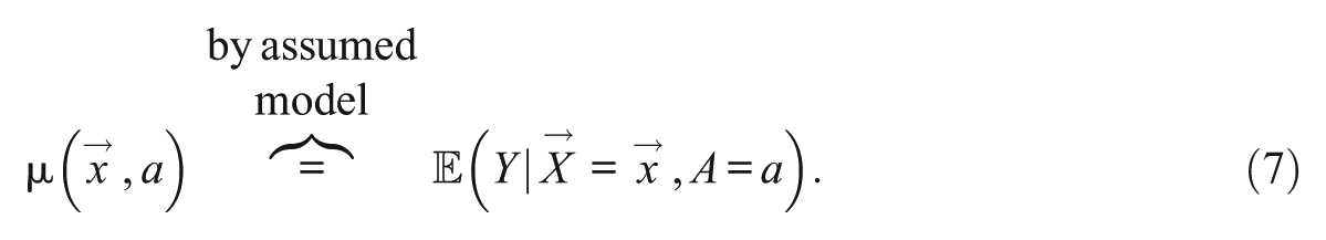
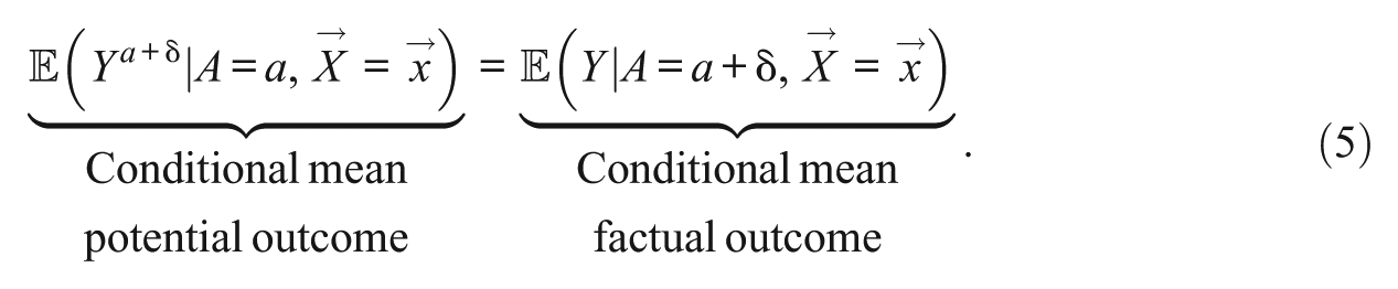
We then identify the additive shift estimand by a difference in conditional means under the incremented and nonincremented treatment values.

τ (\vec{x}, a) = μ (\vec{x}, a + δ) - μ (\vec{x}, a)

(8)

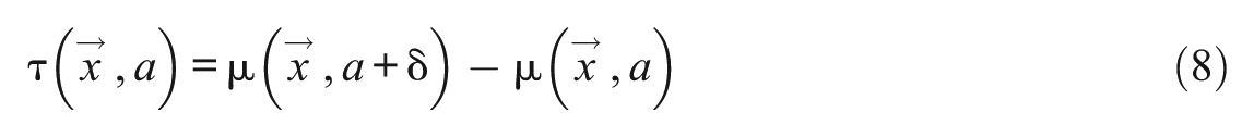
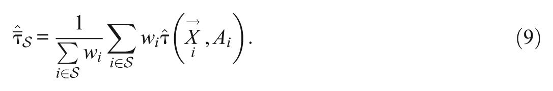
We may want to estimate the average value of the additive shift estimand within a subgroup $S$ of units with a particular range of treatment or covariate values. Assuming the sample is a probability sample with sampling weights $w_{i}$ , we estimate the average value of the additive shift estimand by the weighted sample mean of unit-specific estimates.

{\hat{\bar{τ}}}_{S} = \frac{1}{\sum_{i \in S} w_{i}} \sum_{i \in S} w_{i} \hat{τ} (X_{i}^{\to}, A_{i}) .

(9)

Because our procedure involves several steps (estimation and aggregation), we conduct statistical inference using a nonparametric bootstrap with 1,000 draws. We construct confidence intervals by a normal approximation using the point estimate and bootstrap estimate of the standard error.

Connections to Literature in Statistics

An additive shift estimand is one example of a broader class of estimands known as modified treatment policies, in which the counterfactual treatment value may depend on both pretreatment variables and the factual treatment value. An example is the causal effect of reducing the factual duration of a surgery by five minutes (Haneuse and Rotnitzky 2013). A modified treatment policy is conceptually distinct from a stochastic estimand, in which the counterfactual treatment value depends on pretreatment variables but not on the realized treatment value (Díaz Muñoz and van der Laan 2012). However, the two have many similarities. For example, a stochastic intervention assignment rule can be defined so that only realistic treatment values are assigned (Moore et al. 2012; Van der Laan and Petersen 2007), which is also our goal with additive shift estimands. A stochastic intervention can also be defined so that the statistical estimand is identical to that of a modified treatment policy (Haneuse and Rotnitzky 2013; Young, Hernán, and Robins 2014). For example, the modified treatment policy “increase the treatment value $A$ to $A + δ$ ” yields the same statistical estimand as the stochastic intervention “for each unit with covariate vector $\vec{x}$ , select a treatment value from the observed distribution $A ∣ \vec{X} = \vec{x}$ and increment that value by $δ$ .” The former is a function of the focal unit’s treatment value, whereas the latter is only a function of that unit’s pretreatment covariates. Both lead to the same statistical estimand and estimator. The difference is one of interpretation, and we follow the modified treatment policy interpretation in this article.

Additive shift estimands are a discrete version of the incremental causal effects studied by Rothenhäusler and Yu (2019), in which the estimand is the rate of change in the outcome per an infinitesimal increment to each unit’s treatment. Incremental causal effects are thus defined as the average value of a derivative, and are identified by statistical estimands equivalent to average partial effects that are already common in social science (Long 1997; Powell, Stock, and Stoker 1989; Wooldridge 2005). Yet estimands defined in terms of derivatives may be difficult to convey to broader audiences, such as the public and policymakers. We therefore choose to study the causal effect of discrete additive shifts that may be easier to interpret.

Our estimator of an additive shift estimand is equivalent to a common practice for interpreting nonlinear models through predicted values: predict under a factual value, predict after incrementing a chosen predictor, and summarize the differences. This procedure is the same as one might use in noncausal settings to summarize a logistic regression model by predicted probabilities under a discrete change (Hanmer and Ozan Kalkan 2013; King, Tomz, and Wittenberg 2000; Long and Mustillo 2021; Mize 2019; Mize, Doan, and Long 2019). But an additive shift estimand differs from a marginal effect because it involves an explicitly causal goal: the causal effect of increasing a particular treatment variable by a given amount.

We focus on outcome modeling, but an alternative strategy is to build a statistical model for the conditional treatment density $f (A ∣ \vec{X})$ and then proceed using inverse density weighting, marginal structural modeling, or doubly robust estimation. We chose outcome modeling because we find it more intuitive to reason about models for the conditional mean of an outcome than the conditional density of a continuous treatment. Models for conditional means may also be more familiar to many social scientists. This choice simplifies the researcher’s task at some cost to asymptotic efficiency (see Díaz and van der Laan 2018; Haneuse and Rotnitzky 2013).

Summary: Why Use Additive Shift Estimands

Linear regression models such as equation (1) are by far the most common approach to continuous treatment variables in the social sciences. Yet the specification of these models raises immediate concerns. First, how should one conceptualize the summary coefficient $β$ if the true effects are nonlinear or heterogeneous (Figure 2)? Second, the regression approach does not motivate defining the research goal within the potential outcomes framework, thereby forgoing the opportunity to draw on well-established causal reasoning for binary treatments. By adopting additive shift estimands, researchers gain the clarity of the potential outcomes framework without confronting an infinite set of potential outcomes (see Figure 1). Instead, each unit has only two relevant potential outcomes, one observed and one unobserved, analogous to the conceptual apparatus for causal inference for binary treatments (Holland 1986). Finally, additive shift estimands empower researchers to explore nonlinear and heterogeneous effects using methods analogous to those we use to study effect heterogeneity with binary treatments.

Empirical Example: Effect of Parental Income on College Enrollment

We demonstrate causal identification assumptions and estimation approaches through an empirical illustration of the causal effect of parental income on college enrollment. Family income is a powerful indicator of socioeconomic advantage. Children from high-income families are more likely to enroll in and complete college (Acemoglu and Pischke 2001; Bailey and Dynarski 2011; Belley and Lochner 2007; Bloome, Dyer, and Zhou 2018; Voss, Hout, and George 2024) and earn more as adults (Chetty et al. 2014). In addition to descriptively marking life chances, family income may also cause life chances. Income enables parents to purchase goods that facilitate children’s success in school, such as nutritious food, medical care, academic enrichment activities, and homes in neighborhoods with high-quality schools (Bloome et al. 2018; Duncan and Murnane 2011; Farkas 2018; Kornrich 2016; Kornrich and Furstenberg 2013; Reardon 2011; Schneider, Hastings, and LaBriola 2018; Voss et al. 2024). Increasing income inequality has also meant growing class gaps in investments that affect children’s education (Reardon 2011). Among college enrollees, low-income students often lack economic resources and face barriers to completion (Goldrick-Rab et al. 2016; Houle 2014; Jack 2019; Regan 2020). Whereas prior causal work on the effect of family income has focused on the problem of unmeasured confounding (Elwert and Pfeffer 2022; Mayer 1997), we focus on the more tractable problem of measured confounding and show how additive shift estimands can yield improved estimates.

Data

We analyze data from the National Longitudinal Survey of Youth 1997 cohort (NLSY97). The NLSY97 began with a probability sample of U.S. youths 12 to 17 years of age in 1997 followed across repeated interviews through 2019. From the original sample of 8,984 respondents, we make several sample restrictions. We first restrict to the 6,588 youth with valid reports of our treatment variable: total gross household income in 1996 as reported in the 1997 survey wave when respondents were ages 12 to 17. We adjust to 2022 dollars using the Consumer Price Index and bottom-code at $10,000. The NLSY97 top-codes 1996 family incomes at the top 2 percent ($449,299 in 2022 dollars). We restrict to the 6,455 respondents with incomes below this survey-enforced top code, because the data are uninformative about the effects of income changes above this value. We measure enrollment as any report of enrollment in any college up to age 21. We restrict to the 6,357 respondents who either reported college enrollment before age 21 or were observed at ages 19 to 21 but reported no college enrollment.

We measure three confounding variables: race, parents’ education, and wealth. Race is categorized as Hispanic, non-Hispanic Black, and non-Hispanic White or other, as coded in the 1997 survey. We refer to these categories as Hispanic, Black, and White or other. Parents’ education is measured as no parent completed college, one parent completed college, or two parents completed college. We constructed this variable from reports by the residential mother and father in 1997. The variable implicitly indicates family structure; a child with only one residential parent is always coded as either no parent completed college or one parent completed college. We chose this simple operationalization because we treat family structure as influencing children’s education insofar as it shapes whether children have access to one or more parents who understand the higher education system, and insofar as households with two college-educated adults are likely to have higher incomes. Wealth is the log household net worth reported by the parent in 1997, adjusted to 2022 dollars and bottom-coded at $10,000. Our models also include indicators for whether wealth before bottom-coding was (1) negative or (2) between $ 0 and $10,000.

Adjusting for only three confounding variables simplifies our methodological illustration. In this setting, our causal identifying assumptions (see the section “Identification and Estimation for Additive Shift Estimands”) are likely to be violated to some degree. Yet our main claim is that positivity violations are serious and require a change in how researchers define their estimand. These positivity violations would be even more severe if our confounder set included a richer set of variables that might shape family income. We thus take our analysis using three confounding variables as a conservative illustration of a problem that is likely to be even more serious in applications with a larger set of confounders.

Hypotheses

Additive shift estimands enable us to generate hypotheses about heterogeneous effects, analogous to those generated for binary treatments. In our setting, we expect nonlinear effects of family income. Because of diminishing returns, a fixed increase in income may be less consequential for youth in families with already high incomes. We therefore expect differences in treatment effects across subpopulations defined by the baseline treatment value.

Hypothesis 1: An increase in family income would more strongly affect college enrollment among youth with low parental income.

We also expect effect heterogeneity by selected confounders. By a logic similar to that in hypothesis 1, a small increase in family income may be more consequential for youth in families with lower wealth.

Hypothesis 2: An increase in family income would more strongly affect college enrollment among youth with low parental wealth.

Finally, parental education is a key, if not the most important, factor affecting children’s educational attainment. The overwhelming majority of youth whose parents hold bachelor’s degrees enroll in postsecondary education (Chen et al. 2017). College-educated parents support and advise their children in college selection, preparation, application, and financial aid processes, whereas less educated parents have limited resources to help their children navigate higher education (Hout and Janus 2011). More educated parents also spend an increasingly large amount of time on developmental activities that cultivate educational achievement (Lareau 2003). Youth with more educated parents, who have a very high likelihood of college enrollment, could therefore be less sensitive to incremental increases in family income. By contrast, for children who might otherwise not attend college because of low parental education, an increase in parental income could be more consequential for attaining higher levels of education.

Hypothesis 3: An increase in family income would more strongly affect college enrollment among youth whose parents did not complete college.

Identification and Estimation

In our empirical example, our consistency assumption is that each child’s college enrollment equals the enrollment they would realize if hypothetically exposed to an intervention to set their family income to the value that actually occurred for that child ( $Y_{i} = Y_{i}^{A_{i}}$ ). The conditional exchangeability assumption is that family income is independent of the potential outcome that would have been realized if income had been $10,000 higher, conditional on race, wealth, and parental education. This assumption holds in the directed acyclic graph in Figure 4 (excluding the red node and edges), where this set blocks all noncausal paths between family income $A$ and college enrollment $Y$ . Unobserved confounding would threaten our estimates only to the degree that the unmeasured paths that create confounding are not blocked by our measured adjustment set. In the U.S. context, many likely unobserved confounders may be strongly related to race, parents’ education, and wealth because stratification processes are highly correlated. We therefore believe that adjustment for race, parental education, and wealth is an important step toward causal understanding, limitations notwithstanding.

Figure 4.

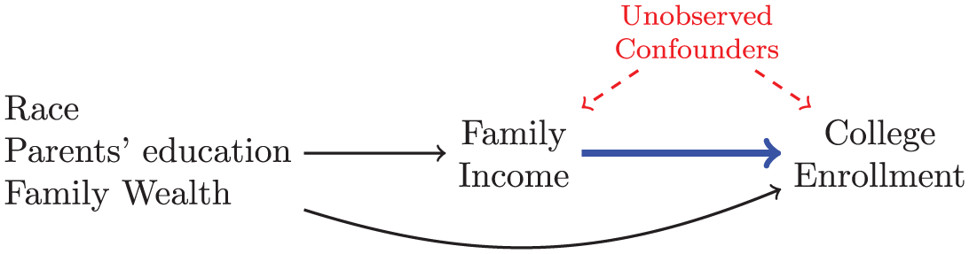
Causal assumptions in a directed acyclic graph.

We first estimate a statistical model for the conditional outcome mean $E (Y ∣ A, \vec{X})$ . We use this model for prediction: for each child we predict the probability of college enrollment at their observed family income and at a counterfactual income that is $10,000 higher. The average difference in the predicted values is our estimate of the average treatment effect of this income shift.

To produce the predictions, we consider two candidate statistical models. The first focuses on effect heterogeneity: we specify a logistic regression model that assumes the log-odds of college enrollment are linearly related to log income, but includes interactions between treatment $A$ and confounders $\vec{X}$ to allow the strength of the causal effect to differ across subgroups. These models conceptually align with hypotheses 2 and 3, which predict differential effects by subgroups defined by parental wealth and education.

\underset{Log odds of college enrollment}{\underset{︸}{logit (P (Y = 1 ∣ A, \vec{X}))}} = α + \underset{\begin{matrix} Confounders : \\ Race, Wealth, \\ Parental Education \end{matrix}}{\underset{︸}{{\vec{X}}^{'} \vec{γ}}} + \underset{\begin{matrix} Treatment (\log income) \\ and interactions with \vec{X} \end{matrix}}{\underset{︸}{\log (A) β + \log (A) {\vec{X}}^{'} \vec{η}}} .

(10)

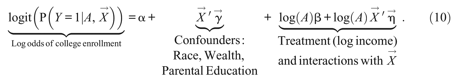
The second statistical model we consider focuses on nonlinearity: we specify a generalized additive model in which the log-odds of college enrollment are an additive (no interactions) function of parental income $A$ and confounders $\vec{X}$ . These models conceptually align with hypothesis 1, by allowing the response to family income to be a nonlinear function more complex than the log. By assuming an additive model, we gain statistical power to more precisely learn a nonlinear response surface such that the log-odds of college enrollment may follow a potentially nonlinear function of log income, represented by the smooth function $s$ .

\begin{matrix} \underset{Log odds of college enrollment}{\underset{︸}{logit (P (Y = 1 ∣ A, \vec{X}))}} = α + \underset{\begin{matrix} Confounders : \\ Race, Wealth, \\ Parental Education \end{matrix}}{\underset{︸}{{\vec{X}}^{'} \vec{γ}}} + \underset{\begin{matrix} Smooth function \\ of \log income \end{matrix}}{\underset{︸}{s (\log (A))}} \end{matrix} .

(11)

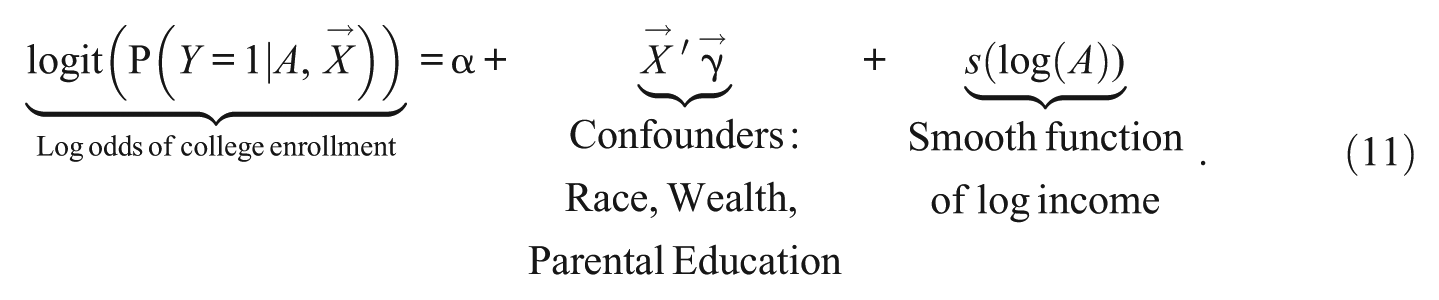
We estimate the term $s (\log (A))$ by a thin-plate spline regularized by a smoothness penalty, as operationalized in the mgcv package in R (Wood 2017). Figure 6 depicts both estimated statistical models.

The models above have distinct motivating goals: equation (10) is designed to flexibly discover effect heterogeneity while assuming a particular parametric form of nonlinearity, whereas equation (11) is designed to flexibly discover nonlinear treatment effects while assuming no interactions. Although it is theoretically possible to estimate a more complex model that incorporates both effect heterogeneity and nonlinearity, such a model would involve a large number of parameters and potentially imprecise estimation because of the available sample size. Appendix A illustrates this problem in one simple simulated setting, and Appendix B shows that a flexible machine learning estimator (a random forest) produces estimates that are high variance. We therefore focus on models that learn either additive nonlinearity or heterogeneous parameterized effects. As additional evidence to support this choice, our empirical setting is one where the treatment values (income) are strongly determined by the confounders (race, wealth, parental education). In the “General Discussion” section, we will show that in settings in which treatment assignments are strongly confounded it may be possible to model data equally well with statistical models motivated by nonlinearity or by effect heterogeneity (Figure 8). In our empirical setting, this is true: we find very similar empirical estimates by either approach (Figure C1).

A key benefit of our approach is apparent when one compares equations (10) and (11) to the simple additive regression model we describe in equation (1). The simple regression model summarizes the entire distribution of causal effects by a single coefficient $β$ under the implausible assumption that a continuous treatment is linearly and additively related to the outcome. Our preferred models instead allow the relationship to be nonlinear and heterogeneous. Our approach may appear to come at the cost of interpretability, as our models involve many more parameters. But they are actually equally interpretable once translated into estimates of the additive shift estimand: predict under the incremented treatment, predict under the factual treatment, difference, and average over units (equations 8 and 9).

Results

Our results suggest the probability of college enrollment increases substantially over the family income distribution: fewer than one in three students at the bottom decile of the income distribution enroll in college by age 21, whereas more than three in four of those at the top decile of the distribution enroll (see Figure 5). The gap in the probability of college enrollment is sizable even for small differences in family income. For each child, the predicted probability of college enrollment is 3.1 percentage points (95 percent confidence interval = 2.8 percent to 3.4 percent) higher than the predicted probability for a hypothetical child with an income $10,000 lower.

Figure 5.

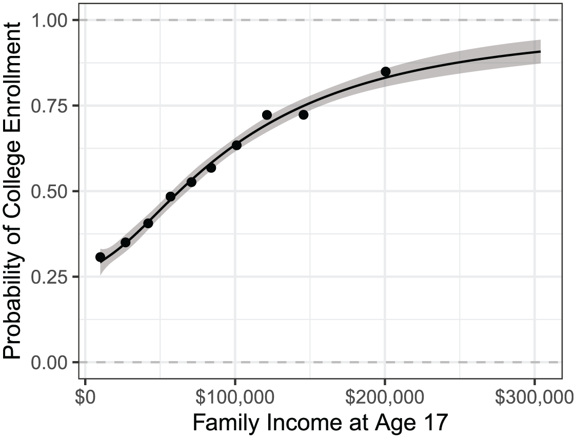
Descriptive result: family income strongly predicts college enrollment.

The results reported in Figure 5 represent a descriptive pattern. Next, we consider a causal effect estimate of the relationship between family income and children’s educational attainment. To produce a single average effect estimate, we first estimate the additive shift estimand ${\hat{τ}}_{i}$ for each child: we use the interactive logistic regression model to compare the predicted probability of college enrollment for child $i$ as observed to the predicted probability for a hypothetical child who shares the same categories of race, parental education, and family wealth of child $i$ but has an income $10,000 higher. We then average across children to produce a succinct summary statistic: the average difference in the probability of college enrollment for a $10,000 family income increment is 1.7 percentage points (95 percent confidence interval = 1.4 percent to 2.1 percent). Although our results are limited by measuring only three confounders, they are key confounders. Indeed, these three confounders account for nearly half of the association between family income and college enrollment (recall that the comparable descriptive estimate from Figure 5 was 3.1 percentage points).

We now turn to how the probability of college enrollment changes as a function of family income within population subgroups, taking a particular set of confounder values. Figure 6 shows these curves as estimated by the interactive logistic regression model and the generalized additive model. Similar to the unadjusted descriptive curve in Figure 5, the estimated curve within nearly every subpopulation shows an upward trend: the probability of college enrollment increases with family income. Results suggest nonlinear patterns across family income, supporting hypothesis 1, and effect heterogeneity by family wealth, supporting hypothesis 2. Additionally, the curves are flatter among the subgroups that correspond to children from families in which two parents completed college, indicating that college enrollment is less responsive to family income in these families, supporting hypothesis 3.

Figure 6.

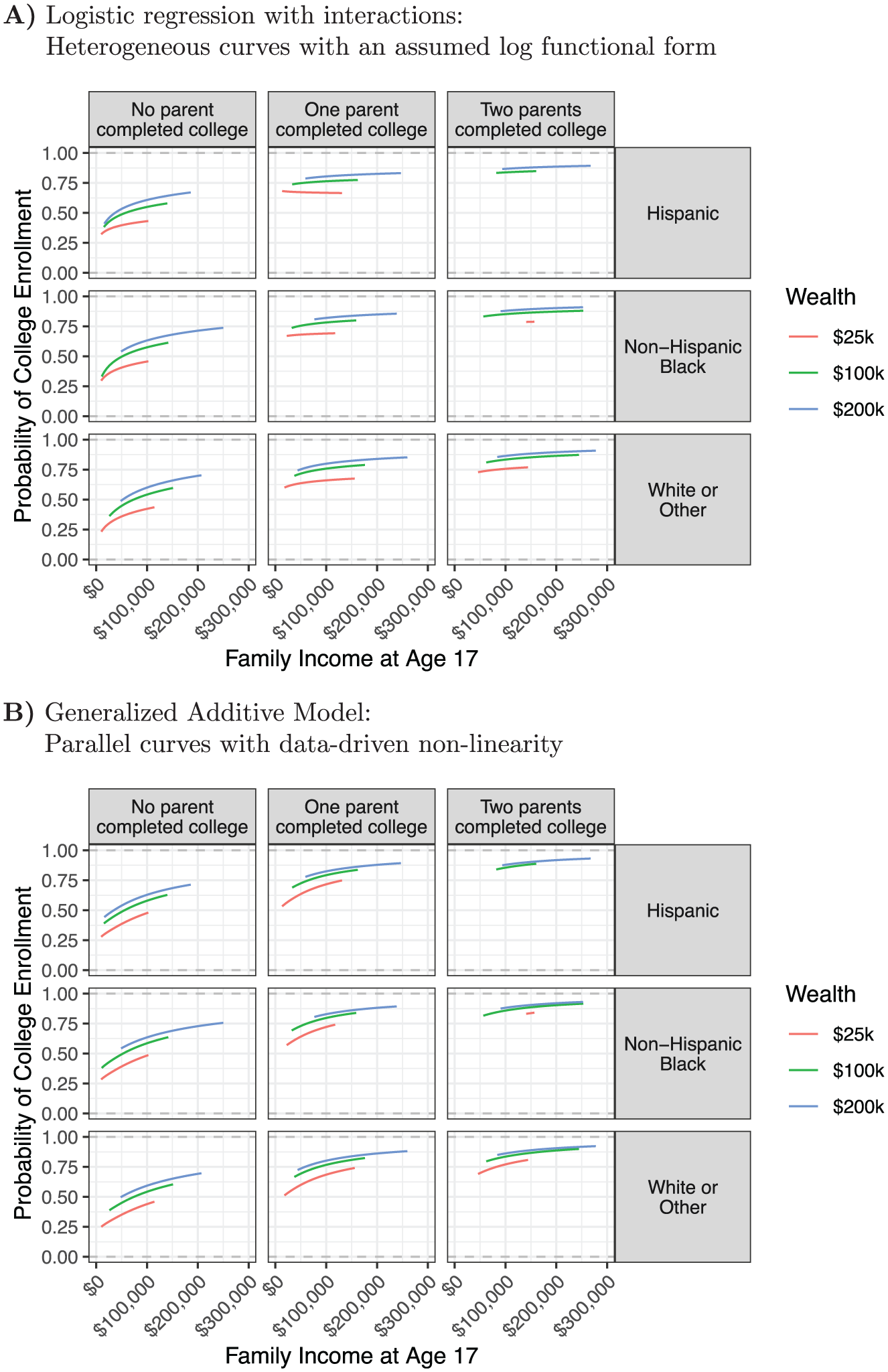
Models for causal estimation: family income effects on college enrollment are nonlinear and heterogeneous. (A) Logistic regression with interactions: Heterogeneous curves with an assumed log functional form. (B) Generalized additive model: Parallel curves with data-driven non-linearity.

Comparing across modeling approaches, Figure 6 shows remarkably similar curves estimated by either approach: interactive logistic regressions or generalized additive models. This similarity may be surprising: the first model assumes the log-odds of college enrollment are an interactive function of confounders and log family income, whereas the second model assumes the log-odds of college enrollment are an additive function of confounders and a data-driven smooth function of family income. The models seem, in theory, quite different. Nevertheless, their implications are very similar. Figure C1 further confirms this similarity by showing that the estimated value of the additive shift estimand for each unit tends to be similar under both approaches. We suspect the near equivalence of the estimates arises because of strong confounding. With strong confounding, models that focus on effect heterogeneity and models that focus on additive nonlinearity (here on the logit scale) can have very similar empirical implications (see Figure 8 in the “Discussion” section). It is also possible that the log functional form closely approximates the true pattern of nonlinearity. Alternatively, our sample size may be too small for the flexible smooth functions to learn a more complex pattern.

Using the modeled curves in Figure 6, we next produce aggregate estimates that summarize the additive shift estimand for population subgroups: how the probability of college enrollment changes, on average, for a $10,000 increase in family income over a particular set of units (see Figure 7). Because the results are very similar under both modeling approaches (columns), we discuss them together. The first row of Figure 7 reports estimates by terciles of family income. Consistent with hypothesis 1, the average causal effect in the bottom tercile of family income is more than three times larger than in the top tercile. In support of hypothesis 2, the average causal effect is approximately twice as large in the bottom tercile of family wealth compared with the top tercile. In support of hypothesis 3, income is more consequential for children’s college enrollment when parents do not hold college degrees. All three conclusions are the same under either modeling approach, with nearly identical estimates.

Figure 7.

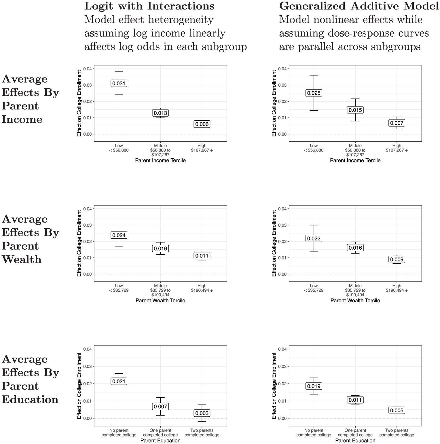
Models for heterogeneous effect estimation: family income effects differ across population subgroups.

As a second approach to summarize effect heterogeneity, Table 1 stratifies the population by the estimated conditional average treatment effect of a hypothetical additional $10,000 and summarizes the outcome, treatment, and covariates of these subpopulations. In the subgroup with the smallest effect, a $10,000 increase in family income would change the probability of college enrollment by between −3 and +1 percentage points. These are advantaged children with a median factual family income of about $138,000, median wealth of about $221,000, and 84 percent have at least one parent holding a four-year college degree. Notably, the lack of a causal effect in this advantaged subgroup cannot be interpreted as simply a ceiling effect: about 79 percent of the subgroup enrolled in college, so there is room for college enrollment to rise by up to 21 percentage points. Yet a $10,000 boost to family income raises the probability by only about 1 percentage point at most. The subgroup for whom the hypothetical income boost would be most consequential has notably large effects: a $10,000 increase in family income would increase the probability of college enrollment between +2 and +13 percentage points. These are disadvantaged children with a median family income of about $25,000, median wealth of $10,000 (the bottom code we enforced on this measure), and 97 percent of whom have no parent who holds a four-year college degree. Partitioning the sample by the estimated effect size and summarizing confounders reinforces our conclusions: a small increase in family income is most consequential for disadvantaged population subgroups.

Table 1.

Subgroup Characteristics by Estimated Effects of Family Income.

Summary Measure	Bottom Quartile of Effect Size	Middle 50% of Effect Size	Top Quartile of Effect Size
Range of effect sizes	−.03 to .01	.01 to .02	.02 to .13
Factual outcome: proportion enrolled in college	.79	.55	.35
Median income	$138,235	$81,299	$25,184
Median wealth	$221,483	$89,322	$10,000
Proportion with two parents who completed college	.36	.01	.00
Proportion with one parent who completed college	.48	.09	.03
Proportion with no parent who completed college	.16	.90	.97
Proportion Hispanic	.12	.12	.16
Proportion non-Hispanic Black	.09	.13	.26
Proportion White or other	.79	.75	.59

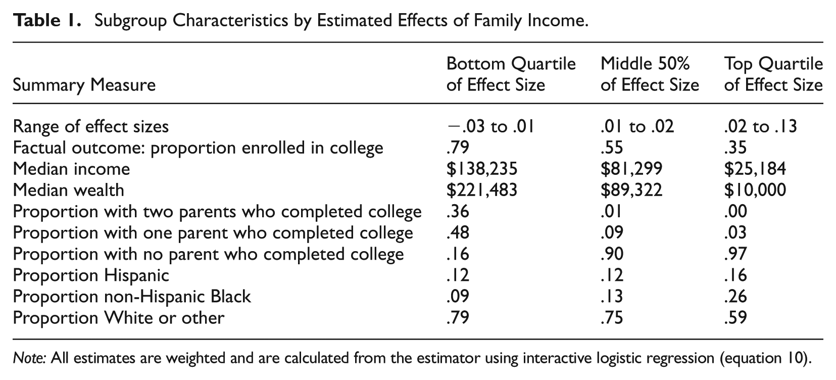
Note: All estimates are weighted and are calculated from the estimator using interactive logistic regression (equation 10).

Empirical Illustration Discussion

Our empirical illustration offers insights into an important question for social stratification research and policy: for whom does family income most strongly affect educational attainment? Researchers have extensively documented that material conditions during early childhood predict later-life outcomes (Chetty et al. 2014; Duncan, Kalil, and Ziol-Guest 2018; Duncan et al. 1998; Heckman 2006). Instead of focusing on whether income matters, we used additive shift estimands to address questions about income’s nonlinear and heterogeneous effects. We find that small differences in family income are most consequential for college enrollment among low-income families, low-wealth families, and families in which neither parent completed college.

Our empirical results raise new questions about the connection between family economic inequality and children’s educational inequality. The current period is marked by both rising income inequality (Piketty and Saez 2003) and stalled educational expansion (Voss et al. 2024). If college enrollment is especially responsive to changes in family income at upper-income values, then a rising upper tail of the income distribution could reshape who enrolls in college. But our result suggests college enrollment is especially responsive to income at lower income values. Thus, inequality in college enrollment may be more responsive to changes in economic inequality at the bottom of the distribution. Future work should explore this connection.

Heterogeneous effects of family income also point toward a new set of priorities for causal identification strategies that complement existing priorities. Past scholarship has often prioritized designs with strong internal validity. For example, Dynarski (2003, Table 2) showed that a financial transfer averaging $6,700 per year increased college enrollment by 18 percentage points by analyzing changes in a Social Security program to support the college costs of children with a deceased parent. This evidence has strong internal validity but speaks to only one subpopulation: individuals with a deceased parent who were eligible for the program. As another example, Manoli and Turner (2018) use kinks in the earned income tax credit (EITC) to show that a $1,000 transfer increases the probability of college enrollment by 1.3 percentage points among those whose family income is $12,780, but with no effect at a different kink point where family income is $40,964 (for a similar design, see Dahl and Lochner 2012). Studies such as these, which prioritize internal validity, will always hold an essential place in research on the effect of family income. But if the effect of family income is heterogeneous, their implications are bound to the subpopulations to which they speak. We took a different path by prioritizing external validity, seeking to summarize effects over the entire population. These two research strategies are complementary. Future research should use both econometric designs with strong internal validity and selection-on-observables designs, which, although weaker in terms of internal validity, can better explore the distribution of effect sizes across the population.

General Discussion

Causal questions involving continuous treatment variables are, in many ways, analogous to those involving binary treatment variables, but they invite qualitatively distinct considerations. With many potential outcomes for each unit, there are many possible causal estimands, some of which are more tractable than others. We demonstrated how additive shift estimands enable credible inferences that avoid extrapolation and support the exploration of effect variation across the population.

Effect Heterogeneity and Nonlinearity: Exploring Variation That May Be Difficult to Disentangle

We emphasized two conceptual axes of variation: effect heterogeneity and nonlinearity. Effect heterogeneity is analogous to the questions asked with binary treatments: the effect of a treatment $A$ may differ across subpopulations defined by pretreatment variables $\vec{X}$ . A continuous treatment, however, also motivates a new set of questions about nonlinearity: the effect of a small increment to treatment $A$ may depend on the initial value of that treatment. These are two distinct axes of variation in effects. Yet in our empirical example, statistical models motivated by either approach yield the same conclusions for an additive shift estimand. Here we generalize this result, showing in a stylized simulation how effect heterogeneity and nonlinearity may be difficult to disentangle in settings with strong measured confounding. Additive shift estimands are nonetheless well-defined and identified in these settings, and can be used to explore population variation without disentangling effect heterogeneity from nonlinearity.

Figure 8 considers a hypothetical sample divided into three subgroups by confounder values $X = 1$ , $X = 2$ , and $X = 3$ . Suppose each confounder subgroup has its own range of treatment values in the observed sample, so that every treatment value is observed in only one confounder subgroup. We assume for illustration that each subgroup could in theory be observed at every treatment value (positivity holds globally; $f_{A ∣ X = x} (a) > 0$ for all $a, x$ ), but the treatment density is sufficiently low that some regions are not observed in some subgroups in the sample. This is a case of strong measured confounding, analogous to how family income (a treatment) has different support across parent education (a confounder). We illustrate two data-generating processes (DGPs) that are equally consistent with these sample data: (1) each preexisting population subgroup has a linear dose-response curve with intercepts and slopes that are heterogeneous across subgroups, or (2) all preexisting population subgroups share a single dose-response curve that is not linear. More generally, the second process could involve nonlinear curves that are parallel across subgroups, differing only in their intercepts. These two DGPs coincide in the observed sample; the sample cannot adjudicate between them. The ambiguity is inconsequential for an additive shift estimand; the effect of a small increase in treatment is the same at every point regardless of which DGP is true. Yet for population-average dose-response curve estimands, the distinction matters. At every treatment value $a$ , the population-average dose-response curve from our illustrative linear heterogeneous DGP is higher than the population-average dose-response curve from our illustrative nonlinear homogeneous DGP. The data are consistent with many values of $E (Y^{a})$ . The reason for this ambiguity is that $E (Y^{a})$ is an estimand that requires extrapolation away from the observed data. The average additive shift estimand for a small increase (e.g., 0.05) takes the same value in this illustration regardless of which DGP is true.

Figure 8.

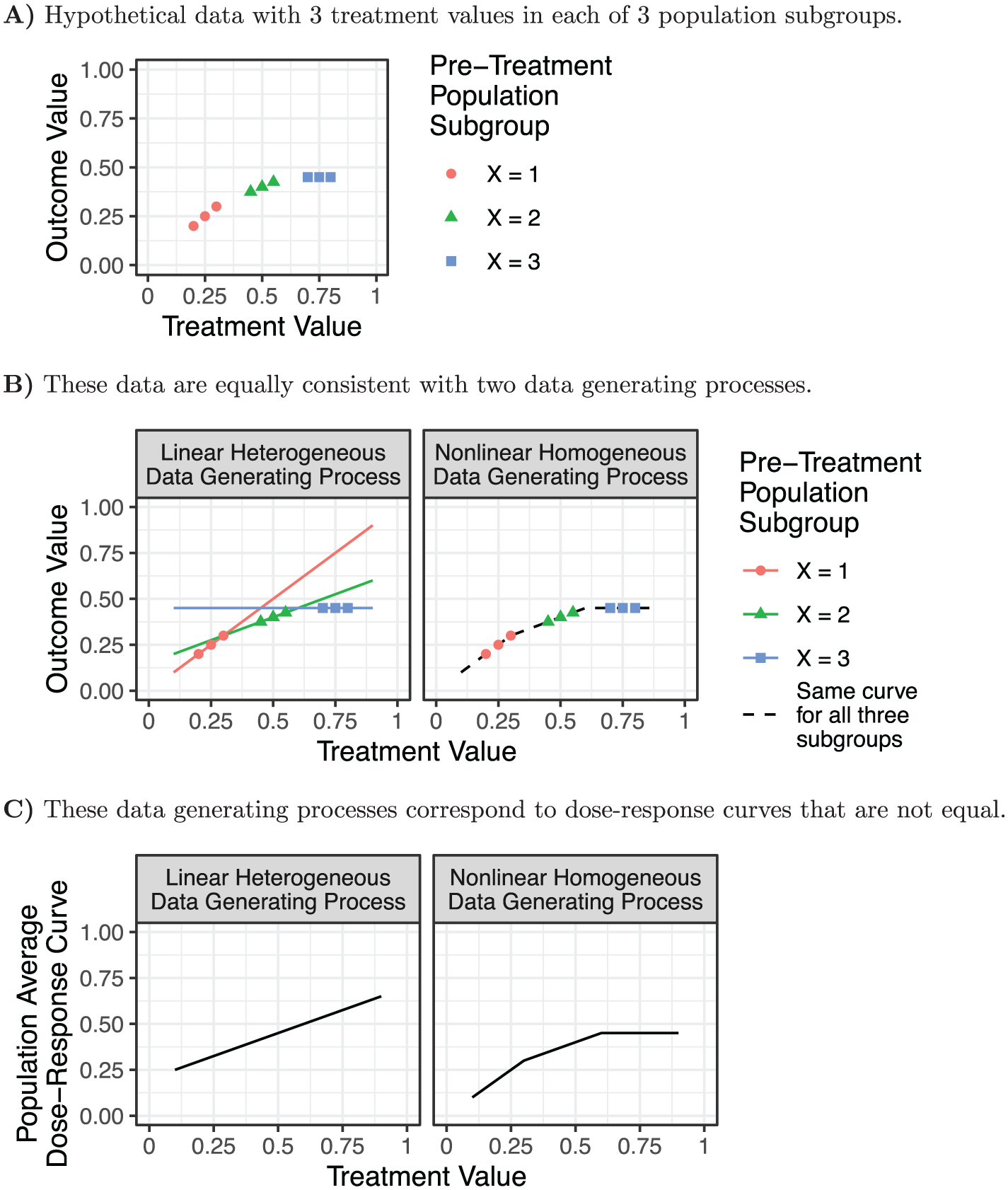
Nonlinearity and effect heterogeneity: empirical equivalence under strong confounding. (A) Hypothetical data with three treatment values in each of three population subgroups. (B) These data are equally consistent with two data-generating processes. (C) These data-generating processes correspond to dose-response curves that are not equal.

This illustration is an extreme case, but there may be many social science settings in which treatments are strongly determined by confounders. In these settings, it may be empirically challenging to adjudicate between nonlinearity and effect heterogeneity. The resulting shape of an estimated population-average dose-response curve may depend on modeling assumptions that are not easy to test empirically. Rather than engaging in these debates with limited data, researchers who adopt additive shift estimands can study an estimand that does not require a choice between models equally consistent with the observed data.

Conclusions

Social scientists routinely work with exposures that are at least theoretically continuous: income, wealth, parental work hours, minutes spent reading per day, neighborhood crime rates, and so on. For researchers interested in causal inference who might otherwise dichotomize these treatments, our approach offers an alternative strategy that allows the direct study of exposures in their continuous form. Because many of these exposures are themselves strongly shaped by other stratification processes, we suspect that many such applications will benefit from additive shift estimands that remain well defined in the presence of strong measured confounding. This framework can support future efforts to uncover not only whether numeric treatments have large effects, but also for whom and under what conditions.

Footnotes

Appendix A: Simulation: Heterogeneous Nonlinearity Can Be Difficult to Estimate

Effect heterogeneity and nonlinearity are distinct concepts that can coexist (see Figure 2). Consequently, researchers may seek an estimator that can estimate a nonlinear response curve that is also heterogeneous across population subgroups. However, estimation of patterns that are both nonlinear and heterogeneous can be statistically challenging. In small to moderate samples, one may prefer an estimator that focuses on either heterogeneity (as in equation 10) or additive nonlinearity (as in equation 11). This section presents a simulation illustrating the estimation difficulties in a specific setting.

Figure A1 illustrates a setting with five population subgroups labeled $X = 1, \dots, 5$ , in which the treatment $A$ is uniformly distributed between 0 and 1. Unlike strong confounding, the full range of treatment values is observed in each population subgroup. We consider two DGPs: an additive DGP with homogeneous effects and an interactive DGP with effect heterogeneity. In the additive DGP, outcome $Y$ responds to treatment $A$ by the same functional form in every population subgroup. In the interactive DGP, the functional form by which $A$ affects $Y$ differs across subgroups. For each DGP, we consider two estimators. The additive nonlinear model is a generalized additive model that estimates a unique intercept for each subgroup defined by $X$ and a shared smooth response function $s (A)$ capturing the change in $Y$ resulting from changes in the treatment. We estimate $s (A)$ by a thin plate spline (Wood 2017); see the section “Identification and Estimation” for details. The interactive nonlinear model estimates a separate nonlinear response surface $s_{x} (A)$ for each subgroup defined by a possible confounder value $X = x$ . We score each model by root mean squared error for additive shift estimands: the square root of the mean squared difference between the estimated additive shift estimand and the true additive shift estimand at the treatment and $X$ value of each unit. This performance metric is not possible in real data, but it is possible in simulation because the true effects are known.

The simulation shows several results. As expected, when the true DGP is additive, the additive nonlinear estimator has better performance (lower error) than the interactive nonlinear estimator. What may be more surprising is that, even in a truly interactive DGP, the additive estimator performs better at smaller sample sizes. Only at larger sample sizes ( $n > 300$ ) does the interactive estimator outperform the additive estimator in the nonlinear DGP. The sample size demands in this simulation may also understate those in more realistic applications: our simulation had only one pretreatment covariate with five values, whereas in practice, a researcher may have many pretreatment covariates with many values. The trade-off between model complexity (nonlinearity and interactions) as a function of sample size and number of predictors is an open question.

Appendix B: Simulation: Forests Can Produce High-Variance Estimates

The main text focuses on models that assume global or local smoothness, including parametric logistic regression and generalized additive models. These approaches model the response surface as a function in which the outcome $Y$ changes smoothly with changes in treatment $A$ , which may be useful when one’s goal is to predict the effect of a small change in the treatment. Here we consider an alternative estimation approach, forests, that has good predictive performance in other settings but lacks this smoothness property. We demonstrate that, in at least one simulation, forest-based estimators yield a locally bumpy response surface, resulting in high-variance additive shift estimand estimates. This is true even when we apply a local linear forest that applies a locally linear estimator on top of an estimated forest (Friedberg et al. 2020). Thus, despite the demonstrated usefulness of trees and forests for causal inference for the heterogeneous effects of binary treatments (Athey, Tibshirani, and Wager 2019; Brand et al. 2021), further advances may be needed before these approaches can serve as reliable estimators of additive shift estimands.

Figure B1 presents the simulation and results. We consider two DGPs. In both DGPs, a treatment variable $A$ follows a standard normal distribution and is unconfounded. In our first DGP, the log-odds of a binary outcome are a linear function of treatment $A$ , so that a logistic regression with $A$ as a linear predictor is correctly specified. In the second DGP, the log-odds of the outcome are a nonlinear function of $A$ , so that a logistic regression with $A$ specified as a linear function is misspecified. Under both DGPs, we consider three estimators: logistic regression, random forest estimated by the regression_forest function in the grf package, and a local linear forest estimated by the ll_regression_forest function in the same package. For both forest estimators, we let the algorithm automatically tune all hyperparameters and otherwise leave all options at their defaults.

As shown in Figure B1, the logistic regression produces a very accurate response surface estimate in the DGP where it is correctly specified and a less accurate response surface estimate in the DGP where it is incorrectly specified. The forest estimators consistently adapt to the response surface to produce a reasonably close fit, and the forests outperform logistic regression in terms of predicting conditional means in the DGP where the logistic regression is misspecified. Yet, in both DGPs, the logistic regression produces more accurate estimates of additive shift estimands. The reason is that the forest estimators produce locally bumpy response surfaces, and these local bumps result in additive shift estimands that are either highly positive or highly negative across the distribution of the treatment. Thus, although the forest estimators produce estimates of conditional means with adequately low variance and outperform logistic regression in predicting conditional means in one setting, they are inferior to logistic regression for the goal of estimating additive shift estimands in both settings.

These results are based on only one simulation, and the relative performance of forest versus logistic regression estimators is likely to vary across settings depending on the available data and the extent to which nonlinear and heterogeneous effects may be poorly captured by logistic regression. Yet this simulation serves as a cautionary note that estimators such as forests, which produce locally bumpy rather than locally smooth response surfaces, may be poor estimators of additive shift estimands.

Appendix C: Comparison of Estimators for Additive Shift Estimands

Figure C1 depicts the estimated value of the additive shift estimand for each unit under both estimation approaches considered in the main text. The figure shows that the estimates are substantively similar regardless of whether we use the interactive logistic regression or the generalized additive model specification.

Appendix D: Causal Identification Proof

Our causal identification is standard, but we provide the proof below for completeness.

(12)

τ (\vec{x}, a) = E (Y^{a + δ} - Y^{a} ∣ \vec{X} = \vec{x}, A = a) our causal estimand

(13)

\begin{matrix} = E (Y^{a + δ} ∣ \vec{X} = \vec{x}, A = a) \\ - E (Y^{a} ∣ \vec{X} = \vec{x}, A = a,) by linearity of expectation \end{matrix}

(14)

\begin{matrix} = E (Y^{a + δ} ∣ \vec{X} = \vec{x}, A = a + δ) \\ - E (Y^{a} ∣ \vec{X} = \vec{x}, A = a) by conditional exchangeability \end{matrix}

(15)

\begin{matrix} = E (Y ∣ \vec{X} = \vec{x}, A = a + δ) \\ - E (Y ∣ \vec{X} = \vec{x}, A = a) by consistency \end{matrix}

In the proof, (12) is our causal estimand, (13) is by linearity of expectation, (14) is by conditional exchangeability, and (15) is by consistency. The final line is our empirical estimand, which we estimate by predicting the two quantities using our outcome model.

Acknowledgements

We thank the Inequality Data Science Lab at the University of California, Los Angeles, and Florencia Torche for helpful discussions and feedback relevant to this project, as well as seminar participants at the New York University Department of Sociology, University of Pennsylvania Department of Sociology, University of Washington Center for Statistics in the Social Sciences, Linköping University Institute for Analytical Sociology, and the annual meetings of the American Sociological Association and the Population Association of America.

Authors’ Note

We did not use artificial intelligence tools to facilitate writing this article; we did use artificial intelligence tools to check our human-written replication package for coding errors.

ORCID iDs

Ian Lundberg

Jennie E. Brand

Funding

The authors disclosed receipt of the following financial support for the research, authorship, and/or publication of this article: Research reported in this article was supported by the National Science Foundation under award 2104607 and by the Eunice Kennedy Shriver National Institute of Child Health and Human Development of the National Institutes of Health under award P2CHD041022.

Declaration of Conflicting Interests

The authors declared no potential conflicts of interest with respect to the research, authorship, and/or publication of this article.

Data Note

Replication code is available at Dataverse ().

Notes

Author Biographies

Ian Lundberg is an assistant professor of sociology at the University of California, Los Angeles, and an affiliate of the California Center for Population Research and the Center for Social Statistics.

Jennie E. Brand is a professor of sociology and a professor of statistics and data science at the University of California, Los Angeles. She is codirector of the Center for Social Statistics and an affiliate of the California Center for Population Research. She is the author of Overcoming the Odds: The Benefits of Completing College for Unlikely Graduates (Russell Sage, 2023).

References

Acemoglu

Daron

Pischke

Jörn-Steffen

. 2001. “Changes in the Wage Structure, Family Income, and Children’s Education.” European Economic Review 45(4–6):890–904.

Athey

Susan

Tibshirani

Julie

Wager

Stefan

. 2019. “Generalized Random Forests.” Annals of Statistics 47(2):1148–78.

Bailey

Martha J.

Dynarski

Susan M.

2011. “Gains and Gaps: Changing Inequality in U.S. College Entry and Completion.” NBER Working Paper No. 17633. Cambridge, MA: National Bureau of Economic Research.

Belley

Philippe

Lochner

Lance

. 2007. “The Changing Role of Family Income and Ability in Determining Educational Achievement.” Journal of Human Capital 1(1):37–89.

Bloome

Deirdre

Dyer

Shauna

Zhou

Xiang

. 2018. “Educational Inequality, Educational Expansion, and Intergenerational Income Persistence in the United States.” American Sociological Review 83(6):1215–53.

Brand

Jennie E

. 2023. Overcoming the Odds: The Benefits of Completing College for Unlikely Graduates. New York: Russell Sage.

Brand

Jennie E.

Xie

. 2010. “Who Benefits Most from College? Evidence for Negative Selection in Heterogeneous Economic Returns to Higher Education.” American Sociological Review 75(2):273–302.

Brand

Jennie E.

Jiahui

Koch

Bernard

Geraldo

Pablo

. 2021. “Uncovering Sociological Effect Heterogeneity Using Tree-Based Machine Learning.” Sociological Methodology 51(2):189–223.

Brand

Jennie E.

Zhou

Xiang

Xie

. 2023. “Recent Developments in Causal Inference and Machine Learning.” Annual Review of Sociology 49:81–110.

10.

Chen

Xianglei

Lauff

Erich

Arbeit

Caren A.

Henke

Robin

Skomsvold

Paul

Hufford

Justine

. 2017. “Early Millennials: The Sophomore Class of 2002 a Decade Later.” NCES 2017-437. Washington, DCT: National Center for Education Statistics.

11.

Cheng

Siwei

Brand

Jennie E.

Zhou

Xiang

Xie

Hout

Michael

. 2021. “Heterogeneous Returns to College over the Life Course.” Science Advances 7(51):eabg7641.

12.

Chetty

Raj

Hendren

Nathaniel

Kline

Patrick

Saez

Emmanuel

Turner

Nicholas

. 2014. “Is the United States Still a Land of Opportunity? Recent Trends in Intergenerational Mobility.” American Economic Review 104(5):141–47.

13.

Dahl

Gordon B.

Lochner

Lance

. 2012. “The Impact of Family Income on Child Achievement: Evidence from the Earned Income Tax Credit.” American Economic Review 102(5):1927–56.

14.

Díaz

Iván

van der Laan

Mark J.

2013. “Targeted Data Adaptive Estimation of the Causal Dose–Response Curve.”Journal of Causal Inference 1(2):171–92.

15.

Díaz

Iván

van der Laan

Mark J.

2018. “Stochastic Treatment Regimes.” pp. 219–32 in Targeted Learning in Data Science: Causal Inference for Complex Longitudinal Studies, edited by Van der Laan

M. J.

Rose

New York: Springer.

16.

Díaz Muñoz

Iván

van der Laan

Mark J.

2012. “Population Intervention Causal Effects Based on Stochastic Interventions.”Biometrics 68(2):541–49.

17.

Duncan

Greg J.

Kalil

Ariel

Ziol-Guest

Kathleen M.

2018. “Parental Income and Children’s Life Course: Lessons from the Panel Study of Income Dynamics.” Annals of the American Academy of Political and Social Science 680(1):82–96.

18.

Duncan

Greg J.

Murnane

Richard J.

, eds. 2011. Whither Opportunity? Rising Inequality, Schools, and Children’s Life Chances. New York: Russell Sage.

19.

Duncan

Greg J.

Yeung

W. Jean

Brooks-Gunn

Jeanne

Smith

Judith R.

1998. “How Much Does Childhood Poverty Affect the Life Chances of Children?” American Sociological Review 63(3):406–23.

20.

Dynarski

Susan M

. 2003. “Does Aid Matter? Measuring the Effect of Student Aid on College Attendance and Completion.” American Economic Review 93(1):279–88.

21.

Elwert

Felix

Pfeffer

Fabian T.

2022. “The Future Strikes Back: Using Future Treatments to Detect and Reduce Hidden Bias.” Sociological Methods & Research 51(3):1014–51.

22.

Farkas

George

. 2018. “Family, Schooling, and Cultural Capital.” Pp. 3–38 in Handbook of the Sociology of Education in the 21st Century, edited by Schneider

New York: Springer.

23.

Friedberg

Rina

Tibshirani

Julie

Athey

Susan

Wager

Stefan

. 2020. “Local Linear Forests.” Journal of Computational and Graphical Statistics 30(2):503–17.

24.

Gill

Richard D.

Robins

James M.

2001. “Causal Inference for Complex Longitudinal Data: The Continuous Case.” Annals of Statistics 29(6):1785–1811.

25.

Goldrick-Rab

Sara

Kelchen

Robert

Harris

Douglas N.

Benson

James

. 2016. “Reducing Income Inequality in Educational Attainment: Experimental Evidence on the Impact of Financial Aid on College Completion.” American Journal of Sociology 121(6):1762–1817.

26.

Haneuse

Sebastien

Rotnitzky

Andrea

. 2013. “Estimation of the Effect of Interventions That Modify the Received Treatment.” Statistics in Medicine 32(30):5260–77.

27.

Hanmer

Michael J.

Kalkan

Kerem Ozan

. 2013. “Behind the Curve: Clarifying the Best Approach to Calculating Predicted Probabilities and Marginal Effects from Limited Dependent Variable Models.” American Journal of Political Science 57(1):263–77.

28.

Heckman

James J

. 2006. “Skill Formation and the Economics of Investing in Disadvantaged Children.” Science 312(5782):1900–1902.

29.

Hernán

Miguel A.

Robins

James M.

2021. Causal Inference: What If. Boca Raton, FL: Chapman & Hall/CRC.

30.

Hirano

Keisuke

Imbens

Guido W.

2004. “The Propensity Score with Continuous Treatments.” Pp. 73–84 in Applied Bayesian Modeling and Causal Inference from Incomplete-Data Perspectives, edited by Gelman

Meng

X.-L.

Chichester, UK: Wiley Ltd.

31.

Holland

Paul W

. 1986. “Statistics and Causal Inference.” Journal of the American Statistical Association 81(396):945–60.

32.

Houle

Jason N

. 2014. “Disparities in Debt: Parents’ Socioeconomic Resources and Young Adult Student Loan Debt.” Sociology of Education 87(1):53–69.

33.

Hout

Michael

. 1988. “More Universalism, Less Structural Mobility: The American Occupational Structure in the 1980s.” American Journal of Sociology 93(6):1358–1400.

34.

Hout

Michael

. 2012. “Social and Economic Returns to College Education in the United States.” Annual Review of Sociology 38:379–400.

35.

Hout

Michael

Janus

Alexander

. 2011. “Educational Mobility in America: 1930s–2000s.” Pp. 165–85 in Whither Opportunity? Rising Inequality, Schools, and Children’s Life Chances, edited by Duncan

G. J.

Murnane

R. J.

New York: Russell Sage.

36.

Imai

Kosuke

Van Dyk

David A.

2004. “Causal Inference with General Treatment Regimes: Generalizing the Propensity Score.” Journal of the American Statistical Association 99(467):854–66.

37.

Imbens

Guido W.

Rubin

Donald B.

2015. Causal Inference in Statistics, Social, and Biomedical Sciences. Cambridge, UK: Cambridge University Press.

38.

Jack

Anthony Abraham

. 2019. The Privileged Poor: How Elite Colleges Are Failing Disadvantaged Students. Cambridge, MA: Harvard University Press.

39.

Kennedy

Edward H.

Zongming

McHugh

Matthew D.

Small

Dylan S.

2017. “Non-parametric Methods for Doubly Robust Estimation of Continuous Treatment Effects.” Journal of the Royal Statistical Society Series B: Statistical Methodology 79(4):1229–45.

40.

King

Gary

Tomz

Michael

Wittenberg

Jason

. 2000. “Making the Most of Statistical Analyses: Improving Interpretation and Presentation.” American Journal of Political Science 44(2):341–55.

41.

Kornrich

Sabino

. 2016. “Inequalities in Parental Spending on Young Children: 1972 to 2010.” AERA Open 2(2):1–12.

42.

Kornrich

Sabino

Furstenberg

Frank

. 2013. “Investing in Children: Changes in Parental Spending on Children, 1972–2007.” Demography 50(1):1–23.

43.

Lareau

Annette

. 2003. Unequal Childhoods: Class, Race, and Family Life. Berkeley: University of California Press.

44.

Long

J. Scott

. 1997. Regression Models for Categorical and Limited Dependent Variables. Thousand Oaks, CA: Sage.

45.

Long

J. Scott

Mustillo

Sarah A.

2021. “Using Predictions and Marginal Effects to Compare Groups in Regression Models for Binary Outcomes.” Sociological Methods & Research 50(3):1284–1320.

46.

Manoli

Day

Turner

Nicholas

. 2018. “Cash-on-Hand and College Enrollment: Evidence from Population Tax Data and the Earned Income Tax Credit.” American Economic Journal: Economic Policy 10(2):242–71.

47.

Mayer

Susan E

. 1997. What Money Can’t Buy: Family Income and Children’s Life Chances. Cambridge, MA: Harvard University Press.

48.

Mize

Trenton D

. 2019. “Best Practices for Estimating, Interpreting, and Presenting Nonlinear Interaction Effects.” Sociological Science 6:81–117.

49.

Mize

Trenton D.

Doan

Long

J. Scott

. 2019. “A General Framework for Comparing Predictions and Marginal Effects across Models.” Sociological Methodology 49(1):152–89.

50.

Moore

Kelly L.

Neugebauer

Romain

van der Laan

Mark J.

Tager

Ira B.

2012. “Causal Inference in Epidemiological Studies with Strong Confounding.”Statistics in Medicine 31(13):1380–1404.

51.

Pearl

Judea

. 2009. Causality. Cambridge, UK: Cambridge University Press.

52.

Piketty

Thomas

Saez

Emmanuel

. 2003. “Income Inequality in the United States, 1913–1998.” Quarterly Journal of Economics 118(1):1–41.

53.

Powell

James L.

Stock

James H.

Stoker

Thomas M.

1989. “Semiparametric Estimation of Index Coefficients.” Econometrica 57(6):1403–30.

54.

Reardon

Sean F

. 2011. “The Widening Academic Achievement Gap between the Rich and the Poor: New Evidence and Possible Explanations.” Pp. 91–116 in Whither Opportunity? Rising Inequality, Schools, and Children’s Life Chances, edited by Duncan

G. J.

Murnane

R. J.

New York: Russell Sage.

55.

Regan

Erica P

. 2020. “Food Insecurity among College Students.” Sociology Compass 14(6):e12790.

56.

Robins

James M

. 1987. “Addendum to ‘A New Approach to Causal Inference in Mortality Studies with a Sustained Exposure Period—Application to Control of the Healthy Worker Survivor Effect.’” Computers & Mathematics with Applications 14(9–12):923–45.

57.

Rosenbaum

Paul R

. 2010. Design of Observational Studies. New York: Springer.

58.

Rothenhäusler

Dominik

Bin

. 2019. “Incremental Causal Effects.” arXiv. Retrieved June 4, 2026. https://arxiv.org/abs/1907.13258.

59.

Schneider

Daniel

Hastings

Orestes P.

LaBriola

Joe

. 2018. “Income Inequality and Class Divides in Parental Investments.” American Sociological Review 83(3):475–507.

60.

Smith

Jeffrey

. 2022. “Treatment Effect Heterogeneity.” Evaluation Review 46(5):652–77.

61.

Stuart

Elizabeth A

. 2010. “Matching Methods for Causal Inference: A Review and a Look Forward.” Statistical Science 25(1):1.

62.

Takatsu

Kenta

Westling

Ted

. 2025. “Debiased Inference for a Covariate-Adjusted Regression Function.” Journal of the Royal Statistical Society Series B: Statistical Methodology 87(1):33–55.

63.

Torche

Florencia

. 2011. “Is a College Degree Still the Great Equalizer? Intergenerational Mobility across Levels of Schooling in the United States.” American Journal of Sociology 117(3):763–807.

64.

Van der Laan

Mark J.

Petersen

Maya L.

2007. “Causal Effect Models for Realistic Individualized Treatment and Intention to Treat Rules.”International Journal of Biostatistics 3(1):Article 3.

65.

VanderWeele

Tyler J.

Hernán

Miguel A.

2013. “Causal Inference under Multiple Versions of Treatment.” Journal of Causal Inference 1(1):1–20.

66.

Voss

Kim

Hout

Michael

George

Kristin

. 2024. “Persistent Inequalities in College Completion, 1980–2010.” Social Problems 71(2):480–508.

67.

Witteveen

Dirk

Attewell

Paul

. 2020. “Reconsidering the ‘Meritocratic Power of a College Degree.’” Research in Social Stratification and Mobility 66:100479.

68.

Wood

Simon N

. 2017. Generalized Additive Models: An Introduction with R. Boca Raton, FL: CRC Press.

69.

Wooldridge

Jeffrey M

. 2005. “Unobserved Heterogeneity and Estimation of Average Partial Effects.” Pp. 27–55 in Identification and Inference for Econometric Models: Essays in Honor of Thomas Rothenberg, edited by Andrews

D.W.K.

Stock

J. H.

Cambridge, UK: Cambridge University Press.

70.

Xie

. 2013. “Population Heterogeneity and Causal Inference.” Proceedings of the National Academy of Sciences 110(16):6262–68.

71.

Young

Jessica G.

Hernán

Miguel A.

Robins

James M.

2014. “Identification, Estimation and Approximation of Risk under Interventions That Depend on the Natural Value of Treatment Using Observational Data.” Epidemiologic Methods 3(1):1–19.

72.

Zhou

Xiang

. 2019. “Equalization or Selection? Reassessing the ‘Meritocratic Power’ of a College Degree in Intergenerational Income Mobility.” American Sociological Review 84(3):459–85.

73.

Zhou

Xiang

. 2024. “Attendance, Completion, and Heterogeneous Returns to College: A Causal Mediation Approach.” Sociological Methods & Research 53(3):1136–66.

Causal Inference with a Continuous Treatment: Addressing Positivity Constraints,Nonlinearity,and Effect Heterogeneity

Abstract

Keywords

Causal Effects of a Continuous Treatment

Effect Heterogeneity and Nonlinearity: Why β Is an Inadequate Causal Estimand

The Extrapolation Problem

Credible Counterfactuals: Additive Shift Estimands

Identification and Estimation for Additive Shift Estimands

Connections to Literature in Statistics

Summary: Why Use Additive Shift Estimands

Empirical Example: Effect of Parental Income on College Enrollment

Data

Hypotheses

Identification and Estimation

Results

Empirical Illustration Discussion

General Discussion

Effect Heterogeneity and Nonlinearity: Exploring Variation That May Be Difficult to Disentangle

Conclusions

Footnotes

Appendix A: Simulation: Heterogeneous Nonlinearity Can Be Difficult to Estimate

Appendix B: Simulation: Forests Can Produce High-Variance Estimates

Appendix C: Comparison of Estimators for Additive Shift Estimands

Appendix D: Causal Identification Proof

Acknowledgements

Authors’ Note

ORCID iDs

Funding

Declaration of Conflicting Interests

Data Note

Notes

Author Biographies

References

Effect Heterogeneity and Nonlinearity: Why $β$ Is an Inadequate Causal Estimand