Application of parabolic blending for the estimation of thickness distribution in thermoformed products

Abstract

The Parabolic Blending (PB) technique has been widely used in various research fields, such as rotor noise prediction, over the last few decades. However, in the literature, PB is not utilised for the thickness prediction of thermoformed products. In this study, Polystyrene (PS) sheets of various thicknesses were thermoformed using a lab-scale thermoforming machine. Firstly, thickness distributions in thermoformed PS products were obtained by the experimental method. Then, PB was used to estimate the thickness distribution of conical semi-finished thermoformed parts. The obtained results were then compared with the ones obtained experimentally. A comparison reveals that the use of PB provides more accurate thickness values than the experimental results. As a result, PB can be utilised for the prediction of thickness distribution in thermoformed products which have been formed by the same mould.

Keywords

Thickness distribution parabolic blending thermoforming polystyrene

Introduction

Thermoforming is one of the most important processes in the plastic packaging industry. Besides, there are many types of thermoforming, such as plug assist thermoforming, vacuum forming, and pre-blow positive or negative forming according to the type of applied pressure (vacuum or positive air) and application of pre-stretching. Thermoforming is commonly used in the production of packaging for food, blisters, and almost any kind of consumer goods. Thermoforming is used not only in packaging, but also in many other areas ranging from the automobile industry to the production of toys.^1–4

Thermoforming can be described as the process of heating a flat plastic sheet or film to the proper temperature, which depends on the type of plastic. After heating, plastic is stretched into a female (negative) or male (positive) mould with the help of a vacuum of positive air pressure. The formed plastic is held in the mould while it cools and solidifies. Then, it is released from the mould. If necessary, trimming is applied as the last step.

Thermoforming provides an advantage to the manufacturer with its flexible product design and low mould cost compared to competitive production methods such as plastic injection moulding and blow moulding. Additionally, it is possible to manufacture cost effective moulds easily for prototype tooling in thermoforming. The forming of large parts can be achieved economically via thermoforming. Furthermore, the thermoforming process is almost always automated. Nevertheless, faster cycle times can be achieved than are possible through other thermoplastic forming processes. Recently, Polylactic acid (PLA) and Green Polyethylene (PE), which are biopolymers, have been used in thermoforming too. However, these materials are rarely used in packaging applications due to their high costs.

Thermoformed part quality depends on many parameters, such as thickness distribution of a product, type of thermoplastic, type of forming, forming temperature, applied vacuum or positive air pressure, visual requirements, gas permeability, and whether coating is necessary. On the other hand, thickness distribution is quite difficult to control, and it affects the rigidity and visuality of a product. If the packaged product is a food, it has an impact on the shelf life of the product.

In order to provide uniform thickness distribution, plug assist and pre-blow thermoforming are utilised. In this process, determination of the thickness distribution is achieved experimentally, hence it is a destructive method. A thermoformed product is cut into pieces, and thickness is measured at various points in the thermoformed product. Preparing the thermoformed sample for measuring and taking measurements often takes a long time. For this reason, Digital Image Correlation and Image Processing are the alternative methods which can be used for thickness measurements in thermoformed products non-destructively.

A considerable volume of literature has been published on the thickness distributions of thermoformed products. On the other hand, fewer studies can be found on using PB in the prediction of thickness distribution in thermoformed products. Most of the studies have had a focus on changing the process parameters and type of forming for uniform thickness distribution in products.^5–11 Additionally, effort has been made to study the effect of the rheological properties of thermoplastic materials on total product quality.^12,13 In recent years, a number of studies have sought to determine the desired properties of materials non-destructively. Digital Image Correlation and Image Processing are two of these methods. Gunel and Basaran¹⁴ monitored thermoformed specimens with a Panasonic GPKR222 CCD camera before testing and after thermoforming. They used Adobe® Photoshop® software to convert images from RGB mode to grey mode. They digitised the processed images using MatLAB® Image Processing Toolbox^TM software to obtain image histograms in grey scale. Finally, they managed to define stress whitening in thermoformed samples numerically. Molnar et al.¹⁵ used an image processing tool to analyse shear deformation in dry preforms and thermoformed laminates. They took and prepared photos of thermoformed laminates in order to measure the angle between warp and weft threads. The image processing technique was also used to measure the surface strains on all-PP pipes under hydrostatic pressure,¹⁶ and to measure the plastic deformation resulting from low velocity impact events.¹⁷ Gunel and Basaran¹⁸ developed a method which characterises levels of stress whitening. They used image processing to show the correlation between forming temperature and stress whitening after thermoforming.

Besides, PB is an important field of study in computer graphics. It can be used to predict all graphically expressive structures, such as rotor noise prediction,¹⁹ especially when a path needs to be followed.²⁰ For this, it is necessary to define it in such a way as to form a linear structure in the coordinate axis.

In this study, PS (SABIC® PS 825E) sheets with thicknesses of 0.9, 1, 1.25, 1.3 and 3 mm were thermoformed. For each thickness value, three samples were thermoformed using a conical mould. The thickness distributions were measured via the experimental method. The thickness distributions for the thermoformed samples were compared to each other using a graphical method. Since all of the thermoformed samples were formed using a conical mould, PB was used for the prediction of thickness distribution in the thermoformed samples with an initial thickness of 1.25 and 3 mm. PB was used for the first time in the literature for thickness prediction in thermoformed samples. Additionally, PB enabled the non-destructive determination of the thickness distributions of thermoformed products. If a package is produced by mass production, that is, if all packages are thermoformed using the same mould, prediction using PB can be an effective way to determine the thickness distribution in a thermoformed product, with an acceptable margin of error.

Experimental study

In this study, SABIC® PS 825E PS sheets were cut and prepared as squares with dimensions of 150 × 150 mm, since the thermoforming mould used in this work has a projection area of 150 × 150 mm². PS sheets with thicknesses of 0.9, 1, 1.25, 1.3 and 3 mm were thermoformed, since these sheet thicknesses are easily available in this region. In addition, most of the PS sheets which are used in cut sheet thermoforming have a thickness of between 1 and 3 mm. A conical aluminium mould, which was manufactured by machining, was used in the thermoforming of the PS sheets. Three samples were thermoformed for each thickness case. Selected physical properties of PS are provided in Table 1. The thermoforming operations were performed by a thermoforming machine (Oysan Machinery, Turkey). This thermoforming machine has a heating area of 20 × 20 cm². Since PS is an amorphous thermoplastic, it has a wide forming temperature range. Nevertheless, the forming temperature was determined using a thermal imaging camera (Testo) accurately. The average forming temperatures for the PS sheets with a thickness of 1.25 and 3 mm can be seen in Figure 1. Besides, the thermoforming process parameters are shown in Table 2.

Table 1.

Selected physical properties of PS (SABIC® PS 825E).

Properties	Units SI	Values	Test methods
Polymer properties
Melt flow rate MFR			ASTM D 1238
at 200°C and 5 kg	G × 10⁻¹ min	3
Density	Kg × m⁻³	1040	ASTM D 792
Bulk density			ASTM D 1895
Method B	Kg × m⁻³	600
Mechanical properties (Based on injection moulded test specimens)
Tensile test (Speed of testing: 5 mm × min⁻¹)			ASTM D 638
Tensile strength	MPa	24
Tensile elongation	%	45
Tensile modulus	MPa	2206
Flexural test			ASTM D 790
Flexural modulus	MPa	2108
Flexural strength	MPa	49
Izod impact notched at 23°C (Thickness of test specimens: 3 mm)	J × m⁻¹	170	ASTM D 256
Thermal properties (Based on injection moulded test specimens)
Heat deflection temperature			ASTM D 648
Method B, 455 KPa, annealed	°C	97
Vicat softening temperature			ASTM D 1525
Rate A, 1 kg × 50⁻¹°C	°C	100

Figure 1.

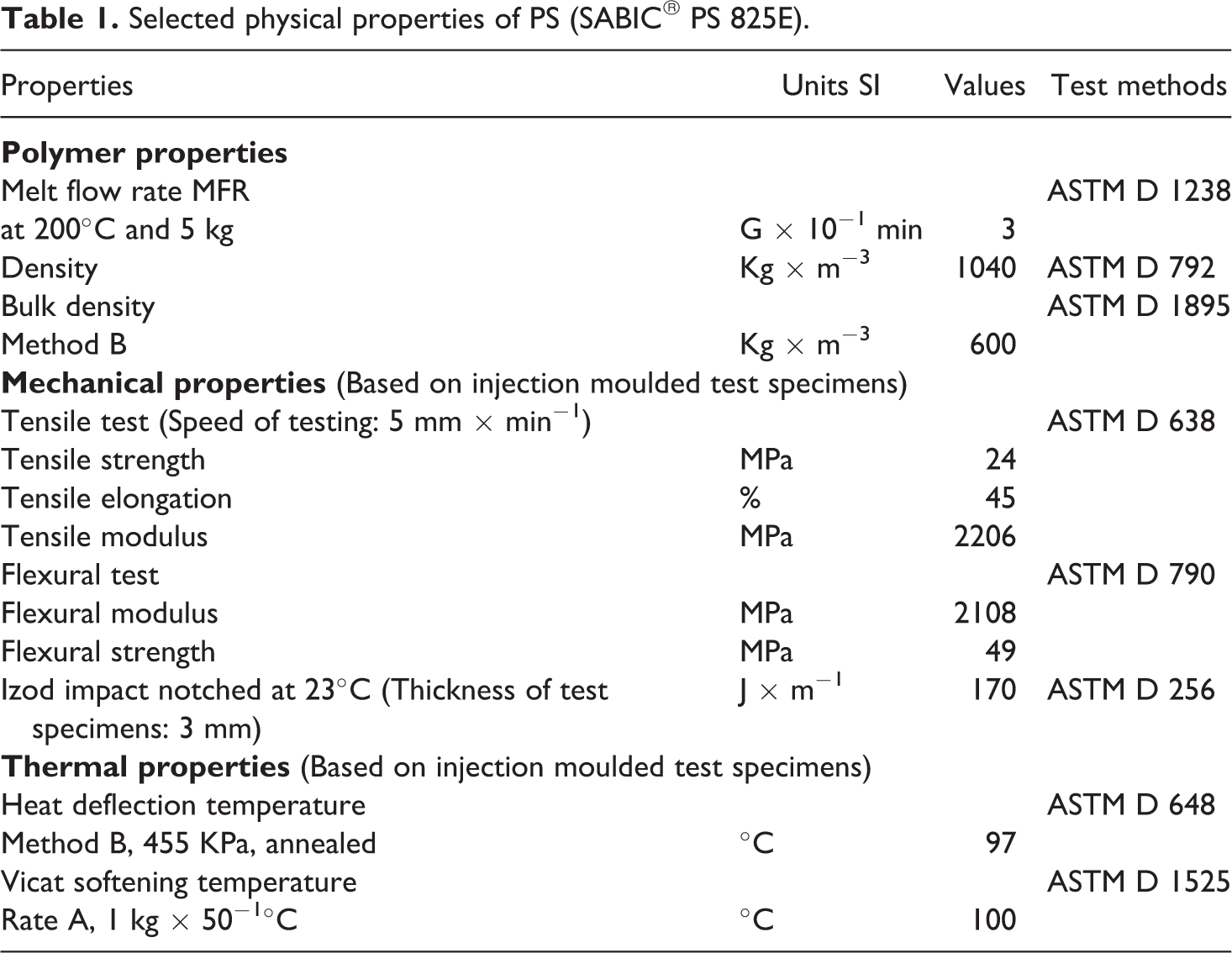
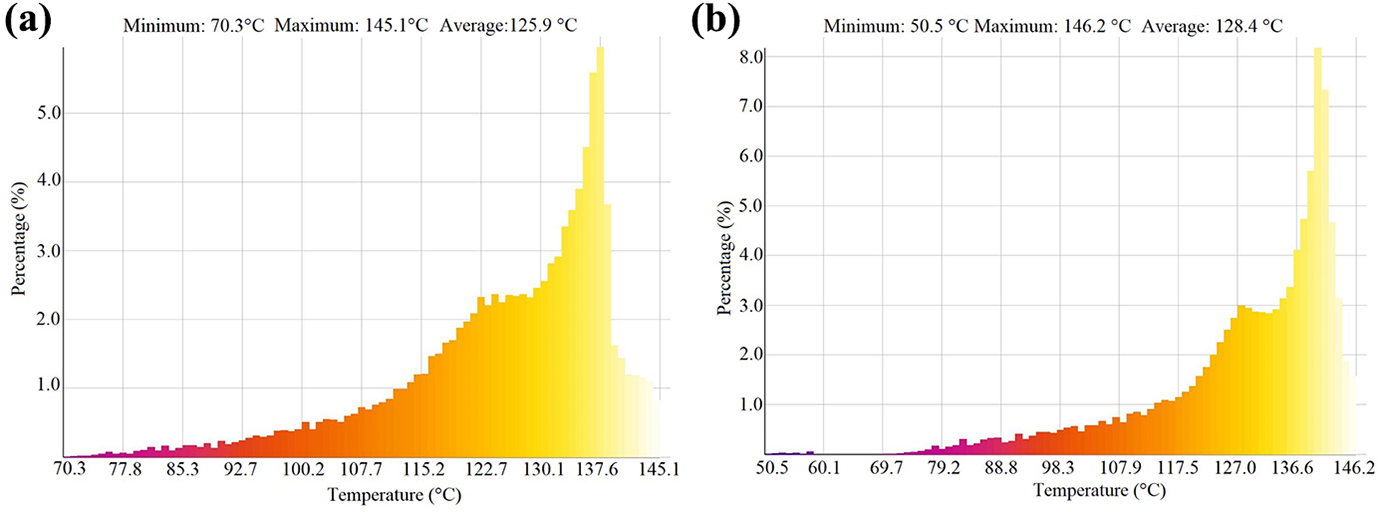
Average thermoforming temperature for PS sheets that have initial thickness values of a) 1.25 mm and b) 3 mm.

Table 2.

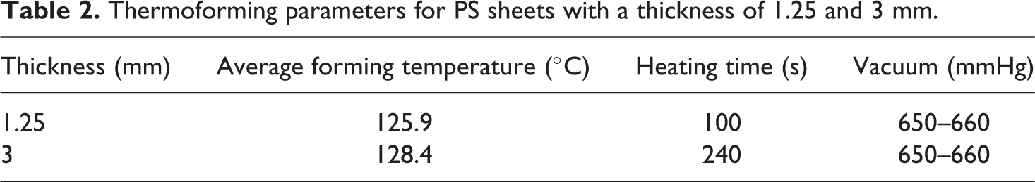
Thermoforming parameters for PS sheets with a thickness of 1.25 and 3 mm.

Thickness (mm)	Average forming temperature (°C)	Heating time (s)	Vacuum (mmHg)
1.25	125.9	100	650–660
3	128.4	240	650–660

When PS sheets with thicknesses of 0.9, 1, 1.25, 1.3 and 3 mm were thermoformed, thickness measurements were made using a digital caliper at 28 points. Selected points are given in Figure 2. Measurements were taken from the points with equal distances along a preselected path, from the centre of the base of the thermoformed sample (Point 1) to the outer edge (Point 28). However, when the thickness distribution of a conical thermoformed sample is taken into account, it should be determined where the thickness varies considerably. The thickness values changed significantly between Points 8 and 23, which are located along the base corner, the side wall, and the top corner of the sample. Because of this, from Point 8 to Point 23, only 16 points were selected for PB application. Additionally, PB was applied for only two thickness cases (1.25 and 3 mm).

Figure 2.

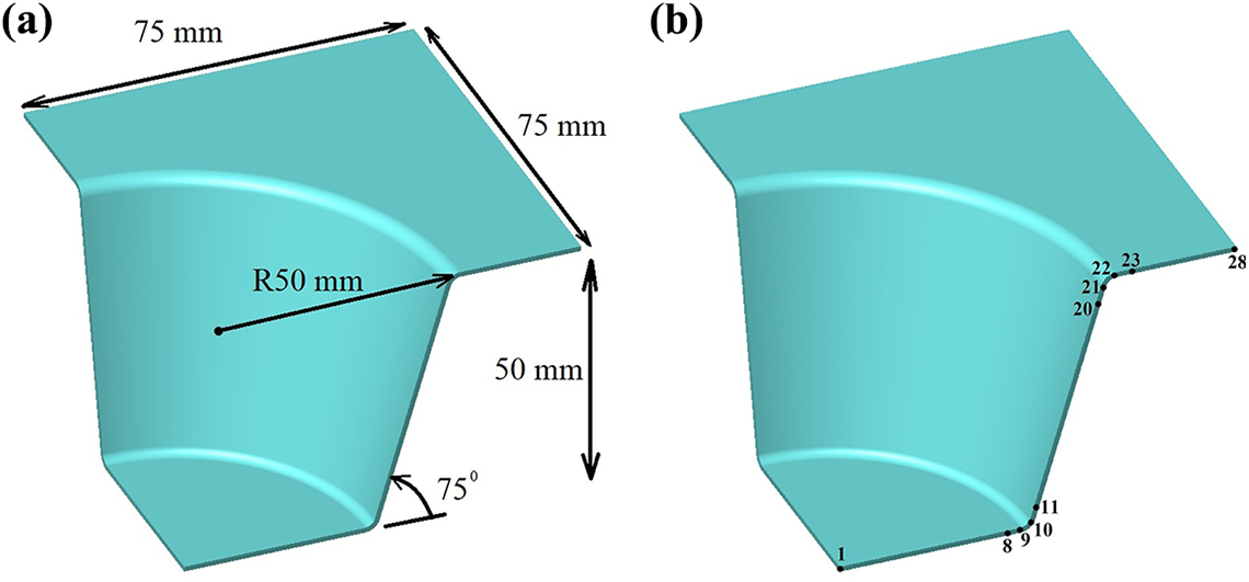
a) Dimensions and b) measuring points in a quarter of the thermoformed sample.

The variation of thicknesses with measuring points is shown in Figure 3. A considerable amount of change in thickness can be seen from Points 8 to 23. As shown in Figure 3, the thickness is nearly the same from Points 24 to 28. Therefore, only 16 measuring points were selected for the application of PB. One of the goals in this study is providing an estimation of thickness distribution for thermoformed PS samples in different initial thicknesses. For the effective application of PB and software design in the estimation process, only two thickness cases (1.25 and 3 mm) were taken into consideration.

Figure 3.

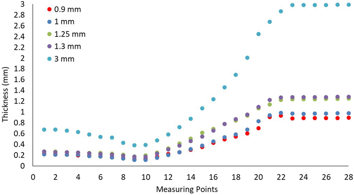
Thickness distributions for PS sheets with initial thicknesses of 0.9, 1, 1.25, 1.3 and 3 mm.

Numerical study

Initially, the obtained thickness values were transferred to the coordinate axis (x, y) for the selected thicknesses (1.25 and 3 mm). It was observed that the shape of the PS sheet measured values applied in the conical form mould was in the form of a cubic curve in the xy plane.

Since it is thought that this shape can be created with the PB method, software interface has been developed using Visual C ++ >> OpenGL in order to determine whether there is a pattern between the curve formed by the PS sheet thickness in the coordinate axis, and the curve created by the PB method.

In this section, the interface was developed to determine whether there is a correlation or pattern between the estimated thickness values obtained by using PB and the obtained thicknesses from thermoformed PS samples with thicknesses of 1.25and 3 mm. For this reason, the basics of the PB method, the algorithm of the developed interface and the computer graphics produced by the algorithm were emphasised.

Parabolic blending

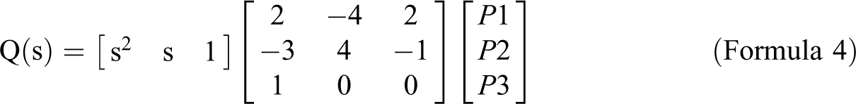
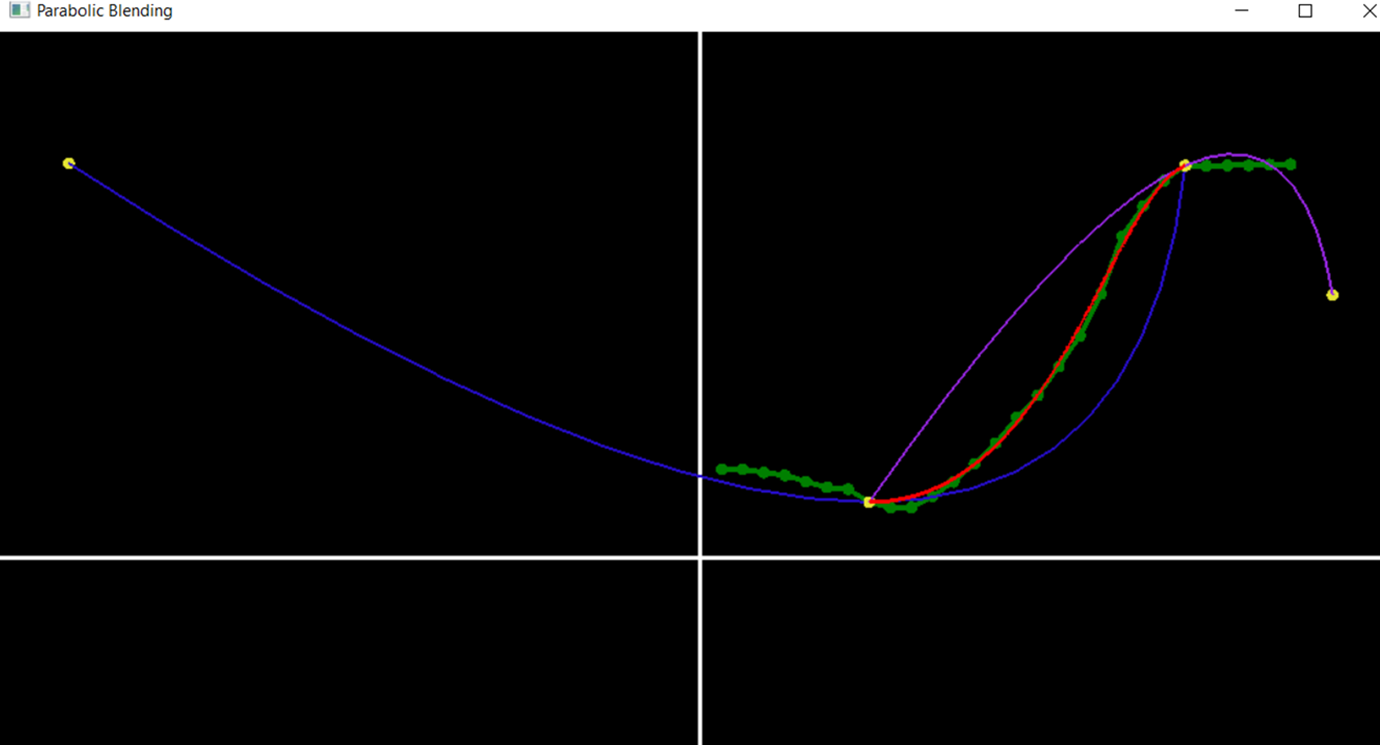
In the most general sense, the process of creating a cubic between two parabolas is called parabolic blending.^21,22 Three vertices are selected from four control vertices (P₁–P₄) to form two parabolas (Figure 4). P₁, P₂ and P₃ define the P(r) parabola, while P₂, P₃ and P₄ define the Q(s) parabola.

Figure 4.

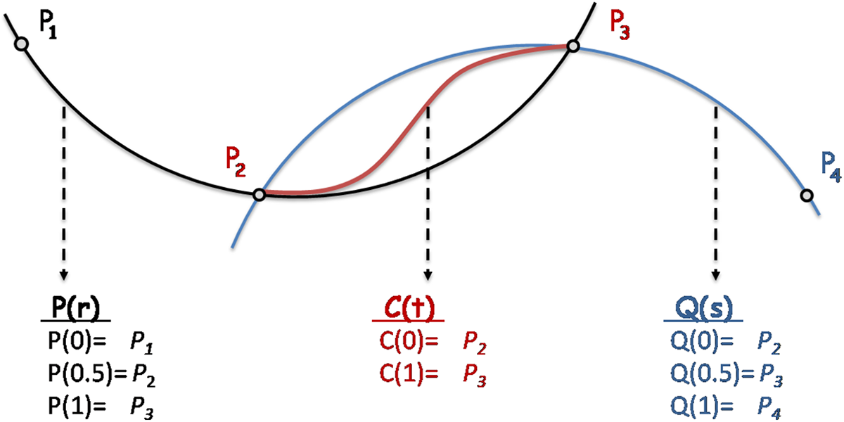
Parabolas and control vertices that define PB.

The C(t) curve is defined, with the intersection vertices of the parabolas P(r) and Q(s), the vertices P₂ and P₃, the starting and ending points. The definition of the C(t) curve is called PB, with the creation of a third-order equation that includes the P(r) and Q(s) parameters.

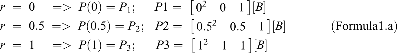
When calculating the values of P(r), r parameter was used (0 ≤ r ≤ 1). Since a parabola is defined, P(r) is a second order equation (Formula 1).

P (r) = [\begin{matrix} r^{2} & r & 1 \end{matrix}] [\begin{matrix} B \end{matrix}]

Formula\ 1

When creating the equation for P(r), selected control vertices are taken as reference points (Figure 4). Formula 1.a is obtained when reference values are opened for control vertices. Here [B] will form the coefficient matrix, and it is created depending on the control points.

\begin{array}{l} r = 0 = > P (0) = P_{1}; P 1 = [\begin{matrix} 0^{2} & 0 & 1 \end{matrix}] [B] \\ r = 0.5 = > P (0.5) = P_{2}; P 2 = [\begin{matrix} {0.5}^{2} & 0.5 & 1 \end{matrix}] [B] \\ r = 1 = > P (1) = P_{3}; P 3 = [\begin{matrix} 1^{2} & 1 & 1 \end{matrix}] [B] \end{array}

Formula 1.a

Formula 1.b occurs when Formula 1.a is combined to the side.

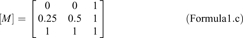
[\begin{matrix} P 1 \\ P 2 \\ P 3 \end{matrix}] = [\begin{matrix} 0 & 0 & 1 \\ 0.25 & 0.5 & 1 \\ 1 & 1 & 1 \end{matrix}] [B]

Formula 1.b

If the matrix that creates the r values for the selected control points is called [M], Formula 1.c occurs.

[M] = [\begin{matrix} 0 & 0 & 1 \\ 0.25 & 0.5 & 1 \\ 1 & 1 & 1 \end{matrix}]

Formula 1.c

If the coefficient matrix is drawn from the equation, Formula 1.d is created (if Formula 1.c is replaced in Formula 1.b).

[\begin{matrix} P 1 \\ P 2 \\ P 3 \end{matrix}] = [M] [B]

Formula 1.d

If [B] is left alone in Formula 1.d, Formula 1.e is obtained.

[B] = {[M]}^{- 1} [\begin{matrix} P 1 \\ P 2 \\ P 3 \end{matrix}]

Formula\ 1.e

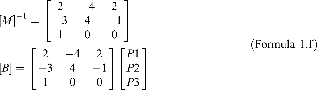
If the inverse ([M]⁻¹) of [M] is taken, instead of the matrix in Formula 1.e, Formula 1.f occurs.

\begin{array}{l} {[M]}^{- 1} = [\begin{matrix} 2 & - 4 & 2 \\ - 3 & 4 & - 1 \\ 1 & 0 & 0 \end{matrix}] \\ [B] = [\begin{matrix} 2 & - 4 & 2 \\ - 3 & 4 & - 1 \\ 1 & 0 & 0 \end{matrix}] [\begin{matrix} P 1 \\ P 2 \\ P 3 \end{matrix}] \end{array}

Formula\ 1.f

If Formula 1.f is substituted in Formula 1, which is the main formula, Formula 2 is obtained for the representation of P(r) parabola with 3 control vertices (P_1–3).

P (r) = [\begin{matrix} r^{2} & r & 1 \end{matrix}] [\begin{matrix} 2 & - 4 & 2 \\ - 3 & 4 & - 1 \\ 1 & 0 & 0 \end{matrix}] [\begin{matrix} P 1 \\ P 2 \\ P 3 \end{matrix}]

Formula\ 2

When calculating the values of Q(s), s parameter was used (0 ≤ s ≤ 1). In this case, the parametric equation for Q(s) is obtained in the same way as the path followed when calculating P(r) (Formula 2).

Q (s) = [\begin{matrix} s^{2} & s & 1 \end{matrix}] [D]

Formula\ 3

Formula 4 is obtained when the processes from Formula 1 to the derivation of Formula 2 are repeated for three control vertices (P_2–4). The control vertices in P(r) and Q(s) are different from each other (Figure 4).

Q (s) = [\begin{matrix} s^{2} & s & 1 \end{matrix}] [\begin{matrix} 2 & - 4 & 2 \\ - 3 & 4 & - 1 \\ 1 & 0 & 0 \end{matrix}] [\begin{matrix} P 1 \\ P 2 \\ P 3 \end{matrix}]

Formula\ 4

C (t) intersects at vertices P(r) and Q(s) with P₂ and P₃, as can be seen in Figure 4. Two separate line equations can be defined for these two points (Formula 5, Formula 6).

r = k_{1} * t + k_{2}

Formula\ 5

Formula 5.a is obtained when coefficients are accumulated for a line equation for points P₂ and P₃, which are the intersection of C(t) with P(r).

For P(r);

\begin{array}{l} P_{2} : r = 0.5; t = 0 => r = k_{1} * t + k_{2} \\ 0.5 = k_{1} * 0 + k_{2} => k_{2} = 0.5 \\ P_{3} : r = 1; t = 1 => r = k_{1} * t + k_{2} \\ 1 = k_{1} * 1 + 0.5 => k_{1} = 0.5 \end{array}

r (t) = 0.5 * t + 0.5

Formula\ 5.a

For Q(s);

s = k_{3} * t + k_{4}

Formula\ 6

Formula 6.a is obtained when coefficients are accumulated for a line equation for points P₂ and P₃, which are the intersection of C(t) with Q(s).

\begin{array}{l} P_{2} : s = 0; t = 0 = > s = k_{3} * t + k_{4} \\ 0 = k_{3} * 0 + k_{4} = > k_{4} = 0 \\ \begin{array}{l} P_{3} : s = 0.5; t = 1 = > s = k_{3} * t + k_{4} \\ 0.5 = k_{3} * 1 + 0 = > k_{3} = 0.5 \end{array} \end{array}

s (t) = 0.5 * t

Formula\ 6.a

The C (t) curve is affected by P(r) and Q(s). The weight of the t parameter is calculated depending on the r and s parameters. Formula 5.a and Formula 6.a are replaced by Formula 2 and Formula 4 respectively, and Formula 7, the resulting equation for C(t), is obtained.

C (t) = (1 - t) P (r) + t Q (s)

Formula\ 7

Formula 7 creates the result equation to be used to draw C(t) (0 ≤ t ≤ 1) (Figure 4).

Software interface design

In this section, the development stages of the interface design to be used to estimate the thickness distributions of the PS samples at regular intervals by using the PB method are given.

The linear spaced measurement values (green dots, line is created by connecting the dots) obtained from the 3 mm thick sheet are shown in Figure 5 (X- linear measurement ranges, Y-thickness). In this way, the yellow dots represent the control vertices sequentially (P_1–4). C(t) (red line) between P(r) (blue line) and Q(s) (purple line) significantly overlaps with the thickness distribution curve being measured.

Figure 5.

PB process for measuring the values of thermoformed samples with a thickness of 3 mm.

Parameters for the values produced by the developed interface for the C(t) curve with measurement values of the thermoformed sample with a thickness of 3 mm are shown in Table 3.

Table 3.

PB curve values (C(t)) for measured thickness values from the thermoformed sample with a thickness of 3 mm and selected control vertices.

Measuring Points	X axis values	Y axis values		Error
Measuring Points	X axis values	Measured thickness value (mm)	Y axis value produced by the program, C(t)	Error (mm)	Relative error	Relative error (%)
8	0.8	0.428	0.4283	0.0000	0.0000	0.0
9	0.9	0.386	0.4381	0.0515	0.1332	13.3
10	1	0.388	0.4694	0.0811	0.2089	20.8
11	1.1	0.471	0.5244	0.0528	0.1120	11.1
12	1.2	0.581	0.6055	0.0239	0.0411	4.1
13	1.3	0.718	0.7153	−0.0030	−0.0042	−0.4
14	1.4	0.876	0.8563	−0.0203	−0.0232	−2.3
15	1.5	1.070	1.0312	−0.0388	−0.0363	−3.6
16	1.6	1.238	1.2418	0.0035	0.0028	0.2
17	1.7	1.456	1.4881	0.0315	0.0216	2.1
18	1.8	1.690	1.7668	0.0768	0.0454	4.5
19	1.9	2.010	2.0677	0.0577	0.0287	2.8
20	2	2.448	2.3712	−0.0771	−0.0315	−3.1
21	2.1	2.675	2.6472	−0.0278	−0.0104	−1.0
22	2.2	2.868	2.8607	−0.0076	−0.0026	−0.2
23	2.3	2.983	2.9833	0.0000	0.0000	0.0

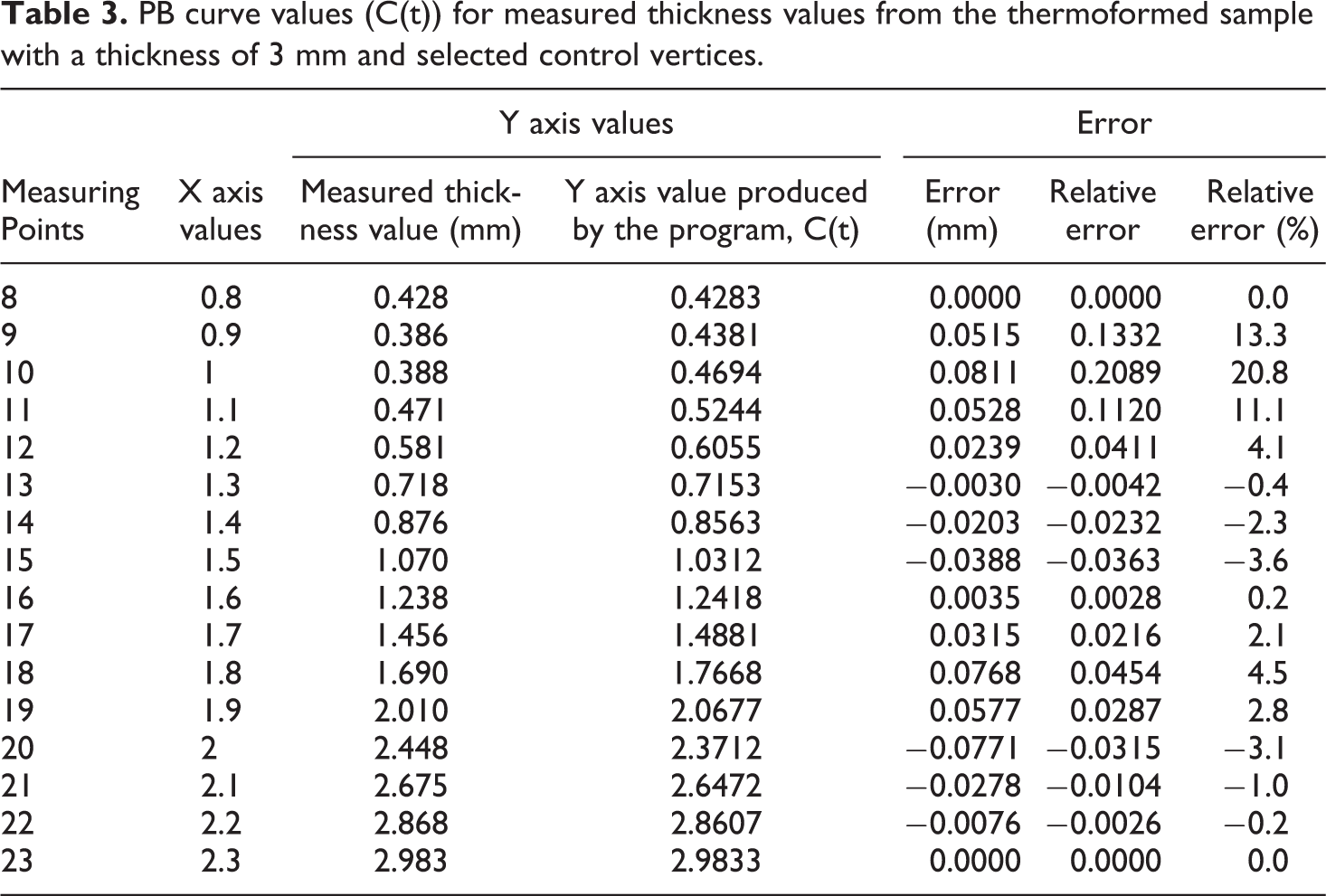
While the measurement values are shown for the sheet, each measurement in the x-axis is linearly created in an ascending order with 0.1 precision. For example, the 3rd measurement value parameters are given as (X, Y) – (0.3, Y_0.3), whereas the 19th measurement values are given as (X, Y) – (1.9, Y_1.9). Table 3 shows the results produced by the program for each measured point. The error, relative error and percentage relative error values are listed. For the 15th (n) point the error is −0.0388 (X_n − X’_n), the relative error is −0.0363 ((X_n − X’_n)/X_n) and the relative error (percentage) is −3.6% (((X_n − X’_n)/X_n) * 100). Absolute values of the errors were not taken to facilitate the follow-up of whether the error occurred in a negative or positive direction for the points where the measurement and estimation was made. The total absolute percentage relative error value was calculated as 70.1856 ( $\sum_{n = 8}^{23} |r e l a t i v e p e r c e n t a g e e r r o r|$ ) and the average absolute percentage relative error value was calculated as 4.3866 (( $\sum_{n = 8}^{23} |r e l a t i v e p e r c e n t a g e e r r o r|$ )/16).This value means that the program has produced a highly accurate result for this study.

Create a pattern

Up to this stage, the PB process has been performed for values that were obtained from thermoformed samples at a thickness of 3 mm. Selected control vertices determine the characteristic of the curve created in the PB process. The control vertices are determined in such a way that they can create a pattern for the sheet to be used in the next step (estimation of thickness values for thermoformed samples at a thickness of 1.25 mm). The control vertices selection criteria for the 3 mm sheet are shown in Table 4.

Table 4.

Selection criteria for PB control vertices for the 3 mm mould.

Control Vertices	Axis	Values	Criteria
P₁	x	−3	(−) marked sheet thickness value
P₁	y	3	Initial sheet thickness value
P₂	x	0.8	Marginal slope point x value in the direction of the base of sample
P₂	y	0.4283	Marginal slope point y value in the direction of the base of sample
P₃	x	2.3	Marginal slope point x value in the direction of the top of sample
P₃	y	2.9833	Marginal slope point y value in the direction of the top of sample
P₄	x	3	X axis measurement limit point
P₄	y	2	Y axis limit point for drawing Q(s) (estimated choice)

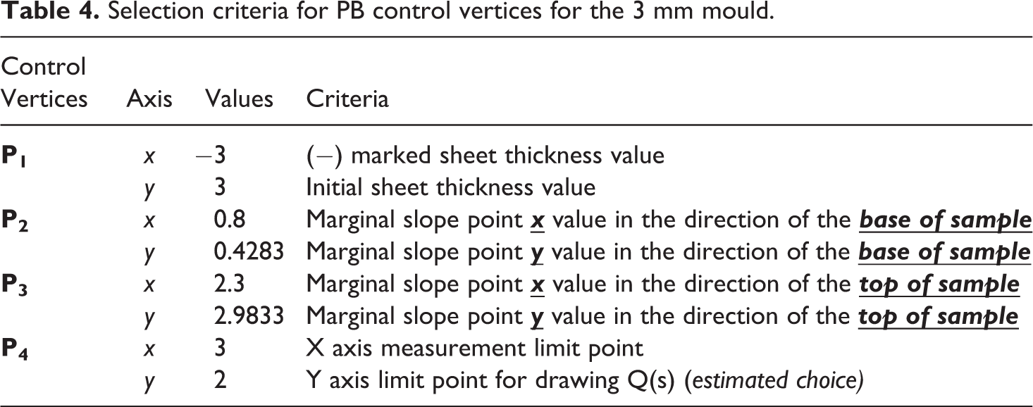
The P₄ x axis value is the linear value limit taken from the sheet. The P₄ y-axis value has been selected as an estimate to define the Q(s) curve taking into account the P₄ x-axis value (Table 4). A pattern is defined between the control vertices selected for the 3 mm sheet and the control vertices that will be selected for the 1.25 mm sheet, whose values will be estimated. This pattern and the control vertices values to be assigned in the program for the 1.25 mm sheet are shown in Table 5.

Table 5.

Control vertices values for sheets with a thickness of 1.25 mm, determined using the pattern.

Pattern for the selection of sheet control vertices
Calculated values for 1.25 mm thick sheet				Algorithm
Calculated values for 1.25 mm thick sheet				# (steps)	Processes
P₁	x	−1.25	(−) marked sheet thickness value	1	Advance in the −x direction until the sheet thickness value
P₁	y	1.25	Initial sheet thickness value	2	Get initial sheet thickness value
P₂	x	0.8	Marginal slope point x value in the direction of the base of sample	3	Set measurement value with 8 rows as the first marginal slope point
P₂	y	0.161	Marginal slope point y value in the direction of the base of sample	4	Multiply the ratio by measuring number 8 with a thickness of 3 mm (sheet thickness/3); $0.3866 * (1.25 / 3) = 0.1610$
P₃	x	2.3	Marginal slope point x value in the direction of the top of sample	5	Set measurement number 23 as the second marginal slope point
P₃	y	1.243	Marginal slope point y value in the direction of the top of sample	6	Multiply the ratio of the number 23 with the thickness of 3 mm (sample thickness/3); $2.9833 * (1.25 / 3) = 1.243$
P₄	x	3	X axis measurement limit point	7	Get X axis measurement limit point value
P₄	y	0.8333	Y axis limit point for drawing Q(s) (estimated choice)	8	Multiply the ratio of 3 mm thickness P₄ y axis by (sample thickness/3); $2 * (1.25 / 3) = 0.8333$

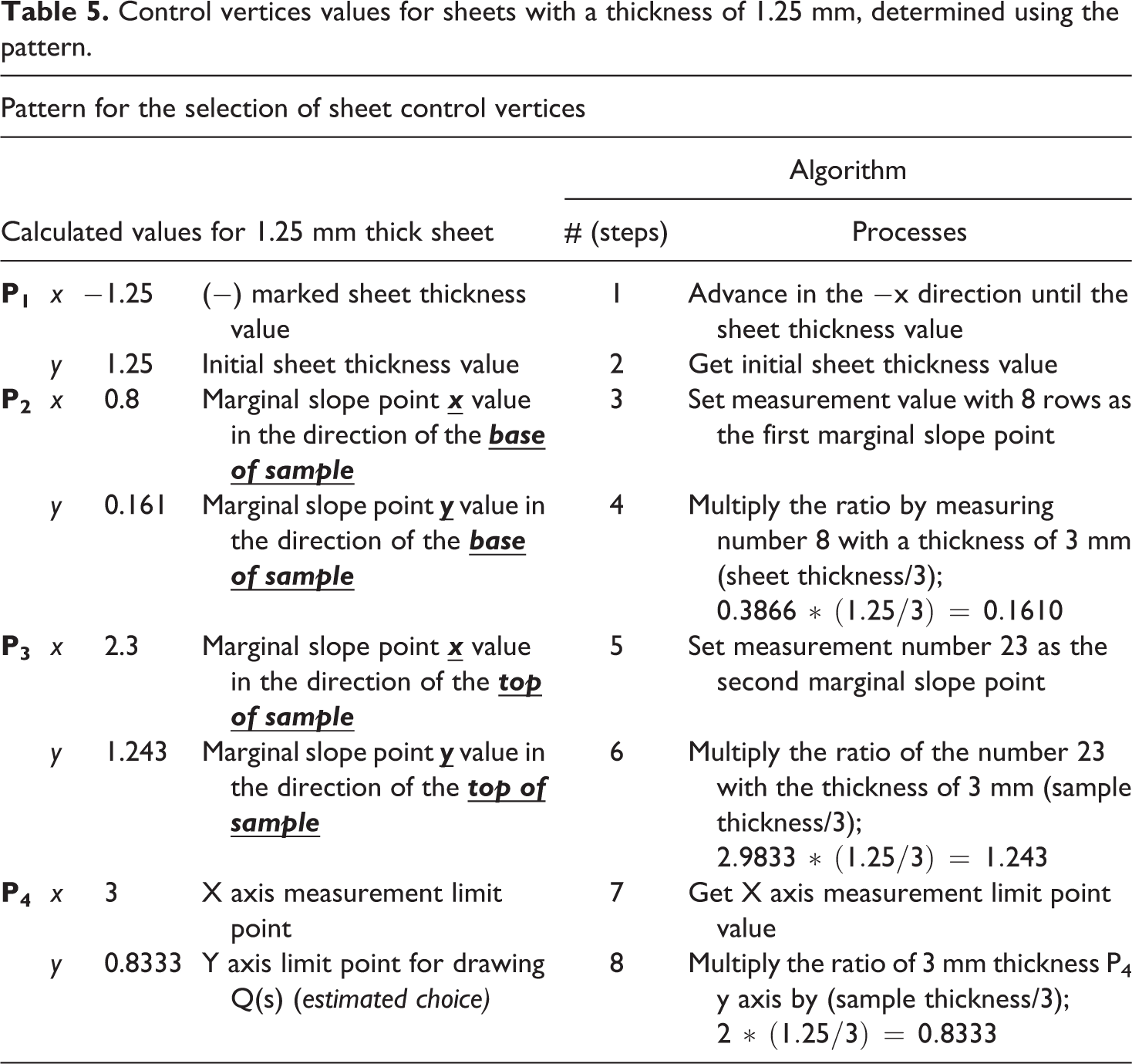
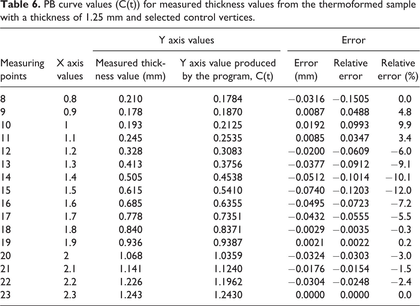
Table 6 shows the results produced by the program for each measured point. The error, relative error and percentage relative error values are listed. The total absolute percentage relative error value was calculated as 91.1132, and the average absolute percentage relative error value was calculated as 5.6945.

Table 6.

PB curve values (C(t)) for measured thickness values from the thermoformed sample with a thickness of 1.25 mm and selected control vertices.

Measuring points	X axis values	Y axis values		Error
Measuring points	X axis values	Measured thickness value (mm)	Y axis value produced by the program, C(t)	Error (mm)	Relative error	Relative error (%)
8	0.8	0.210	0.1784	−0.0316	−0.1505	0.0
9	0.9	0.178	0.1870	0.0087	0.0488	4.8
10	1	0.193	0.2125	0.0192	0.0993	9.9
11	1.1	0.245	0.2535	0.0085	0.0347	3.4
12	1.2	0.328	0.3083	−0.0200	−0.0609	−6.0
13	1.3	0.413	0.3756	−0.0377	−0.0912	−9.1
14	1.4	0.505	0.4538	−0.0512	−0.1014	−10.1
15	1.5	0.615	0.5410	−0.0740	−0.1203	−12.0
16	1.6	0.685	0.6355	−0.0495	−0.0723	−7.2
17	1.7	0.778	0.7351	−0.0432	−0.0555	−5.5
18	1.8	0.840	0.8371	−0.0029	−0.0035	−0.3
19	1.9	0.936	0.9387	0.0021	0.0022	0.2
20	2	1.068	1.0359	−0.0324	−0.0303	−3.0
21	2.1	1.141	1.1240	−0.0176	−0.0154	−1.5
22	2.2	1.226	1.1962	−0.0304	−0.0248	−2.4
23	2.3	1.243	1.2430	0.0000	0.0000	0.0

Results and discussions

The thickness distributions for all of the thickness cases are shown in Figure 3. The results, as shown in Figure 3, indicate that five of the thickness distribution curves show nearly the same variation trend along the measuring points. One of the purposes of this research is to create the appropriate mathematical functions for thickness distribution curves in Figure 3. For this reason, PB was chosen for fitting curves that are most likely to match each thickness distribution curve.

As seen in Figure 3, the minimum thickness value was measured as 0.133, 0.113, 0.193, 0.173 and 0.388 mm in Point 10, for the thermoformed samples with initial thicknesses of 0.9, 1, 1.25, 1.3 and 3 mm respectively. Point 10 is in the base corner of the thermoformed sample, where the PS sheet last touched the mould during the forming. The maximum thickness values were obtained for all of the thickness cases from Points 23 to 28. These points are located from the top corner of the thermoformed sample to the edge. From the data in Figure 3, it can be seen that the thickness did not change significantly from Points 1 to 8 and from Points 23 to 28. Therefore, PB was applied especially from Points 8 to 23.

On the other hand, the temperature distribution on the heated PS sheet is one of the factors that affects the thickness distribution of a thermoformed sample. This phenomenon can clearly be seen in Figures 6 and 7. To show the nonlinear temperature distribution on the heated sheet before thermoforming, temperature distribution was examined along some preselected directions using software from Testo. Figures 6 and 7 indicate that the temperature values are quite different from each other in the P1, P2, P3 and P4 directions. For an effective thermoforming operation, the temperature should not change by more than 5°C in the selected direction. The temperature value should remain almost the same at every point. This is important for particularly semi-crystalline polymers such as Polypropylene and Polyethylene. PS, which was thermoformed in this study, is an amorphous thermoplastic, therefore it can be thermoformed in wide temperature ranges. As shown in Figure 6, the maximum and minimum temperature values that were measured in the selected directions are quite different. From Figure 7 it is possible to observe the same trend as in Figure 6. From Figure 7, at some points in the P1 and P2 directions, which are perpendicular to each other, the temperature difference is greater than 20°C. In summary, these results indicate that for a heated PS sheet before thermoforming, if the temperature is higher in some regions, it deforms more easily and is affected by biaxial stretching more significantly than the other regions. For this reason, non-uniform wall thicknesses occur in the thermoformed samples.

Figure 6.

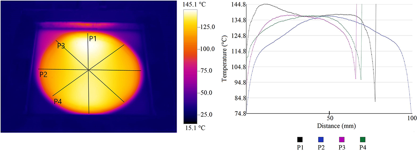
Comparison of temperature distribution along selected directions for PS sheets with an initial thickness of 1.25 mm.

Figure 7.

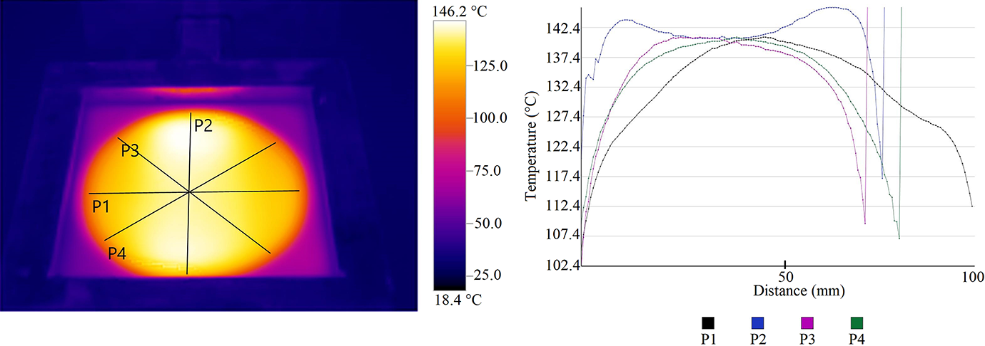
Comparison of temperature distribution along selected directions for PS sheets with an initial thickness of 3 mm.

In this study, PB was used for the first time to estimate the thickness distribution of a thermoformed sample. Table 3 shows the measured and estimated thickness values with errors in a thermoformed sample with a thickness of 3 mm. From Table 3, it is understood that the estimated thickness values are in good agreement with those measured. From Table 3, although the thickness was measured as 0.388 mm at Point 10, it was estimated as 0.469 mm. Point 10 is the point at which the minimum thickness value occurs in the thermoformed sample. Moreover, the thickness was estimated with the highest error value (20.8859%) at Point 10. Except for Point 10, all of the estimated values have an acceptable error value for thermoforming. Additionally, Table 6 shows the estimated thickness values for thermoformed samples with a thickness of 1.25 mm. The highest error value is 12.0%, at Point 15. Thickness was measured as 0.615 mm at Point 15, but it was estimated as 0.541 mm. Point 15 is located at the sidewall of the thermoformed sample. Other thickness values were estimated as having an acceptable margin of error (<10%). Furthermore, Figure 8 shows the estimated and measured thickness distributions for the thermoformed samples with initial thicknesses of 1.25 and 3 mm graphically. Also, it can be seen that the estimated thickness values are quite close to those measured in Figure 8.

Figure 8.

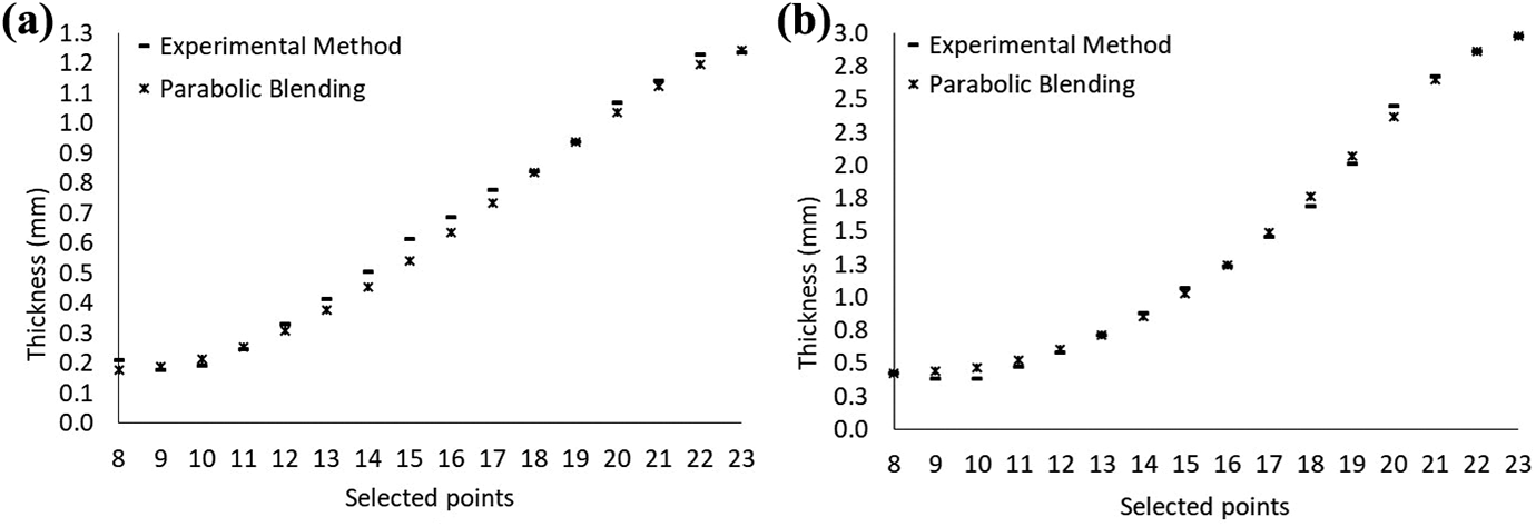
Comparison of measured and estimated thickness distributions for thermoformed samples with an initial thickness of a) 1.25 mm b) 3 mm.

Conclusion

If mass production is possible in thermoforming, thickness distribution is obtained for only a few samples among thousands of thermoformed samples. Furthermore, thickness detection is a destructive and time-consuming process. Especially for food packaging using thermoforming, thousands of packages can be produced in a production line with the same mould. To use production time efficiently, and to detect the thickness distribution of produced samples nondestructively, PB has been investigated as an alternative method in this work. A pattern was created regarding the control vertices that should be chosen to perform the PB process for the moulds used. The extracted pattern is shown using a computer graphics based program. Using PB, thickness distributions were estimated for thermoformed samples with thicknesses of 1.25 and 3 mm. Thickness values estimated using PB are in good agreement with those values measured. At only a few points, the relative error in the estimated values was greater than 10%. Since PB was being used for the first time in thickness estimation in thermoforming, less than 10% relative error can be considered reasonable. In this investigation, the goal was to assess the efficacy of PB in the estimation of the thickness distribution of thermoformed samples. A further study with more focus on the accuracy of PB should be done to estimate the thickness distribution of thermoformed samples precisely. Additionally, alternative non-destructive methods such as image processing should be used in the estimation of the thickness distribution of thermoformed packages.

Footnotes

Declaration of conflicting interests

The author(s) declared no potential conflicts of interest with respect to the research, authorship, and/or publication of this article.

Funding

The author(s) received no financial support for the research, authorship, and/or publication of this article.

ORCID iD

Olcay Ekşi

References

Throne

. Thermoforming. Munich: Hanser, 1987.

Throne

. Technology of thermoforming. Cincinnati, OH: Hanser/Gardner, 1996.

Klein

. Fundamentals of plastics thermoforming. San Rafael, CA: Morgan & Claypool, 2009.

Throne

. Understanding thermoforming. Cincinnati, OH: Hanser/Gardner, 2008.

Moustafa

Dotchev

Wells

, et al. Investigation of thermoforming tool design and pocket quality. J Therm Eng 2015; 1: 670–676.

Sasimowski

. A pressure-bubble vacuum forming process for polystyrene sheet. Adv Sci Tech 2017; 11: 180–186.

Jobey

Allanic

Mousseau

, et al. Prediction of thickness distribution of thermoformed multilayer ABS/PMMA sheets. In: The 19th international ESAFORM conference on material forming – ESAFORM 2016, Nantes, France, April 2016, pp. 170033–60016.

Sarakhun

Tamna

Thammakornbunjut

. Finite element analysis of plastic cups. In: 118th IASTEM international conference, Bangkok, Thailand, 5–6 June 2018, pp. 92–94.

Study on thickness distribution of thermoformed medical PVC blister. In: 2nd International conference on materials science, energy technology and environmental engineering (MSETEE 2017), Zhuhai, China, 28–30 April 2017, pp. 1–7.

10.

Modławski

Jaruga

. Computer simulation of thermoforming process and its verification using a rapid tooling mould. In: MATEC Web of Conferences, Częstochowa, Poland, 14 March 2018, pp. 1–10.

11.

Leite

Rubio

JCC

Cabrera

, et al. Vacuum thermoforming process: an approach to modeling and optimization using artificial neural networks. Polymers 2018; 10: 143–159.

12.

Beilharz

Bonten

Eyerer

. Influence of processing conditions on the thermoformability of PP-sheet material. In: SPE annual technical conference, Massachusetts, USA, 1–5 May 2011, pp. 2504–2508. New York: Curran.

13.

Seefried

Drummer

. The effects of radiation cross-linking and process parameters on the behavior of polyamide 12 in vacuum thermoforming. Polym Eng Sci 2012; 52: 884–892.

14.

Gunel

Başaran

. Micro-deformation mechanisms in thermoformed alumina trihydrate reinforced poly(methyl methacrylate). Mater Sci Eng A 2009; 523: 160–172.

15.

Molnar

Ogale

Lahr

, et al. Influence of drapability by using stitching technology to reduce fabric deformation and shear during thermoforming. Compos Sci Technol 2007; 67: 3386–3393.

16.

Cabrera

Reynolds

Alcock

, et al. Non-isothermal stamp forming of continuous tape reinforced all-polypropylene composite sheet. Compos Pt A 2008; 39: 1455–1466.

17.

Alcock

Cabrera

Barkoula

, et al. Low velocity impact performance of recyclable all-polypropylene composites. Compos Sci Technol 2006; 66: 1724–1737.

18.

Gunel

Basaran

. Stress whitening quantification of thermoformed mineral filled acrylics. J Eng Mater Technol 2010; 132: 031002 (11 pages).

19.

Chung

Kim

Ryu

, et al. Sound generation and radiation from rotor tip-vortex pairing phenomenon. AIAA J Air Transp 2006; 44: 1181–1187.

20.

Kunz

Stilman

. Time-optimal trajectory generation for path following with bounded acceleration and velocity. In: Roy

Newman

Srinivasa

(eds) Robotics: science and systems VIII. Cambridge, MA: The MIT Press, 2013, pp. 209–216.

21.

Hadavinia

Travis

Fenner

. C1-continuous generalised parabolic blending elements in the boundary element method. Math Comput Model 2000; 31: 17–34.

22.

Rogers

Adams

. Mathematical elements for computer graphics. 2nd ed. New York: McGraw-Hill, 1989.