
Abstract
A 3-DOF (degree of freedom) planar motion motor using multiple linear motors as actuators is widely implemented in ultra-precision positioning systems. It is a multi-input multi-output (MIMO) system and requires an accurate decoupled model for controller design. In practice, there are modelling errors between the nominal model and the actual model, such as the force ripple, inhomogeneous air-gap thickness, measurement noise and uncertain disturbances. Due to the modelling errors, this MIMO system cannot be decoupled and the desired tracking performance specifications will not be achieved. In order to improve the servo performance of the planar motor with uncertainties, a non-linear composite controller consisting of u1 and u2 terms is proposed. u1 is designed to compensate for the modelling errors; therefore the coupling effects between multi-degrees of freedom are reduced and the robustness is improved. In order to reduce the large servo error amplitudes, which are caused by the low-frequency disturbances and high-frequency noise, an amplitude-based variable-gain function is applied in u2; thus the control action benefits from this operation by suppressing the low-frequency contribution and no extra control effect, to avoid the high-frequency noise. The convergence and stability of the control law are guaranteed by Lyapunov stability theory. The trajectory tracking experimental results show that the proposed control method has superior tracking performance and positioning ability compared with the well-known inverse dynamics controller. This indicates that the non-linear composite controller is an attractive approach to improve the servo performance of a system with uncertainties.
Keywords
Introduction
Due to the ever increasing performance requirements in many accurate positioning systems, e.g. semiconductor scanners, LCD and inspection systems, precision stages using a non-contact linear actuator mainly based on magnetic forces have been developed (Boeij, 2006; Cho, 2002; Cornelis, 2008; Gao et al., 2003; Hu Tiejun, 2006; Jansen, 2007a, 2007b, 2008; Jung and Baek, 2003; Kim and Trumper, 1998). However, the task of obtaining even higher accuracy with conventional XY stages combined with a linear motor and ball screws has reached its limitations. During the last decade, planar motion stages with the capability of multi-degree of freedom (DOF) motion have been developed as alternatives to the XY drivers. Usually, a planar motor is actuated by multiple linear motors and supported by air bearings. The main benefits include direct drive, high force density, the miniaturization of structure, and most importantly, the capability of high positioning accuracy and high speed with the assistance of well-developed position sensor technologies such as laser interferometers. Therefore, planar motors are widely used in ultra-precision positioning semiconductor manufacturing equipment, and especially its motion control systems used on the wafer stage.
A 3-DOF planar motor is a MIMO system and the commonly used control method is the well-known inverse dynamics-based controller (Mistry et al., 2010; Tar et al., 2009; Wang and Xie, 2009). However a drawback to the implementation of this control methodology is that the parameters of the system must be known exactly. In practice, a real system cannot be described accurately enough due to the disturbance and parametric uncertainties; as a result, an actual model of the system cannot be obtained. Indeed, any model is inherently only an approximation of reality, so only a nominal model is obtained. The dynamics modelling and the controller design are all based on this simplified nominal model, and therefore modelling errors exist between the nominal model and actual model. For a planar motor, the modelling errors include: 1) the Lorentz force errors caused by the manufacturing errors of permanent magnets and coils; 2) only the fundamental component of the analytical expression of the magnetic field, and the higher-order harmonic components are ignored; 3) the coil shape is simplified as linear; 4) the air-gap thickness is not uniform, and therefore the magnetic field along the Z-axis changes in the index; 5) force ripple; 6) measurement noise; 7) un-modelled high frequency dynamics; 8) damping friction force; 9) external cable disturbances; and 10) the output current errors of the driver. Due to the modelling errors, which are coupling, time-varying and non-linear, the uncertain MIMO system cannot be decoupled as a single-input single-output (SISO) system by the inverse dynamics-based controller, which is a case of the method of feedback linearization. Moreover, the right side of the error equation of the closed-loop system is not zero; therefore the convergence of the tracking errors is no longer guaranteed and the ideal tracking performance is not satisfied.
On the other hand, the low-frequency disturbances cause large servo error amplitudes, whereas high-frequency disturbances induce small servo error amplitudes. Therefore, the servo performance achieved with linear control and standard feedforward design is no longer satisfactory. This is partly due to the inherent linear design limits encountered under linear feedback. Namely, if the error response contains frequency contributions sufficiently below the controller bandwidth, then the servo performance benefits from an increased controller gain; beyond the bandwidth, extra controller gain often induces the amplification of noise. This is the classical result obtained from Bode’s Sensitivity Integral (Freudenberg et al., 2000). Monitoring the servo error signals at hand and acting accordingly, the choice for a dynamic controller gain can significantly improve upon servo performance (Arcak et al., 2003; Freudenberg et al., 2003).
In order to improve the tracking performance of the planar motors with uncertainties, a non-linear composite controller is proposed in this paper; thus the stability of this control law is proved by Lyapunov theory. The proposed non-linear strategy basically has two terms u1 and u2. The function u1 is used to compensate for the modelling errors, then the effects of the coupling between multi-degrees of freedom are reduced and the robustness accordingly enhanced. The action u2 applies to variable controller gains mostly on the basis of the amplitude information of the error signals at hand. This operation induces a high gain to suppress the low-frequency contribution and low-gain feedback to avoid the effect of the high-frequency noise amplification. Trajectory tracking experimental results show that the servo performance and the robustness of the system are greatly improved.
This paper is organized as follows: the next section presents the decoupled dynamic force–current model of the planar motor. Then, the stability and the servo performance of the system with uncertainties obtained by the inverse dynamics-based linear controller are discussed. The detailed non-linear composite control algorithm and the stability proved by Lyapunov theory are introduced, followed by the trajectory tracking experimental results confirming the effectiveness of the overall control strategy. Finally, conclusions are drawn in the last section.
Force–current decoupled model
Dynamics of planar motor
Figure 1 shows a photograph of the 3-DOF planar motor discussed in this paper, and a schematic of this stage is shown in Figure 2. The Halbach permanent magnet array is applied as the stator, and part of the magnetic field distribution is shown in Figure 3. The rotor comprises four linear motors, a coil skeleton, four air bearings and two mirrors for the laser that senses positions. The XYθz planar motion is realized through the four linear motors and air bearings. Each linear motor consists of three coils. Taking linear A as example, the coil size and the magnetic pole distance are shown in Figure 4. The driver drives the electrical current of the coils and controls the motor position according to the positioning command from a host controller. As shown in Figure 5, linear motor A and linear motor B generate X-direction driving force, linear motor C and linear motor D exert Y-direction driving force, and the difference among these forces produces the torque about Z-axis. The three-axis laser interferometer senses the Y1, Y2 and X positions, the distance between Y1 and Y2 is l=28 mm. The signal of Y1 and Y2 sensed position are converted into Y coordinates, i.e. Y=(Y1+Y2)/2. The angle around about the Z axis θz is calculated from the difference between Y1 and Y2 positions, i.e. θz=(Y1−Y2)/l.
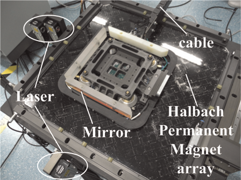
Photograph of the 3-DOF planar motor.
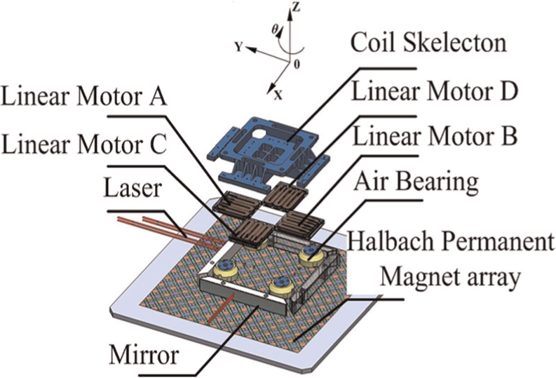
Schematic of the 3-DOF planar motor.
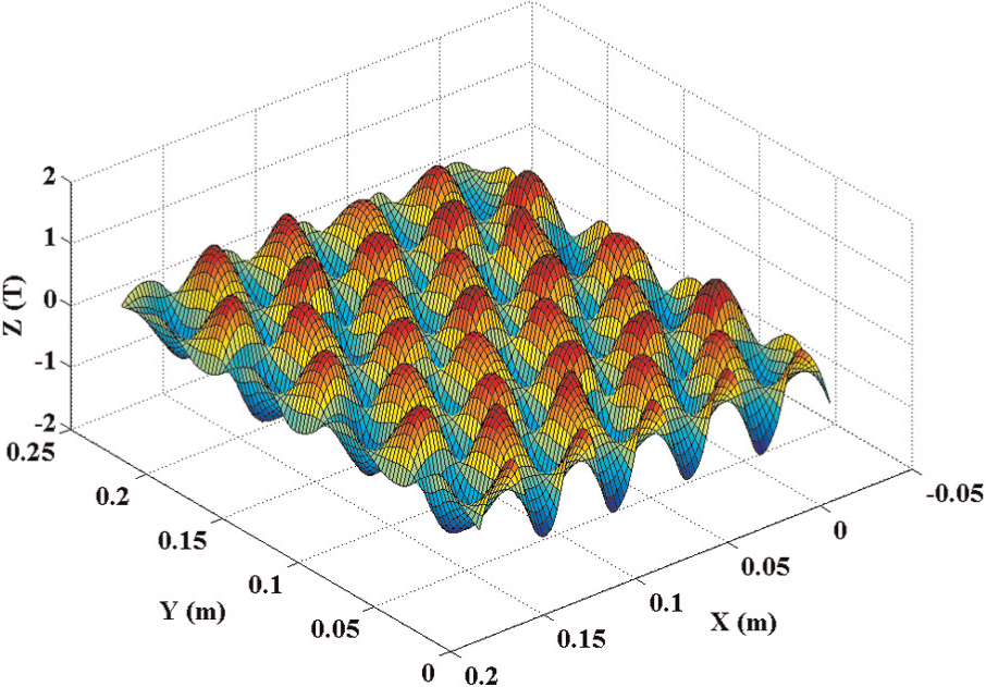
The magnetic field of the Halbach permanent magnet array.

Coil size.
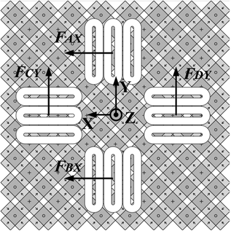
The drive forces generated by linear motor.
The dynamics of the planar motor is obtained by the Lagrange method as
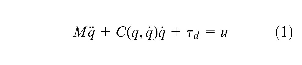
where
The servo drivers control the position on the X, Y and θz axis independently when converting the position signals into commands to be sent to the A, B, C and D linear motors, i.e.
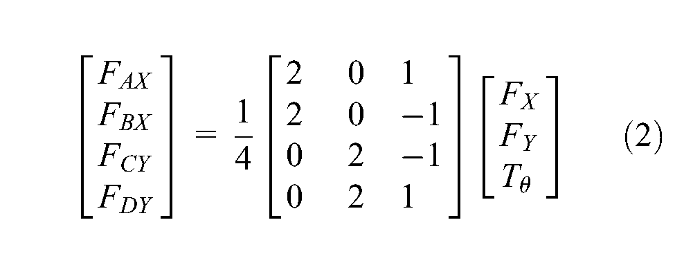
where F AX , F BX , F CY and F DY are the driving forces generated by the linear motors A, B, C and D respectively, as shown in Figure 5.
Current distribution
The dq0 method (Kim and Trumper, 1998) is applied for the current distribution in any linear motor. Taking the linear motor A as an example, its structural configuration is shown in Figure 6.
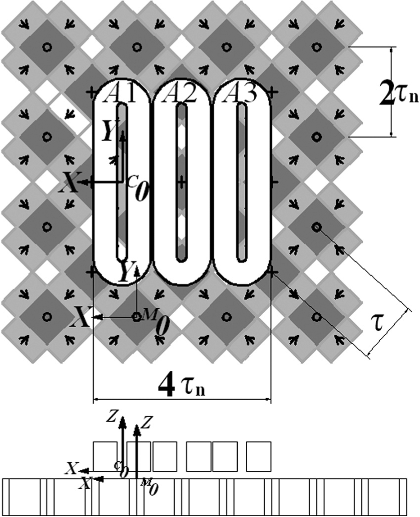
Structural configuration of the linear motor A.
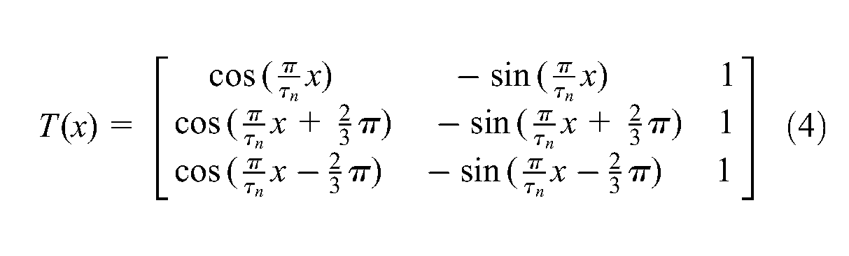
The linear motor A consists of three coils named A1, A2 and A3, respectively. According to the coordinate system defined in Figure 6, whose origin is at the surface centre of the N pole of a magnet and the bottom centre of coil A1, respectively, the transition arithmetic between the currents and the X-direction force exerted by the three coils can be expressed as:
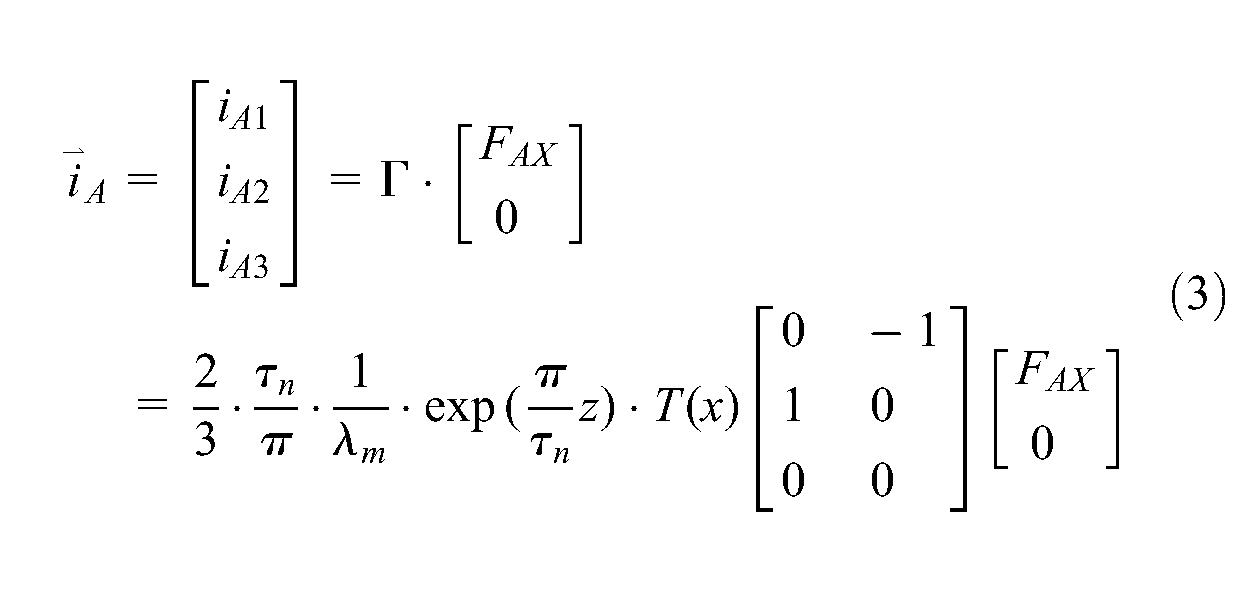
where iAi is the current in coil Ai, FAx is the X-direction force exerted by linear motor A, τ is the permanent magnet array pitch and
Note that, according to Equations (2) and (3), the relationship between all the forces/torque and the coil currents are established and it provides a force–current decoupled model for controller design.
Non-linear composite control
Coupling effects caused by modelling errors
According to Equation (1), the planar motor is a MIMO system and the well-known inverse dynamics control method can be applied. However, a drawback to the implementation of this method is that the parameters of the system must be known exactly. In practice, there are various sources of uncertainties such as modelling errors in the system. Because of the uncertainties, theoretically exact dynamics cannot be achieved, and only a nominal model is obtained. On the basis of the nominal model, the inverse dynamics control input u is written as:
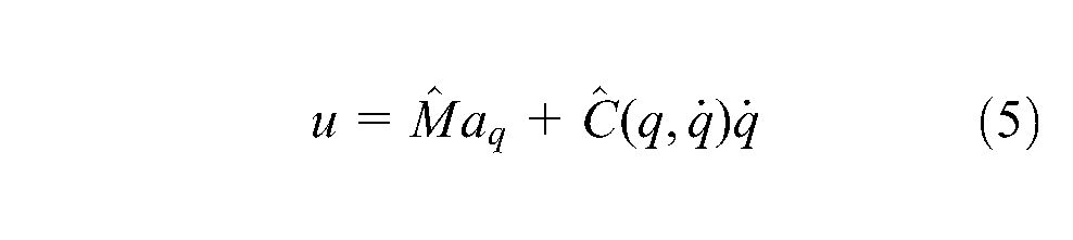
where
Substituting Equation (5) into Equation (1) we obtain
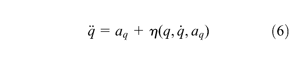
where
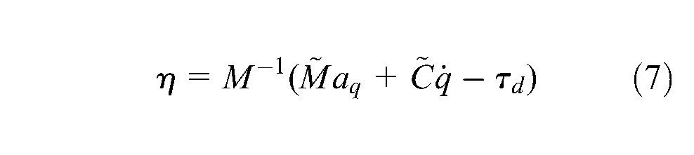
It can be noted from Equation (6) that the system is still non-linear and coupled due to the uncertainty
From Equation (6), the error equation can be obtained as
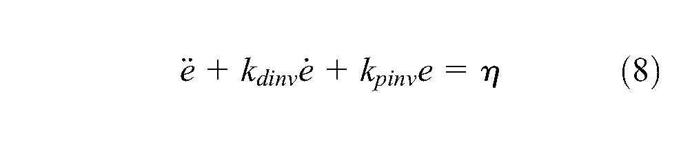
The right side of the error equation above is not equal to zero, and so the convergence of the tracking errors is no longer guaranteed by the inverse dynamics-based controller given in Equation(5); thus the desired tracking performance specifications are not satisfied. Therefore, in order to improve the robustness and to reduce the coupling, it requires compensation for the uncertainties by controller.
Large servo errors caused by low-frequency disturbances and high-frequency noise
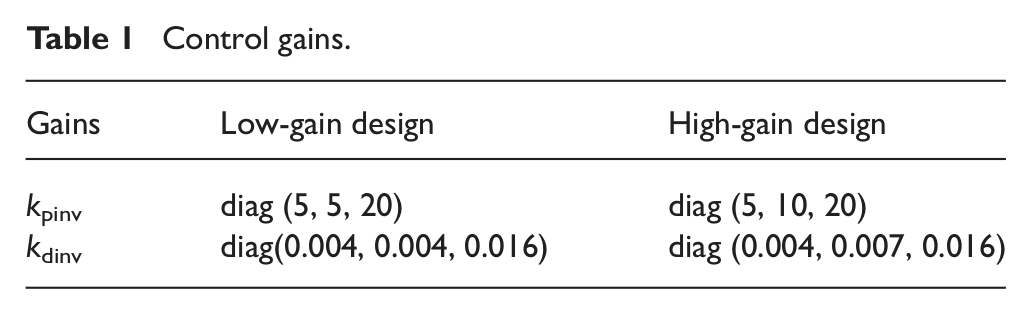
Another example for the requirement of the proposed non-linear controller is shown as follows. A linear inverse dynamics controller with low gain and that with high gain are used, respectively. The gain kdinv in the Equation (5) is changed together with the gain kpinv in order to ensure the stability of the controller. The control parameters are shown in Table 1. These parameters are chosen by a number of experiments, in which these parameters show relatively better performance. The motion is in the Y-direction, so only the comparison of the gains kpinv and kdinv related to this motion are conducted. Closed-loop performance is assessed on the centre position of the motor. At this location, a motion in the Y-direction is conducted using the trajectory shown in Figure 7. The maximum acceleration is 10 m/s2, the maximum speed is 0.25 m/s and the stroke is 0.1 m.
Control gains.
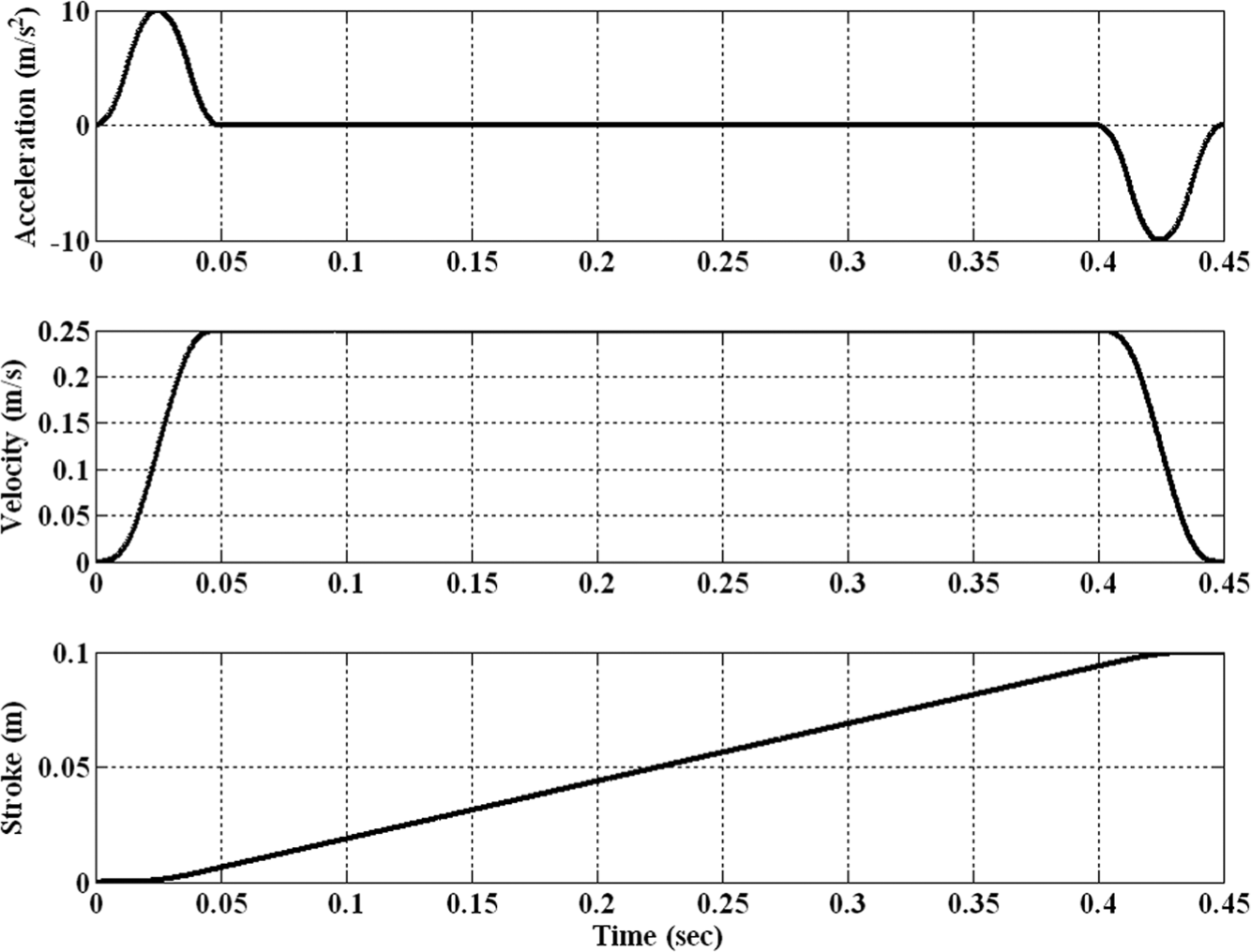
Tracking trajectory in experiment 1.
Figure 8 shows the tracking errors in the Y-direction. Figures 9 and 10 are time–frequency analyses of the tracking error signal. More specifically, they show contour plots of the energy of the measured signal in the time–frequency plane. Herein, the colour bar shows a linear scale from the smallest amplitude encountered (blue) toward the largest amplitude encountered (red). A detailed study of Figure 9 shows that the servo error characteristics during moving possess one dominant low-frequency (50 Hz) oscillation with an amplitude level of 1 µm, which can be benefit from an increased controller gain. With a linear high-gain controller, the result in terms of time–frequency analysis is considered in Figure 10. Herein the dominant low-frequency contributions are almost completely removed from the error responses compared with the linear low-gain design. However, the maximum tracking errors during uniform motion are 1 µm, which are not the desired servo performance. This is because an increased controller gain potentially deteriorates the servo performance by inducing the amplification of high-frequency noise. To derive a solution to the problem highlighted in the linear feedback, an amplitude-based variable-gain control design will be developed.
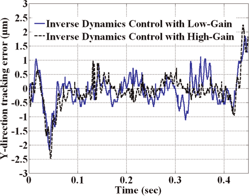
Y-direction tracking error of linear inversed dynamics control law.
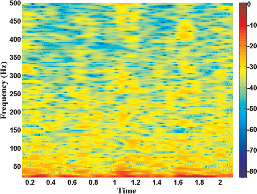
Time–frequency analysis of the errors of inversed dynamics control law with low gain.
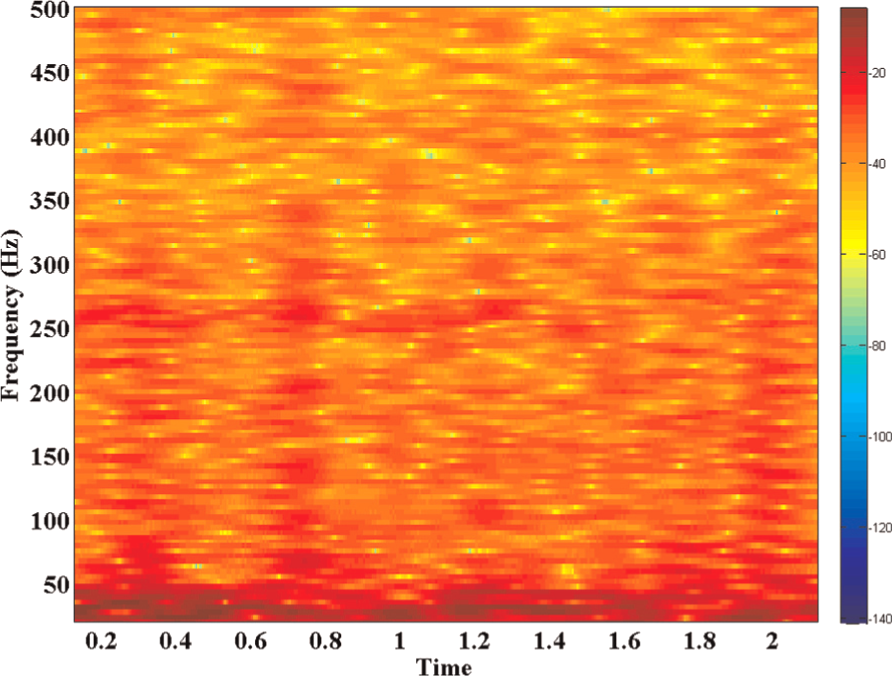
Time–frequency analysis of the errors of inversed dynamics control law with high gain.
Non-linear composite control algorithm
In order to improve the stability and the servo performance, a non-linear controller is proposed for planar motor with dynamic uncertainties. The control schematic diagram of the 3-DOF planar motor is shown in Figure 11.
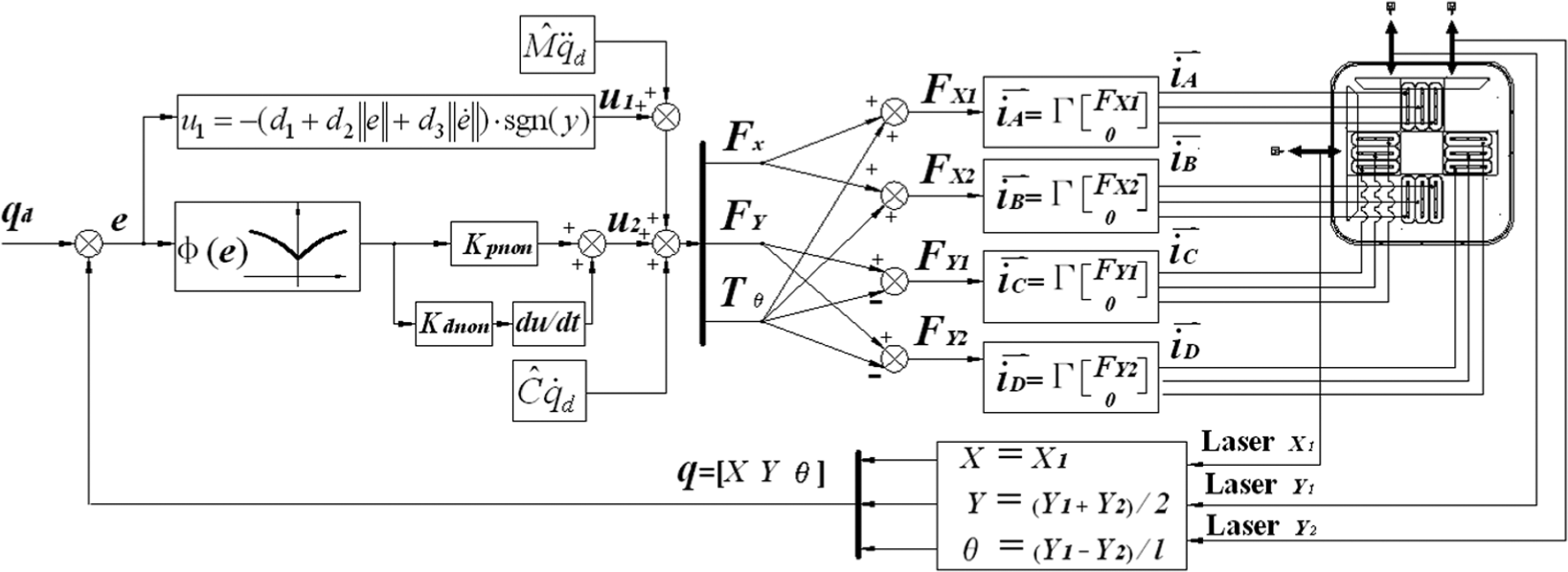
Control schematic diagram.
The proposed control law combines u1 and u2 terms, such that

where u is the control input,
Introducing a variable y(e) as
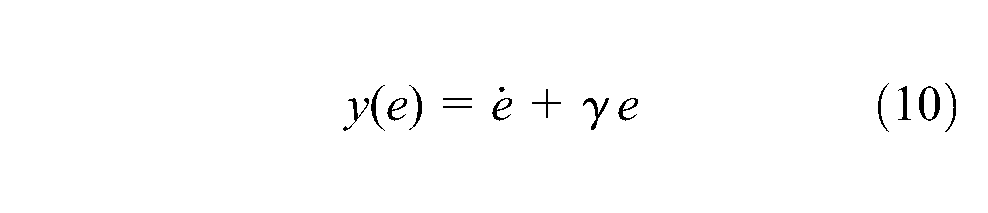
where
Then the robust term u1 is given by
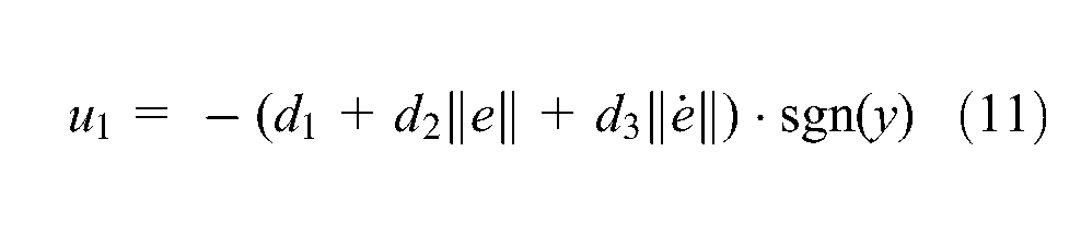
where d1, d2 and d3 are positive constants.
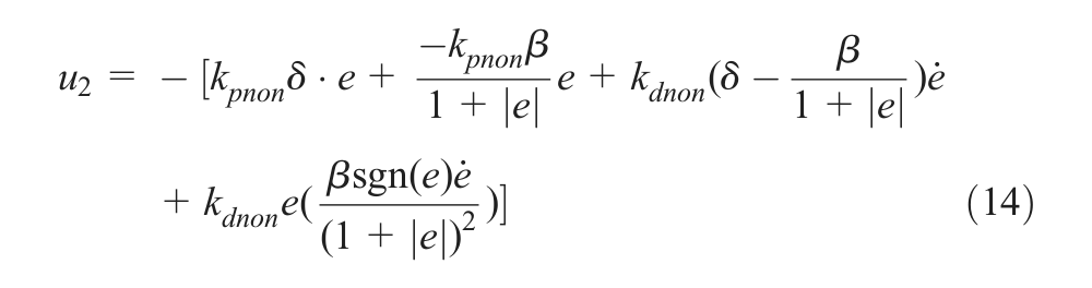
The term u2 is give by
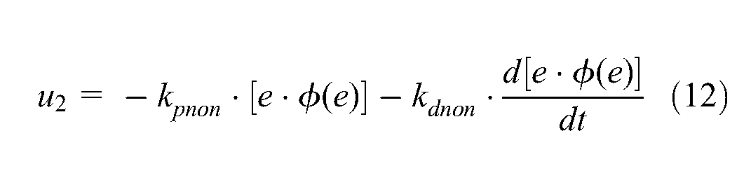
where k pnon and k dnon are control gains.
For the purpose of variable-gain control, a non-linear function is applied
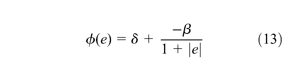
where
The variable-gain characteristics along with the static input–output non-linearity, described by Equation (13), are shown in Figure 12.
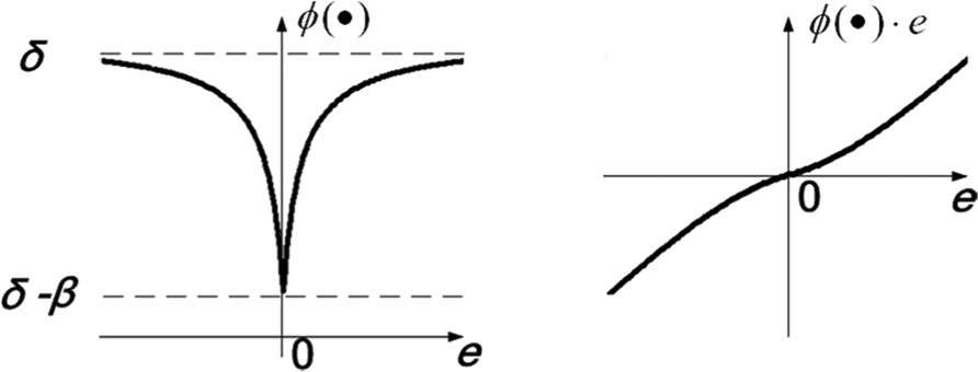
Variable-gain characteristics.
From Equations (12) and (13),
Subtracting
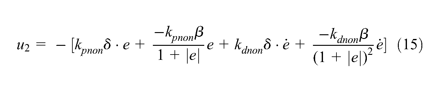
Therefore, the control term u2 can be rewritten as
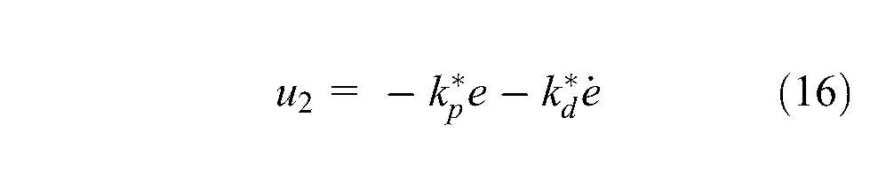
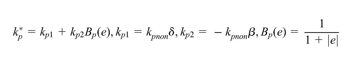
where

See the Appendix for the stability analysis, which is based on the Lyapunov stability theory.
Experiments
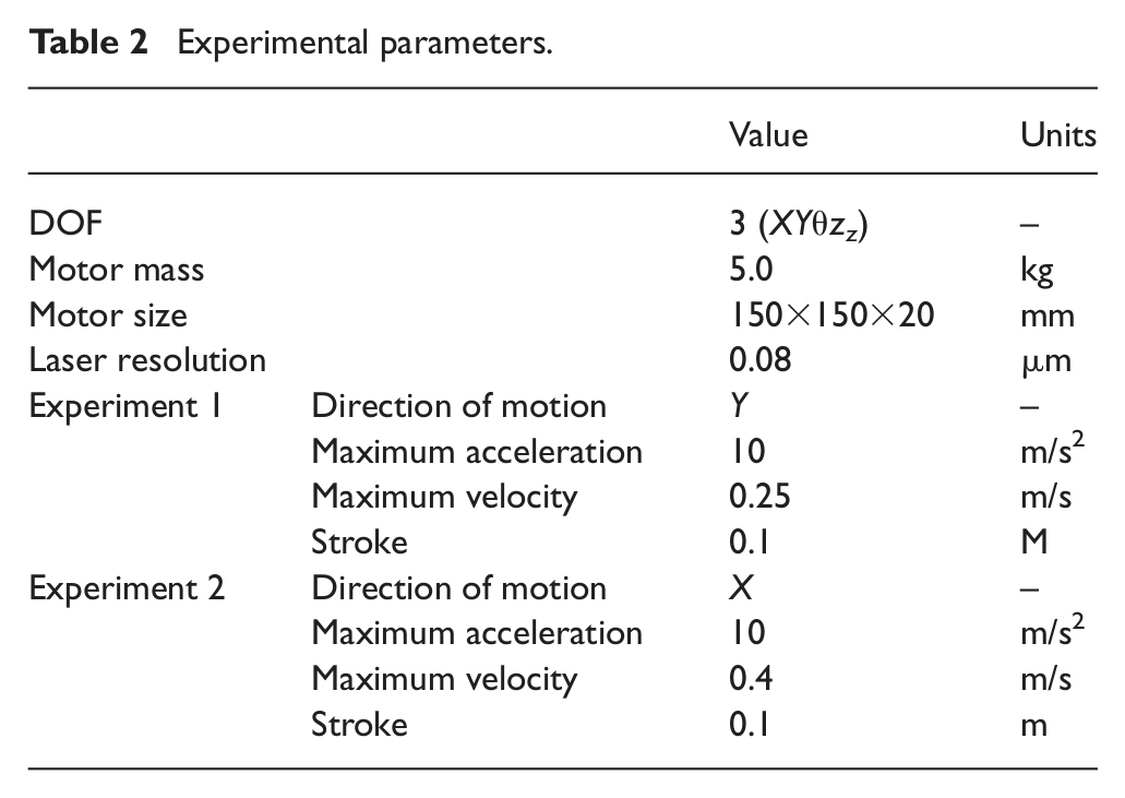
Both the inverse dynamics controllers and the non-linear controller are carried out to verify the effectiveness of the control law proposed in this paper, the parameters of which are listed in Table 2. The corresponding trajectories tracked in the two experiments are shown in Figures 7 and 13, respectively, with the desired rotational motion angle equal to zero.
Experimental parameters.
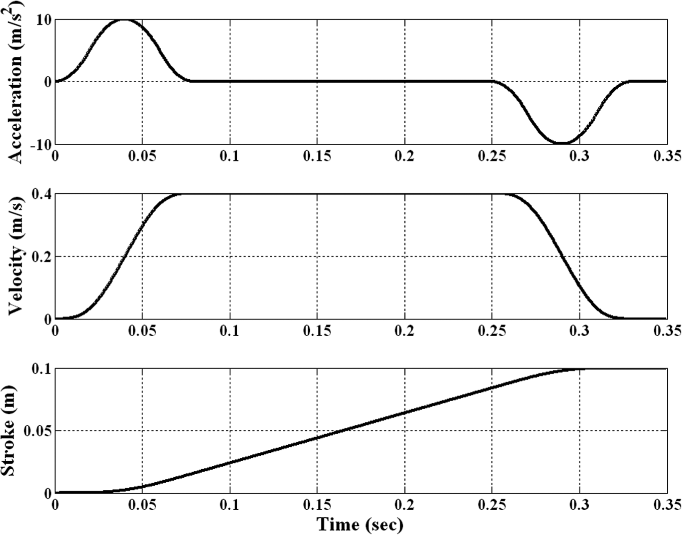
Tracking trajectory in experiment 2.
The servo control system is discrete in practical applications; the discrete expression of the controller is given as follows, where the sampling frequency is 5000 Hz.
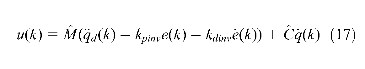
The discrete expression of the controller in Equation (5) is
The discrete expression of the controller in Equation (9) is
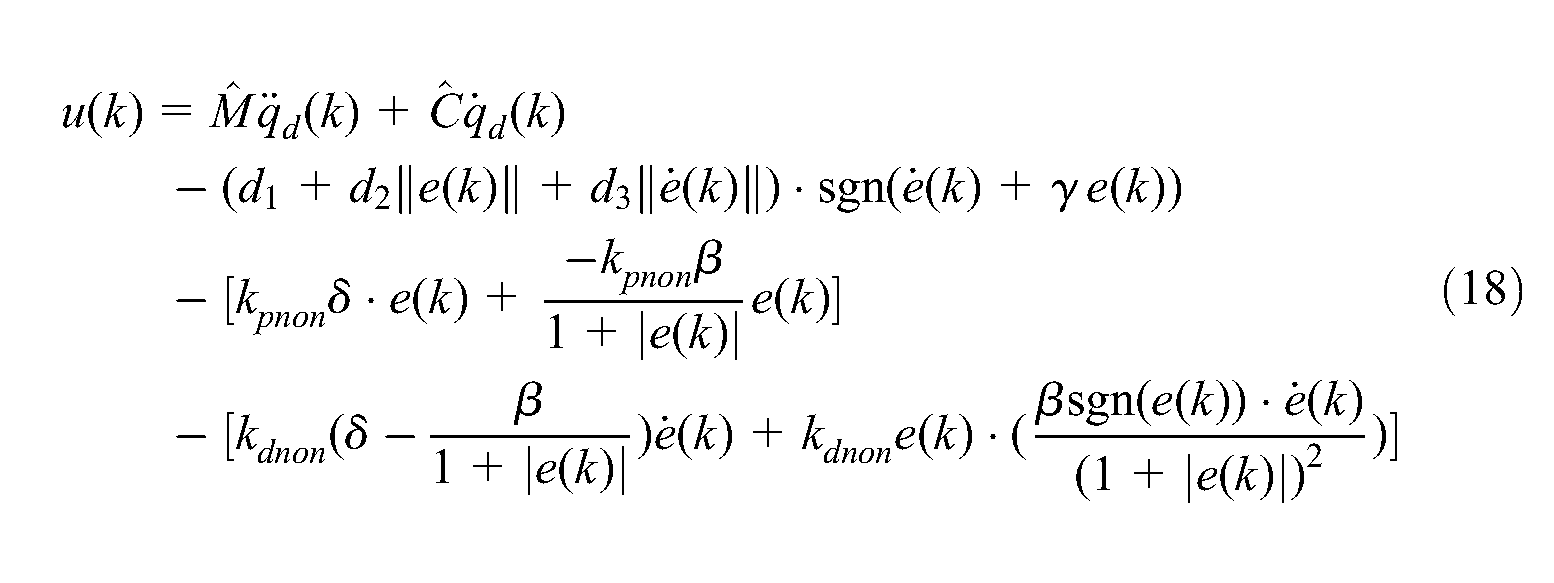
where
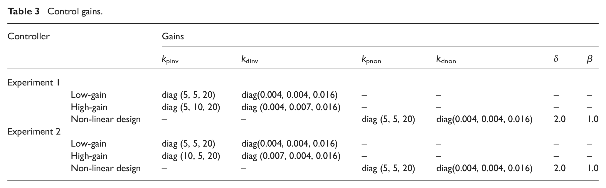
The control parameters are shown in Table 3. These parameters are chosen by a number of experiments, in which these parameters show a relatively better performance.
Control gains.
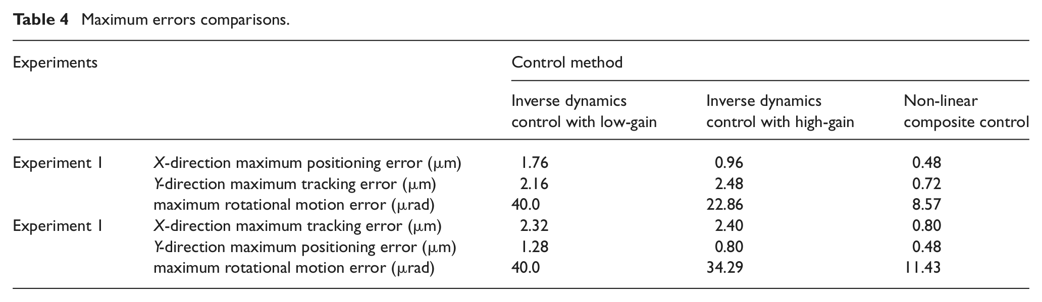
The results of experiment 1 are shown in Figures 14–17; those of experiment 2 are shown in Figures 18–23. The maximum errors are listed in Table 4.
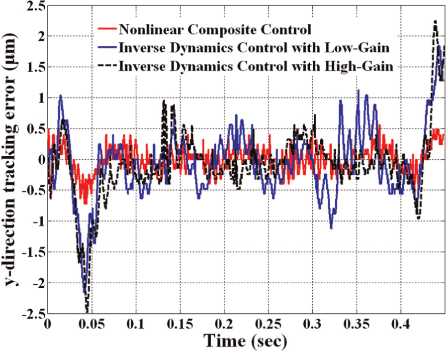
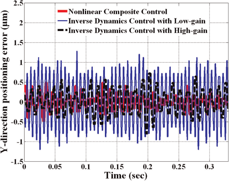
Y-direction tracking error comparison in experiment 1.

Time–frequency analysis of the errors of non-linear composite control law in experiment 1.
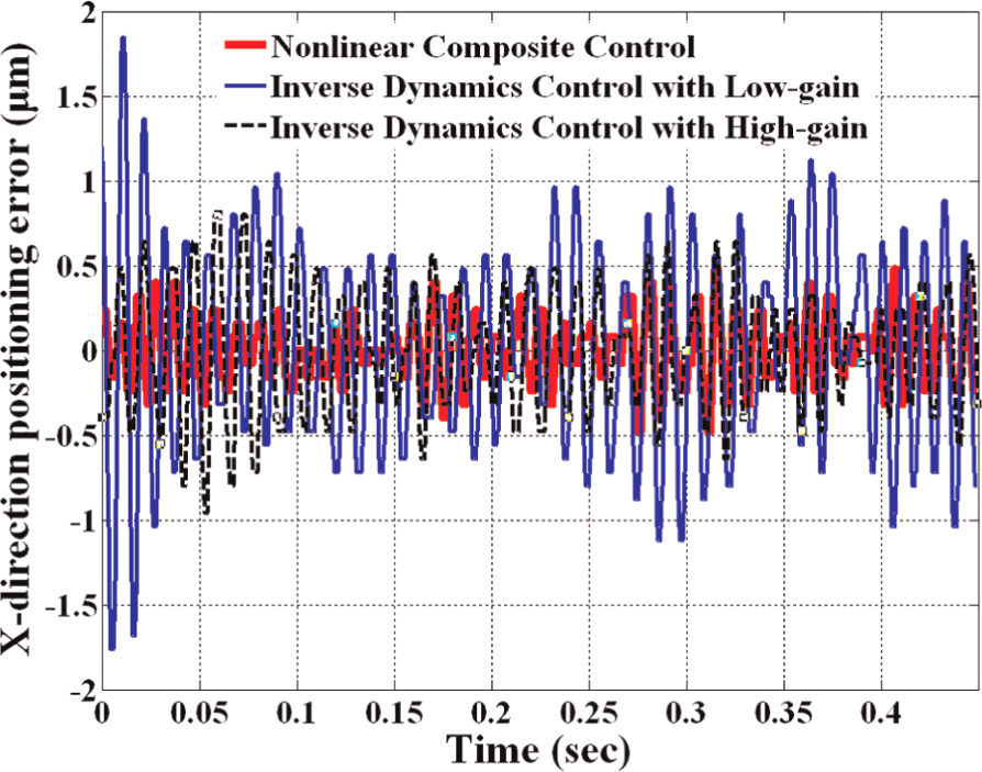
X-direction positioning error comparison in experiment 1.
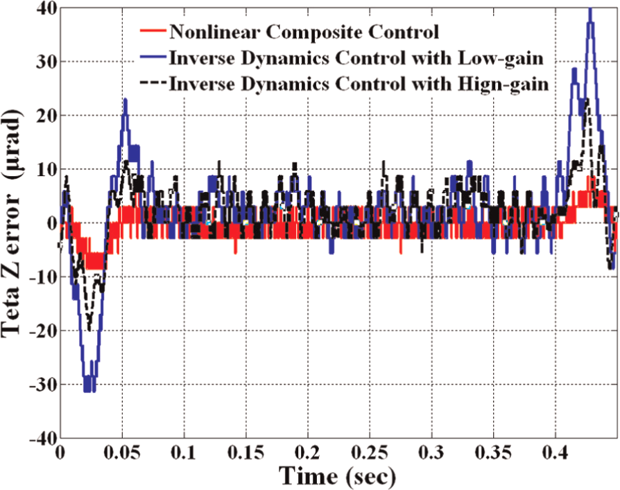
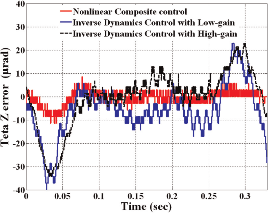
θz positioning error comparison in experiment 1.
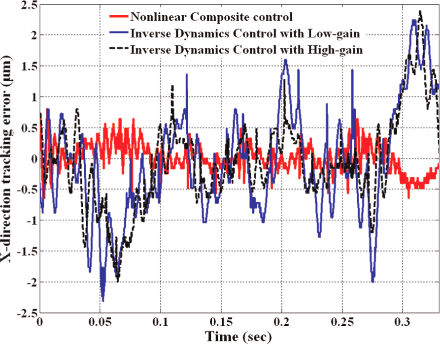
X-direction tracking error comparison in experiment 2.
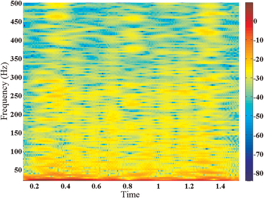
Time–frequency analysis of the errors of inversed dynamics control with low gain in experiment 2.
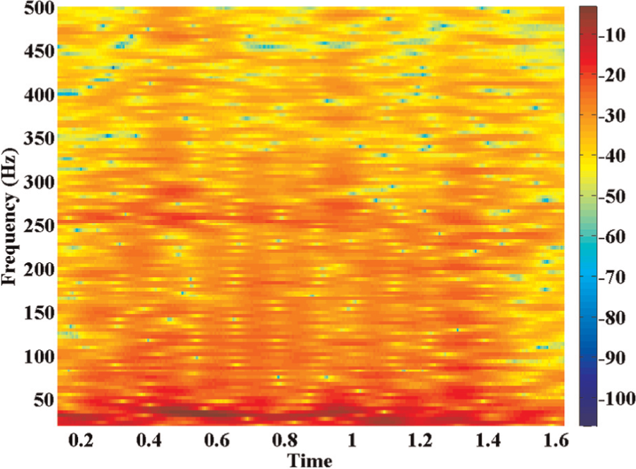
Time–frequency analysis of the errors of inversed dynamics control with high gain in experiment 2.
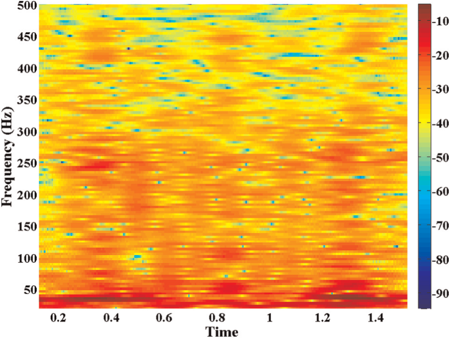
Time–frequency analysis of the errors of non-linear composite control law in experiment 2.
Y-direction positioning error comparison in experiment 2.
θz positioning error comparison in experiment 2.
Maximum errors comparisons.
It can be seen from the experimental results that the maximum tracking error and the maximum rotational motion error occur at about the same time as the peak acceleration or deceleration, and this demonstrates that due to the modelling errors, there exists some coupling between the multi-degrees of freedom and that this MIMO system cannot be decoupled. It is also shown that, compensating for the modelling errors using u1 in the non-linear composite control law, the effects of the coupling between multi-degrees of freedom are reduced, and therefore the positioning precision is improved.
It is clearly observed from the results above that by comparing the results of the time–frequency analysis in Figures 9 and 19, the closed-loop resonance frequency achieved by linear low-gain controller is about 50 Hz. This frequency is located sufficiently below the controller bandwidth that the low-frequency disturbance limits the system performance. The linear high-gain controller seems capable of removing the low-frequency contributions, seen from Figures 10 and 20, but the tracking performance and the positioning ability are also not good. This is because the high-frequency contents are then amplified under high-gain feedback, and as a result, a deteriorated performance ensues. Compared with both linear controllers, the amplitude-based variable-gain controller appears to show good performance in its ability to suppress the low-frequency behaviour equally as well as the linear high-gain design. In terms of dominant high frequencies, however, the amplitude-based non-linear design shows less dominant behaviour of the closed-loop resonance frequency in the servo error responses, thereby limiting the amplification of noise. Due to the ability continuously to balance the trade-off between disturbance rejection and measurement noise sensitivity, the tracking errors are smaller than the results using both the linear controllers. Thus the tracking performance and the robustness of the system are greatly improved by the non-linear composite controller.
The experiments above are linear motion, and in order to show fully the servo performance of the non-linear controller, the trajectory tracking performance is assessed and compared based on a planar motion experiment, in which additional coupling effects, as centrifugal and Coriolis forces can be reflected.
The planar circular motion equation is
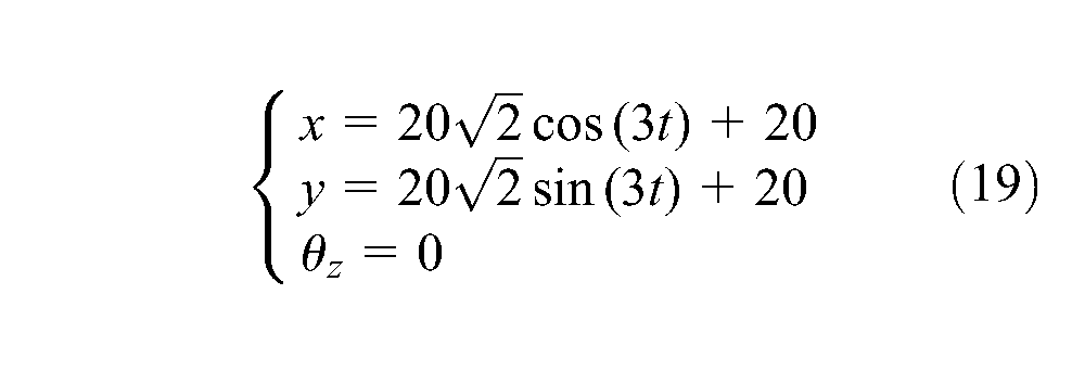
The unit of the above equation is millimetres. The tracking trajectory is shown in Figure 24.
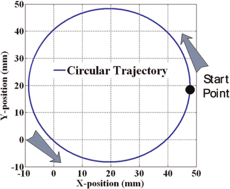
Circular motion trajectory.
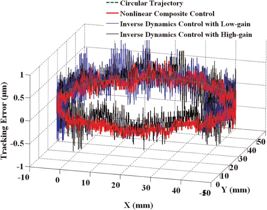
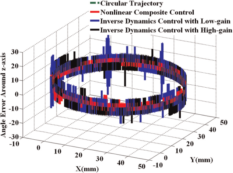
Define the tracking error as
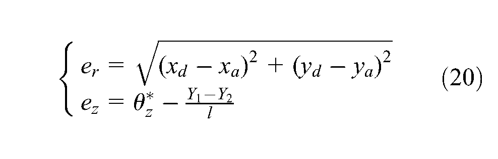
where e
r
is the radial error, ez is the rotational motion error around the z-axis,
Figures 25 and 26 show the tracking errors during the circular motion. The maximum tracking errors are listed in Table 5.
Tracking radial errors during circular motion.
Rotational motion errors around z-axis during circular motion.
The maximum tracking errors during circular motion.
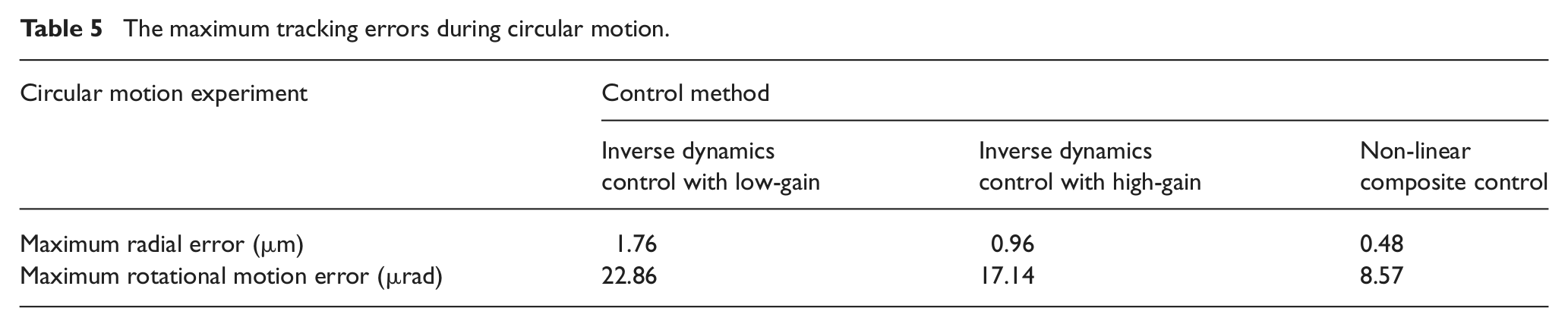
These results show that the non-linear controller effectively reduces the coupling between the multi-DOFs and has the potential to improve upon servo performance significantly. It is an attractive control approach for the uncertain multi-DOF systems.
Conclusion
A 3-DOF planar motor, which is composed of four air bearings, four linear motors and a three-axis laser, is discussed in this paper. A decoupled dynamic model is established. The detailed presentation of the non-linear composite controller design and performance evaluation in practice is given.
To verify the effectiveness of the developed controller, two linear motions along the Y- and X-directions and planar motion are carried out, respectively. It is clearly observed from the experimental results that the interference between the XYθz drive axes is reduced by compensating for the modelling errors.
Moreover, from time–frequency analysis on the servo error, both two linear controllers, a low-gain as well as a high-gain controller, are bounded to the fixed trade-off between the disturbance suppression and measurement noise sensitivity. The linear inverse dynamics control under low gain limits the amplification of noise, with less favourable disturbance rejection properties, whereas the linear inverse dynamics control under a high-gain design shows improved disturbance rejection at the cost of high-frequency noise amplification. Conversely, non-linear control, or more specifically amplitude-based variable-gain control, is considered a means to deal with this fixed trade-off. Compared with both linear design limits, the amplitude-based variable gain is able to balance continuously the improved disturbance rejection with desirable noise sensitivity, and therefore the tracking and the positioning errors are smaller than the results obtained by the linear controller.
Footnotes
Appendix: The stability analysis of the non-linear composite control law
According the variable y(e), the dynamics of the planar can be rewritten as
Define the Lyapunov function as
Time differentiation of Equation (A2) gives
According to Equations (9), (16) and (A1), this gives
where w includes the modelling errors and
Without loss of generality, assume w is bounded as
Subtracting Equations (A4) and (A5) into Equation (A3) gives
According to the variable y(e), the following are obtained
Subtracting Equation (A8) to Equation (A7) gives
The planar motor is 3-DOF, therefore
Subtracting Equations (A10) and (A11) into Equation (A9) gives
Since
Therefore
Subtracting Equation (A14) to Equation (A12) gives
Since the inequalities of
If the control gains satisfy the following inequalities
then
Since
therefore
and the condition for Lyapunov stability is satisfied.
Acknowledgements
This work is supported by the National Basic Research Program of China 973 Program (2009CB724205).
Funding
This research received no specific grant from any funding agency in the public, commercial, or not-for-profit sectors.