Reinforcement learning-based intelligent tracking control for wheeled mobile robot

Abstract

This paper proposes a new method to design a reinforcement learning-based integrated kinematic and dynamic tracking control algorithm for a non-holonomic wheeled mobile robot without knowledge of the system’s drift tracking dynamics. The actor critic structure in the control scheme uses only one neural network to reduce computational cost and storage resources. A novel tuning law for a single neural network is designed to learn an online solution of a tracking Hamilton–Jacobi–Isaacs (HJI) equation. The HJI solution is used to approximate an H_∞ optimal tracking performance index function and an intelligent tracking control law in the case of the worst disturbance. The laws guarantee closed-loop stability in real time. The convergence and stability of the overall system are proved by Lyapunov techniques. The simulation results on a non-linear system and wheeled mobile robot verify the effectiveness of the proposed controller.

Keywords

Actor critic Hamilton–Jacobi–Isaacs equation neural network wheeled mobile robot

Introduction

An important motion control problem for the system of wheeled mobile robots (WMRs) is the trajectory tracking. This problem has been extensively studied in past few decades. Generally, a variety of control algorithms for the trajectory tracking problem has been devoted in the form of adaptive control (Fierro and Lewis, 1998; Marvin et al., 2009; Mohareri et al., 2012) where the back-stepping techniques are used. The kinematic controllers are designed using the available models, and dynamic controllers are designed based on neural networks (NNs). They are considered indirect adaptive controllers. Besides, they do not minimize any long-term performance function and hence are not optimal. H_∞ adaptive control for a WMR based on inverse optimality is proposed in Miyasato (2008) but it is an offline control scheme. A specific characteristic of the WMR models is that it can be presented as a non-linear system in a strict-feedback form, but until now, to the best knowledge of the authors, methods of tracking control for a WMR using this form are just considered in adaptive back-stepping (Chwa, 2010) or adaptive feedback linearization schemes (Khoshnam et al., 2011) without any optimality.

In the other direction, thanks to the abilities of online adaptive learning of reinforcement learning (RL) methods in optimal control, tracking control methods for WMRs have been studied. The adaptive critic structures in RL are exploited to learn discrete controllers (Lin and Yang, 2008; Zenon and Marcin, 2011) or a continuous controller without disturbance using the learned solution of the Hamilton–Jacobi–Bellman (HJB) equation (Luy, 2012). These controllers not only overcome the drawbacks of the other methods such as the domain expert of fuzzy or existing controllers to generate a training sample for NNs, but also optimize utility functions, in contrast to the tracking error at the current time instant in the NN-based adaptive controllers. However, these methods have access to the known explicit model of WMR and ignored the disturbance, so they are not a type of robust adaptive control method.

To control a non-linear system, i.e. a WMR system with optimality related to disturbances using RL, the solutions of Hamilton–Jacobi–Isaacs (HJI) in the $H_{\infty}$ optimal control problem must be learned (Dierks and Jagannathan, 2010). The integral RL-based direct adaptive control algorithm for a class of general non-linear system has been studied in Vamvoudakis et al. (2011) to solve the HJI equation. The most favourable part of this algorithm is that NNs can be trained synchronously to approximate optimal control input and worst-case disturbance without knowledge of the system drift dynamics terms. However, it requires three NNs in the same structure – one for the critic and the others for actors. The number of neurons in the hidden layers should be at least (n+1)n/2, where n is number of state variables. In practical applications, e.g. robotics, the number of state variables measured from sensors for feedback may be relatively large. With three NNs, the number of NNs weights and the activation functions representing the elements in combination of the states will significantly increase. If applied directly, the algorithm to a non-linear system may lead to the computational complexity and resource consumption. In contrast, a method using a single online approximator (SOLA) in Dierks and Jagannathan (2010) to solve the HJI equation can reduce the number of NNs but, unfortunately, it is a type of model-based RL.

From the aforementioned problems, there are three main contributions in the paper. The first involves the derivation of a tracking dynamics formed from a non-linear strict-feedback model of WMR the purpose of which is to design an integrated kinematic and dynamic control RL based-intelligent controller, i.e. the integrated kinematic and dynamic robust direct adaptive tracking controller with optimality without explicit knowledge of the system’s drift dynamics. The actor critic structure in the RL scheme uses only one NN for the critic law. Secondly, the last contribution is the tuning law for the critic NN so that solutions of the tracking HJI equation are learned, and optimality values of the tracking performance index function and the robust direct adaptive control law as well as the worst-case disturbance law are approximated without accessing the system’s drift dynamics. By Lyapunov techniques, the closed-loop system state and critic NN error are proved to be uniform ultimate bounds and system parameters show convergence to optimal target values asymptotically.

The paper is organized as follows. The next section provides the theoretical background of the WMR to establish the non-linear WMR system in the strict-feedback form and then the new tracking dynamics is derived. Then we design the integrated kinematic and dynamic robust direct adaptive tracking control scheme with optimality along with tuning law for the critic NN and give proof of stability and convergence. The results of simulation on the WMR verify the effectiveness of the proposed algorithm and conclusions are drawn.

Strict-feedback kinematic and dynamic model

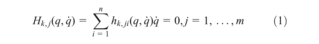
A WMR with differentially driven wheels mounted on a driving axle can move and rotate on the horizontal plane thanks to two independent actuators. Torque from the actuators is transmitted to the left and the right wheels to drive the robot. The mass of the WMR including the mass of the platform without the wheels and the mass of the wheels is focused on a central point. The distance of the driven wheels is b₁. The radius of each wheel is r₁. The distance from the centre point to the driving axe is l. Without loss of generality, it can be assume that l=0. The WMR is considered a mechanical system with n generalized configuration variables q suffering m constraints (m<n) and represented by the equation as follows (Khoshnam et al., 2011)

H_{k, j} (q, \overset{\cdot}{q}) = \sum_{i = 1}^{n} h_{k, ji} (q, \overset{\cdot}{q}) \overset{\cdot}{q} = 0, j = 1, \dots, m

(1)

where the number of holonomic and non-holonomic constrains are k and m−k, respectively. The constrains are independent of time and can be written as $A_{k} (q) \overset{\cdot}{q} = 0$ , where $A_{k} \in ℜ^{m \times n}$ is a full-rank matrix. Assume that $S (q) \in ℜ^{n \times (n - m)}$ is also a full-rank matrix that is formed from a set of smooth and linearly independent vector fields in the null space of $A_{k}$ such that $A_{k} (q) S (q) = 0$ . Let $ϑ (t) \in ℜ^{n - m}$ be the velocity vector, which can be seen as the pseudo-control vector, and is important to form a strict-feedback non-linear system afterwards. The kinematic equation of WMR motion can be written as

\overset{\cdot}{q} = S (q) ϑ (t)

(2)

To derive a dynamic equation of WMR, Lagrange formalism is used as follows

\frac{d}{dt} (\frac{\partial L}{\partial \overset{\cdot}{q}}) - \frac{\partial L}{\partial \overset{\cdot}{q}} = F_{T}

(3)

where $F_{T}$ is the vector of the generalized forces. The WMR moves on a plane so Lagrangian L only includes kinetic energy

L = \frac{1}{2} \sum_{i = 1}^{n_{i}} v_{i}^{T} m_{i} v_{i} + ω_{i}^{T} I_{i} ω_{i}

(4)

where $v_{i}$ , $ω_{i}$ , $m_{i}$ and $I_{i}$ are elements of the linear velocity, the rotation velocity, the mass and the moment of inertia, respectively. As a result, the dynamic model of the WMR is expressed as

M (q) \overset{\cdot\cdot}{q} + C (q, \overset{\cdot}{q}) \overset{\cdot}{q} + B (q) F (\overset{\cdot}{q}) + B (q) τ_{d} = B (q) τ - A_{k}^{T} (q) λ

(5)

where $M (q) \in ℜ^{n \times n}$ is the symmetric positive defined inertia matrix, $C (q, \overset{\cdot}{q}) \in ℜ^{n \times n}$ is the centripetal and Coriolis matrix, $F (\overset{\cdot}{q}) \in ℜ^{n \times 1}$ is the surface friction and gravitational vector, $τ_{d} \in ℜ^{(n - m) \times 1}$ denotes the bounded unknown disturbances including unstructured unmodelled dynamics, $B (q) \in ℜ^{n \times (n - m)}$ is the input transformation matrix, $τ \in ℜ^{(n - m) \times 1}$ is the input torque vector and $λ \in ℜ^{m \times 1}$ is the vector of constraint forces. Taking the time derivative of the kinematic model (2), one obtains

\overset{\cdot\cdot}{q} = \overset{\cdot}{S} (q) ϑ + S (q) \overset{\cdot}{ϑ}

(6)

Substituting (2), (6) into (5) and multiplying both sides of the result by $S^{T} (q)$ and note that $A_{k} (\overset{\cdot}{q}) S (q) = 0$ , one obtains

\bar{M} (q) \overset{\cdot}{ϑ} (t) + \bar{C} (q, \overset{\cdot}{q}) ϑ (t) + \bar{F} (\overset{\cdot}{q}) + {\bar{τ}}_{d} = \bar{B} (q) τ

(7)

where $\bar{M} (q) = S^{T} MS$ , $\bar{C} (q, \overset{\cdot}{q}) = S^{T} MS + S^{T} CS$ , $\bar{B} (q) = S^{T} B$ , $\bar{F} (\overset{\cdot}{q}) = S^{T} M \overset{\cdot}{S} ϑ + \bar{B} F$ , ${\bar{τ}}_{d} = \bar{B} τ_{d}$ .

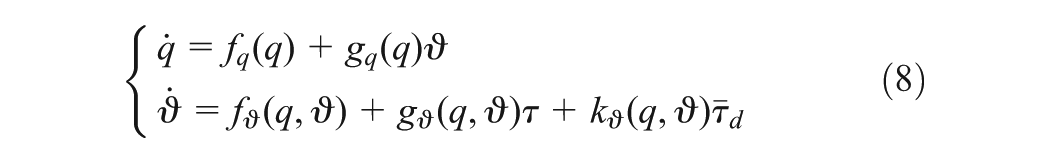
Definition 1. Letting $f_{q} (q) = 0_{n \times 1}$ , $g_{q} (q) = S (q) \in ℜ^{n \times (n - m)}$ , $f_{ϑ} (q, ϑ) = - {\bar{M}}^{- 1} (q) (\bar{C} (\overset{\cdot}{q}, q) ϑ + \bar{F} (\overset{\cdot}{q})) \in ℜ^{(n - m) \times 1}$ , $g_{ϑ} (q, ϑ) = {\bar{M}}^{- 1} (q) \bar{B} (q) \in ℜ^{(n - m) \times (n - m)}$ , $k_{ϑ} (q, ϑ) = {\bar{M}}^{- 1} (q) \in ℜ^{(n - m) \times (n - m)}$ .

The state space equation of WMR represented the non-linear system in the strict-feedback form is obtained by using kinematics and dynamics Equations (2) and (7)

{\begin{matrix} \overset{\cdot}{q} = f_{q} (q) + g_{q} (q) ϑ \\ \overset{\cdot}{ϑ} = f_{ϑ} (q, ϑ) + g_{ϑ} (q, ϑ) τ + k_{ϑ} (q, ϑ) {\bar{τ}}_{d} \end{matrix}

(8)

The system (8) is assumed to be controllable and drift free with $(q, ϑ) = 0$ , a unique equilibrium point on a compact set $X \in ℜ^{2 n - m}$ . Let us view some following important properties.

Property 1. $\bar{M} (q)$ is a bounded asymmetric and positive definite matrix such that ${\bar{m}}_{min} \leq ‖ \bar{M} (q) ‖ \leq {\bar{m}}_{max}$ , where ${\bar{m}}_{min}$ and ${\bar{m}}_{max}$ are positive scalar constants.

Property 2. $\bar{C} (q)$ is bounded such that $c_{min} \leq ‖ \bar{C} (q) ‖ \leq c_{max}$ , where $c_{min}$ and $c_{max}$ are positive scalar constants.

Property 3. The disturbance ${\bar{τ}}_{d}$ is bounded such that $‖ {\bar{τ}}_{d} ‖ \leq τ_{d max}$ , where $τ_{d max}$ is a positive scalar constant.

Property 4. $f_{ϑ} (q, ϑ)$ is the system uncertainty dynamics term and $f_{ϑ} (q, ϑ) \leq - c_{max} {\bar{m}}_{min}^{- 1} ‖ ϑ ‖$ .

Property 5. $g_{q} (q)$ is bounded such that $g_{min} \leq ‖ g_{q} (q) ‖ \leq g_{max}$ , where $g_{min}$ and $g_{max}$ are positive scalar constants.

Property 6. $g_{ϑ} (q, ϑ)$ is bounded such that ${\bar{m}}_{max}^{- 1} \bar{B} \leq ‖ g_{ϑ} (q, ϑ) ‖ \leq {\bar{m}}_{min}^{- 1} \bar{B}$ , where $\bar{B} (q)$ , the constant non-singular matrix, depends on the geometric parameter of the WMR, i.e. the radius $r_{1}$ of wheels and the robot frame width $b_{1}$ (Khoshnam et al., 2011), and according to Property 1, $g_{ϑ} (q, ϑ) \neq 0$ .

Property 7. $k_{ϑ} (q, ϑ)$ is bounded such that ${\bar{m}}_{max}^{- 1} \leq ‖ k_{ϑ} (q, ϑ) ‖ \leq {\bar{m}}_{min}^{- 1}$ and according to Property 1 $k_{ϑ} (q, ϑ) \neq 0$ .

Property 8. $f_{ϑ} (q, ϑ)$ , $g_{q} (q)$ , $g_{ϑ} (q, ϑ)$ and $k_{ϑ} (q, ϑ)$ are non-linear smooth functions.

Definition 2. If a reference robot generates the bounded smooth trajectory vector that satisfies the constraint ${\overset{\cdot}{q}}_{d} = S (q_{d}) ϑ_{rd}$ , where $ϑ_{rd}$ is the smooth velocity vector, the main objective for the robust adaptive tracking control problem for WMR is to design integrated kinematic and dynamic feedback control laws for the dynamic system (8) where contains the uncertainty terms and disturbance, such that when $t \to 0$ , then $e_{q} \to 0$ with $e_{q} = q - q_{d}$ . Furthermore, a defined tracking cost function related to (8) must be optimized.

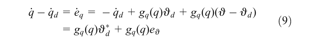
To have tracking dynamics for designing integrated kinematic and dynamic feedback control law, some steps to change model (8) will be executed. The first equation in (8) is written as

\begin{matrix} \overset{\cdot}{q} - {\overset{\cdot}{q}}_{d} = {\overset{\cdot}{e}}_{q} = - {\overset{\cdot}{q}}_{d} + g_{q} (q) ϑ_{d} + g_{q} (q) (ϑ - ϑ_{d}) \\ = g_{q} (q) ϑ_{d}^{*} + g_{q} (q) e_{ϑ} \end{matrix}

(9)

where $e_{ϑ} = ϑ - ϑ_{d} \in ℜ^{n - m}$ , $ϑ_{d} \in ℜ^{n - m}$ is virtual control input such that $ϑ_{d} = ϑ_{d}^{*} + ϑ_{da}$ with $ϑ_{d}^{*} \in ℜ^{n - m}$ is an optimal tracking control input vector designed later, and $ϑ_{da}$ , the feed-forward virtual control input, is the solution of the equation

0 = - {\overset{\cdot}{q}}_{d} + g_{q} (q) ϑ_{da}

(10)

Similarly, the last equation in (8) is written as

\begin{matrix} \overset{\cdot}{ϑ} - {\overset{\cdot}{ϑ}}_{d} = {\overset{\cdot}{e}}_{ϑ} = - {\overset{\cdot}{ϑ}}_{d} + f_{ϑ} (q, ϑ) + g_{ϑ} (q, ϑ) τ + k_{ϑ} (q, ϑ) {\bar{τ}}_{d} \\ = f_{ϑ} (q, ϑ) + g_{ϑ} (q, ϑ) τ^{*} - g_{q}^{T} (q) e_{q} + k_{ϑ} (q, ϑ) {\bar{τ}}_{d} \end{matrix}

(11)

where $τ^{*}$ is the tracking control input designed later such that $τ = τ^{*} + τ_{a}$ and $τ_{a}$ is a solution of the equation

0 = - {\overset{\cdot}{ϑ}}_{d} + g_{ϑ} (q, ϑ) τ_{a} + g_{q}^{T} (q) e_{q}

(12)

Definition 3. Let $x_{d} = {[q_{d}^{T}, ϑ_{d}^{T}]}^{T} \in ℜ^{(2 n - m) \times 1}$ , $x = {[q^{T}, ϑ^{T}]}^{T} \in ℜ^{(2 n - m) \times 1}$ , $e = {[e_{q}^{T}, e_{ϑ}^{T}]}^{T} \in ℜ^{2 n - m}$ , $f (x) = {[0_{n \times 1}, f_{ϑ}^{T} (q, ϑ)]}^{T} \in ℜ^{2 n - m}$ , $u^{*} = u - u_{a}$ , $u^{*} = {[ϑ_{d}^{* T}, τ^{* T}]}^{T} \in ℜ^{2 (n - m) \times 1}$ , $u_{a} = {[ϑ_{da}^{T}, τ_{a}^{T}]}^{T} \in ℜ^{2 (n - m) \times 1}$ , $g (x) = diag [g_{q} (q), g_{ϑ} (x)] \in ℜ^{(2 n - m) \times 2 (n - m)}$ , $k (x) = diag [k_{q} (q), k_{ϑ} (q, ϑ)] \in ℜ^{(2 n - m) \times 2 (n - m)}$ , $k_{q} (q) = 0_{n \times (n - m)}$ , $d = {[0_{1 \times (n - m)}, {\bar{τ}}_{d}^{T}]}^{T} \in ℜ^{2 (n - m) \times 1}$ .

Lemma 1. Consider the tracking dynamics of the WMR as follows

\overset{\cdot}{e} = f (x) + g (x) u^{*} + k (x) d

(13)

If the control law $u^{*}$ for (13) is designed, it can be the control law for (8), that means the control law $u^{*}$ for (13) and (8) is equivalent.

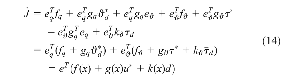
Proof. For (8), choosing the Lyapunov function candidate as $J = e^{T} e / e^{T} e 2 2$ and taking the derivative along with (9) and (11), one obtains

\begin{matrix} \overset{\cdot}{J} = e_{q}^{T} f_{q} + e_{q}^{T} g_{q} ϑ_{d}^{*} + e_{q}^{T} g_{q} e_{ϑ} + e_{ϑ}^{T} f_{ϑ} + e_{ϑ}^{T} g_{ϑ} τ^{*} \\ - e_{ϑ}^{T} g_{q}^{T} e_{q} + e_{ϑ}^{T} k_{ϑ} {\bar{τ}}_{d} \\ = e_{q}^{T} (f_{q} + g_{q} ϑ_{d}^{*}) + e_{ϑ}^{T} (f_{ϑ} + g_{ϑ} τ^{*} + k_{ϑ} {\bar{τ}}_{d}) \\ = e^{T} (f (x) + g (x) u^{*} + k (x) d) \end{matrix}

(14)

Comparing (14) and (13), it can be seen that the control law $u^{*}$ for (13) and (8) is equivalent.

This completes the proof.

Remark 1. If control law $u^{*}$ exists, it will be the integrated kinematic and dynamic control law as opposed to back-stepping control laws where kinematic and dynamic control inputs are separated.

Remark 2. $f (x)$ represents system’s drift tracking dynamics and $d$ is the bounded unknown disturbance according to Property 3.

Fact 1. $‖ q ‖ \geq ‖ q - q_{d} ‖ = ‖ e ‖$ , thus by Property 4, $f (x)$ is constrained by $f (x) \leq - {\bar{m}}_{min}^{- 1} c_{max} ‖ e ‖$ .

RL-based intelligent tracking control algorithm

According to the defined objective, applying and developing the policy iteration (PI) algorithm of RL for system (13) is an appropriate choice. RL can be used to learn online HJB solutions for optimal control problems (Vamvoudakis and Lewis, 2010) and HJI solutions for the H_∞ optimal problems (Vamvoudakis and Lewis, 2011; Vamvoudakis et al., 2011). Define a value function based on the H_∞ tracking performance index function object to (13) (Chen et al., 1998; Chen et al., 2009; Luy et al., 2010):

V = \int_{t}^{\infty} r (e (τ), u (τ), d (τ)) d τ

(15)

where $r (e, u, d) = Q (e) + u^{T} Ru - ρ^{2} d^{T} d$ , with $Q (e)$ is positive definite, i.e. $\forall e \neq 0$ $Q (e) > 0$ and $e = 0$ , $\Rightarrow Q (e) = 0$ , $u$ is the admissible control input that minimizes $V$ while $d$ tries to maximize $V$ (Dierks and Jagannathan, 2010; Vamvoudakis and Lewis, 2011), $R$ is a symmetric positive definite matrix, $ρ > ρ^{*}$ is the prescribed disturbance attenuation level, where $ρ^{*} > 0$ is the minimum gain of $ρ$ for which the stability of closed-loop tracking system (13) is guaranteed (Van Der Shaft, 1992). Define the Hamiltonian of (15) associated with u and d as

H (e, u, d, V_{e}) = r (e, u, d) + V_{e}^{T} (f (x) + g (x) u + k (x) d)

(16)

where $V_{e} = \partial V (e) / \partial V (e) \partial e \partial e$ . There exists a minimum non-negative local smooth solution of (16) (Dierks and Jagannathan, 2010; Vamvoudakis et al., 2011). If $V_{e}^{*}$ is that solution and (13) is locally detectable, then the Nash equilibrium solutions in term of $V_{e}^{*}$ can be found by the stationary condition of (16), i.e. $u^{*}$ and $d^{*}$

u^{*} (e) = - \frac{1}{2} R^{- 1} g^{T} (x) V_{e}^{*}

(17)

d^{*} (e) = \frac{1}{2 ρ^{2}} k^{T} (x) V_{e}^{*}

(18)

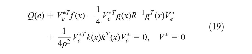
where $V_{e}^{*} = \partial V^{*} (e) / \partial e$ . The tracking HJI equation is obtained by substituting (17) and (18) into (16):

\begin{matrix} Q (e) + V_{e}^{* T} f (x) - \frac{1}{4} V_{e}^{* T} g (x) R^{- 1} g^{T} (x) V_{e}^{*} \\ + \frac{1}{4 ρ^{2}} V_{e}^{* T} k (x) k^{T} (x) V_{e}^{*} = 0, V^{*} = 0 \end{matrix}

(19)

Solutions HJI of (19) can be learned without explicit knowledge of the system’s drift dynamics by an integral RL-based PI algorithm where three NNs for the actor critic, which are the same structure, are required (Vamvoudakis et al., 2011). Using three NNs may lead to the computational complexity and resource consumption when applying for multivariable systems such as the WMR system defined earlier. Therefore, in this paper, the new actor critic scheme is proposed for the tracking problem using only one NN with the purpose of reducing the cost of computation and storage resources. The critic with the NN to approximate the optimal value function (15) is defined as

V^{*} (e) = W^{T} Φ (e) + ε (e)

(20)

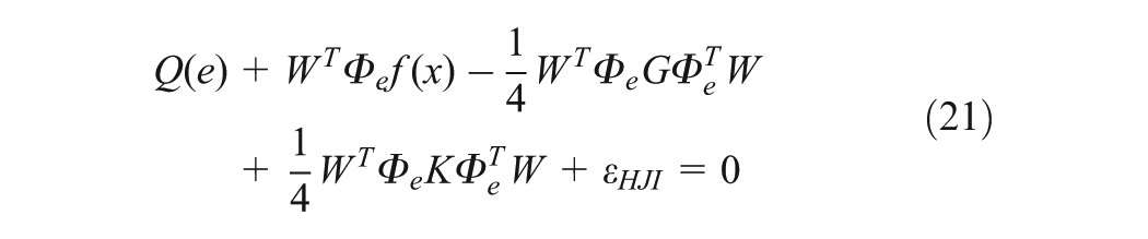
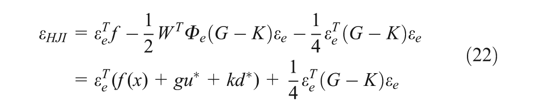
where $Φ (e) : ℜ^{n} \to ℜ^{N}$ is the activation function vector, N is the number of neurons in the hidden layer, $ε (e)$ is the NN approximation error and $W \in ℜ^{N}$ is the NN ideal weight vector. $Φ (e)$ can be selected such that, $N \to \infty, ε (e) \to 0$ and $ε_{e} (e) = \partial ε (e) / \partial ε (e) \partial e \partial e \to 0$ , and for fixed N, $‖ ε (e) ‖ < ε_{max}$ , $‖ ε_{e} (e) ‖ < ε_{e max}$ where $ε_{max}$ and $ε_{e max}$ are positive constants (Finlayson, 1990). Let us substitute (19), (20) into (16) to obtain the NN-based HJI equation

\begin{matrix} Q (e) + W^{T} Φ_{e} f (x) - \frac{1}{4} W^{T} Φ_{e} G Φ_{e}^{T} W \\ + \frac{1}{4} W^{T} Φ_{e} K Φ_{e}^{T} W + ε_{HJI} = 0 \end{matrix}

(21)

where $G = g R^{- 1} g^{T}, K = k k^{T} / k k^{T} ρ^{2} ρ^{2}$ , $Φ_{e} (e) = \partial Φ (e) / \partial Φ (e) \partial e \partial e$ and $ε_{HJI}$ is the residual error formed by the NN approximation error

\begin{matrix} ε_{HJI} = ε_{e}^{T} f - \frac{1}{2} W^{T} Φ_{e} (G - K) ε_{e} - \frac{1}{4} ε_{e}^{T} (G - K) ε_{e} \\ = ε_{e}^{T} (f (x) + g u^{*} + k d^{*}) + \frac{1}{4} ε_{e}^{T} (G - K) ε_{e} \end{matrix}

(22)

when $N \to \infty$ , $ε_{HJI}$ converges uniformly to zero. For fixed $N$ , $ε_{HJI}$ is bounded on a compact set (Vamvoudakis et al., 2011).

Fact 2. According to Properties 5 and 6, $G$ is bounded such that $0 \leq G_{min} \leq G \leq G_{max}$ , $G_{min} = g_{min}^{2} σ_{max} (R)$ and $G_{max} = g_{max}^{2} σ_{min} (R)$ , with $σ_{min} (R)$ and $σ_{min} (R)$ are the largest and smallest eigenvalues of R, respectively.

Fact 3. According to Properties 7, K is bounded such that $0 \leq K_{min} \leq K \leq K_{max}$ , $K_{min} = k_{min}^{2} / k_{min}^{2} ρ^{2} ρ^{2}$ , $K_{\max} = k_{\max^{2}} / ρ^{2}$ .

Assumption 1. The closed-loop tracking dynamics of WMR is bounded such that $‖ f (x) + g u^{*} + k d^{*} ‖ \leq γ_{\max}$ for the positive constant $γ_{max}$ .

The ideal weight vector $W$ (20) is unknown, thus $V (e)$ is valued by

\hat{V} (e) = {\hat{W}}^{T} Φ (e)

(23)

Then, the estimated control and disturbance laws become

\hat{u} (e) = - \frac{1}{2} R^{- 1} g {(x)}^{T} Φ_{e}^{T} \hat{W}

(24)

\hat{d} (e) = \frac{1}{2 ρ^{2}} k^{T} (x) Φ_{e}^{T} \hat{W}

(25)

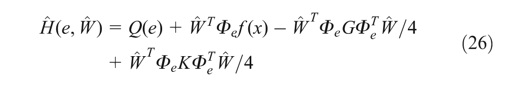
The approximate Hamiltonian is obtained by substituting (23), (24) and (18) into (16)

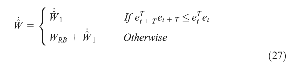
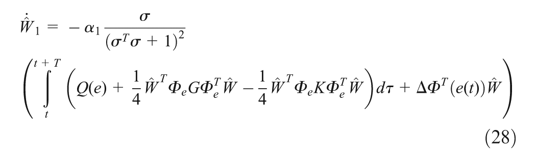
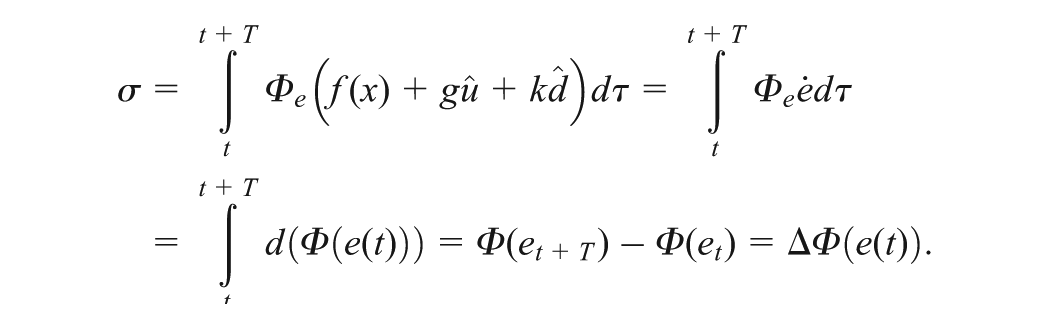
\begin{matrix} \hat{H} (e, \hat{W}) = Q (e) + {\hat{W}}^{T} Φ_{e} f (x) - {\hat{W}}^{T} Φ_{e} G Φ_{e}^{T} \hat{W} / 4 \\ + {\hat{W}}^{T} Φ_{e} K Φ_{e}^{T} \hat{W} / 4 \end{matrix}

(26)

Observing Equations (21) and (26), it is straightforward to see that $\hat{W}$ should be tuned to minimize the subject error function related to $\hat{H} (e, \hat{W})$ . To design a tuning law for $\hat{W}$ that does not depend on $f (x)$ , the error function is chosen as $E = \frac{1}{2} e_{H}^{T} e_{H}$ , where $e_{H} = \int_{t}^{t + T} \hat{H} (e, \hat{W}) d τ$ with T>0 is a chosen sampling time. Then, the tuning law becomes $\overset{\cdot}{\hat{W}} = - α_{1} \partial E / \partial E \partial \hat{W} \partial \hat{W}$ . In addition, due to the approximation error during online learning, it is desired to design the tuning law of $\hat{W}$ such thatit not only minimizes $E$ but also guarantees the stabilization of the system, concurrently. If more than one NN is used, the tuning law of the critic NN is responsible for minimizing $E$ , while the tuning laws of actor NNs guarantee the robust stability for the overall system. In our case, only one NN is used and thus both objectives must be intergraded into one, i.e.

\overset{\cdot}{\hat{W}} = {\begin{matrix} {\overset{\cdot}{\hat{W}}}_{1} & If e_{t + T}^{T} e_{t + T} \leq e_{t}^{T} e_{t} \\ W_{RB} + {\overset{\cdot}{\hat{W}}}_{1} & Otherwise \end{matrix}

(27)

where $e_{t} = e (t)$ , $e_{t + T} = e (t + T)$ , and

\begin{matrix} {\overset{\cdot}{\hat{W}}}_{1} = - α_{1} \frac{σ}{{(σ^{T} σ + 1)}^{2}} \\ (\int_{t}^{t + T} (Q (e) + \frac{1}{4} {\hat{W}}^{T} Φ_{e} G Φ_{e}^{T} \hat{W} - \frac{1}{4} {\hat{W}}^{T} Φ_{e} K Φ_{e}^{T} \hat{W}) d τ + Δ Φ^{T} (e (t)) \hat{W}) \end{matrix}

(28)

W_{RB} = - \frac{α_{2}}{2} Φ_{e} (G - K) e

(29)

where

\begin{array}{l} σ = \int_{t}^{t + T} Φ_{e} (f (x) + g \hat{u} + k \hat{d}) d τ = \int_{t}^{t + T} Φ_{e} \dot{e} d τ \\ = \int_{t}^{t + T} d (Φ (e (t))) = Φ (e_{t + T}) - Φ (e_{t}) = Δ Φ (e (t)) . \end{array}

It will be shown in the proof of Theorem 1 that along with ${\overset{\cdot}{\hat{W}}}_{1}$ in (27) and the added term, $W_{RB}$ , we will guarantee that the closed-loop system is uniform ultimately bounded (UUB; Lewis et al., 1999) when the behaviour of the overall system becomes unstable.

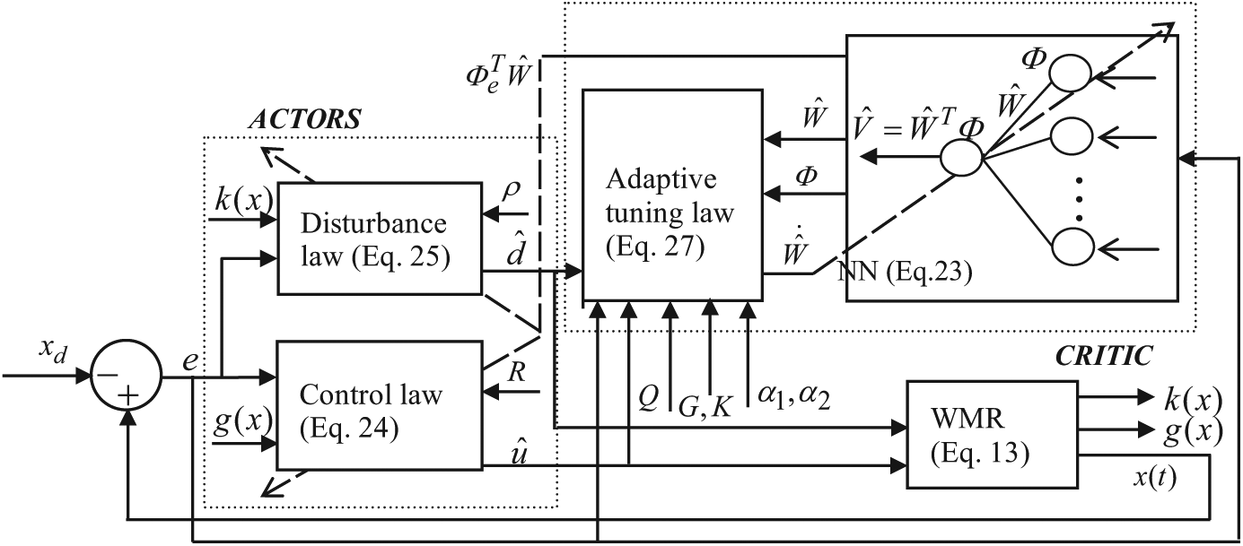
The proposed actor critic structure to learn and feedback control online is shown in Figure 1. It can be seen that the adaptive tuning law for the single NN in (27) is applied to update the NN weight such that the error function of approximate Hamiltonian in (26) is minimized and it does not involve the system’s drift dynamics, so the intelligent tracking control law defined previously can be obtained.

Figure 1.

The proposed actor critic structure.

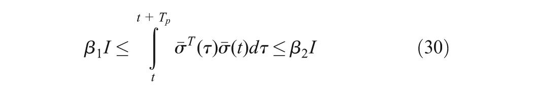
To guarantee the convergence of $\hat{W}$ , the control inputs and disturbance must be fully explored by adding the noise probe to $\hat{u} (e)$ and $\hat{d} (e)$ . That means the Persistence of Excitation (PE) condition in the interval $[t, t + T_{P}]$ with $T_{P} > 0$ , for all $t$ must be satisfied (Vamvoudakis et al., 2011)

β_{1} I \leq \int_{t}^{t + T_{p}} {\bar{σ}}^{T} (τ) \bar{σ} (t) d τ \leq β_{2} I

(30)

where $β_{1}$ and $β_{2}$ are positive constants, $\bar{σ} = 1 / (σ^{T} σ + 1)$ and I is the identity matrix with the appropriate dimension.

Theorem 1. Let the tracking dynamics of WMR be given by (13) with the objective tracking HJI equation (19), critic NN be given by (20), the tuning law for critic be defined in (27) and the intelligent tracking control and disturbance laws to approximate the $H_{\infty}$ optimal tracking cost function (15) be defined in (24) and (25), $\bar{σ}$ is satisfied with the condition PE (30). Then, the closed-loop system state $e$ and the NN error $\tilde{W}$ are UUB with the limited number of hidden layer units. Furthermore, the approximation errors of control input and worst-case disturbance are bounded such that $‖ u^{*} - \hat{u} ‖ < ε_{u}$ , $‖ d^{*} - \hat{d} ‖ < ε_{d}$ for small positive constants $ε_{u}$ , $ε_{d}$ .

Proof. See Appendix A.

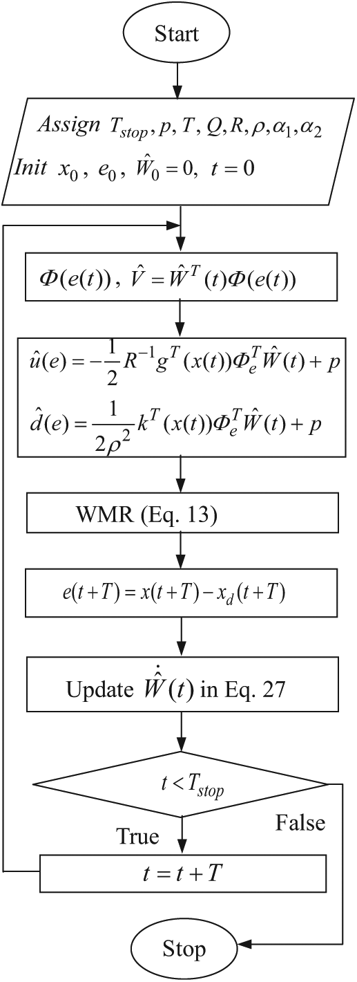
The proposed algorithm is represented by the block diagram in the Figure 2. $T_{stop}$ is the time to stop the algorithm, p is the noise probe and the other parameters are mentioned before.

Figure 2.

The block diagram of the algorithm.

Simulation results

To verify the proposed algorithm, two numerical simulations are offered. In the former, a non-linear system is learned and controlled by the proposed algorithm using one NN in comparison with another one using three NNs (Vamvoudakis et al., 2011). In the latter, the proposed algorithm is applied for the WMR.

Non-linear system

Consider the non-linear system with disturbance inputs, with a quadratic cost defined as in Vamvoudakis et al. (2011):

\overset{\cdot}{x} = f (x) + g (x) u + k (x) d

(31)

where $f (x) = {[- x_{1} + x_{2}, - x_{1}^{3} - x_{2}^{3} + 0.25 x_{2} {(\cos (2 x_{1} + 2))}^{2} - (0.25 / 0.25 ρ^{2} ρ^{2}) x_{2} {(\sin (4 x_{1} + 2))}^{2}]}^{T}$ $g (x) = {[0, \cos (2 x_{1}) + 2]}^{T}$ and $k (x) = {[0, \sin (4 x_{1}) + 2]}^{T}$ . We simulate in turn the non-linear system by the proposed algorithm using one NN and the algorithm in Vamvoudakis et al. (2011)using three NNs. To be comparable, the optimal tracking problem in the paper is transformed to the optimal control problem as Vamvoudakis et al. (2011), by defining the vector of tracking error as $e = x - x_{d}$ , where $x_{d} = 0$ . In this case, the tracking dynamic Equation (13) is in the form of Equation (31).

In both algorithms, one selects $Q = [\begin{matrix} 1 & 0 \\ 0 & 1 \end{matrix}]$ , $R = 1$ , $ρ = 8$ , $α_{1} = 50$ , $α_{2} = 0.01$ , $T = 0.05$ and T_stop=80 s. The optimal value function is $V^{*} (x) = \frac{1}{4} x_{1}^{4} + \frac{1}{2} x_{2}^{2}$ , so the optimal inputs are $u^{*} (x) = - \frac{1}{2} (\cos (2 x_{1}) + 2) x_{2}$ and $d^{*} (x) = - \frac{1}{2 ρ^{2}} (\sin (4 x_{1}) + 2) x_{2}$ by theory. The NN activation function vectors are defined as $Φ (x) = {[x_{1}^{2} x_{2}^{2} x_{1}^{4} x_{2}^{4}]}^{T}$ and the weight vector of critic NNs are defined as ${\hat{W}}^{1} = {[{\hat{W}}_{1}^{1} {\hat{W}}_{2}^{1} {\hat{W}}_{3}^{1} {\hat{W}}_{4}^{1}]}^{T}$ for the algorithm using one NN and ${\hat{W}}^{3} = {[{\hat{W}}_{1}^{3} {\hat{W}}_{2}^{3} {\hat{W}}_{3}^{3} {\hat{W}}_{4}^{3}]}^{T}$ for one using three NNs. All initial values of weights are zeros. The other parameters for three NNs can be seen in Vamvoudakis et al. (2011).

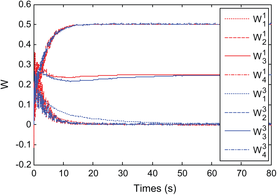
The convergence of critic parameters of both are shown in Figure 3. In the algorithm using one NN, all parameters converge at about 20 s with optimal values ${\hat{W}}^{1} = {[\begin{matrix} 0.006 & 0.5 & 0.2483 & 0 \end{matrix}]}^{T}$ , while using three NNs, they converge slower, at about 50 s with optimal values ${\hat{W}}^{3} = {[\begin{matrix} 0.005 & 0.5 & 0.2437 & 0 \end{matrix}]}^{T}$ . In addition, the parameters of the NNs for the actor and disturbance in the algorithm using three NNs also converged to the optimal approximate values (see Vamvoudakis et al., 2011, for more detail). Thus, using (24) and (25), both algorithms give similarly the optimal control inputs $u^{*} (x)$ and the optimal disturbance inputs $d^{*} (x)$ . However, it can be seen that using single NN, the proposed algorithm has reduced the complexity and resources, and given the convergence speed faster than the algorithm using three NNs.

Figure 3.

Convergence of parameters of the critic neural networks (NNs) in algorithms using one and three NNs.

Wheeled mobile robot

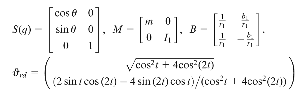
Consider the WMR defined above. With the notation introduced before, state vectors and parameters of WMR are $q = {[x, y, θ]}^{T}$ , $ϑ = {[v, ω]}^{T}$ , $r_{1} = 0.05 m$ , $b_{1} = 0.5 m$ and $l = 0$ , $m = 10 kg$ , $I_{1} = 5 kg . m^{2}$ where $m$ and $I_{1}$ denote the value of the mass and the moment of inertia of the platform, motors and wheels, respectively. Note that with the designed robust adaptive control law, WMR parameters can change online in bounded domains. One assumes that the control torques $τ$ applied to DC motor-mounted gearboxes are statically related to the voltage input by a constant so the electrical dynamics of the motors can be included in the general disturbance $τ_{d}$ such that $‖ τ_{d} ‖ \leq 3 N . m$ . If the WMR matrices and desired velocities of the reference robot are defined as $C (q, \dot{q}) \dot{q} = m l^{2} {\dot{θ}}^{2} {[\cos θ, \sin θ, 0]}^{T}$ ,

\begin{array}{l} S (q) = [\begin{matrix} \cos θ & 0 \\ \sin θ & 0 \\ 0 & 1 \end{matrix}], M = [\begin{matrix} m & 0 \\ 0 & I_{1} \end{matrix}], B = [\begin{matrix} \frac{1}{r_{1}} & \frac{b_{1}}{r_{1}} \\ \frac{1}{r_{1}} & - \frac{b_{1}}{r_{1}} \end{matrix}] \\ ϑ_{r d} = (\begin{matrix} \sqrt{\cos^{2} t + 4 \cos^{2} (2 t)} \\ (2 \sin t \cos (2 t) - 4 \sin (2 t) \cos t) / (\cos^{2} t + 4 \cos^{2} (2 t)) \end{matrix}) \end{array}

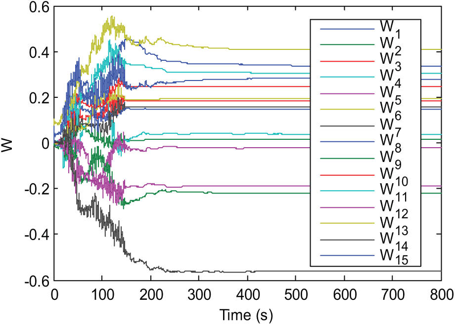
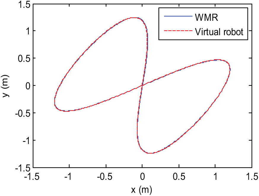
Then $f (x)$ , $g (x)$ and $k (x)$ are identified by changing these parameters to the formulations in Definitions 1 and 3. The smooth desired eight-shaped trajectory $q_{d} = {[x_{d}, y_{d}, θ_{d}]}^{T}$ is generated by $ϑ_{rd}$ and satisfied the constraint in Definition 2. The weight vector of critic NN is defined as $\hat{W} = {[{\hat{w}}_{1}, {\hat{w}}_{2}, \dots, {\hat{w}}_{15}]}^{T}$ , whose initial values are zeros. The adaptive gains are selected as $α_{1} = 100$ and $α_{2} = 0.01$ . The activation function vector of critic NN with 15 elements is chosen as $Φ (e) = {[e_{x}^{2}, e_{x} e_{y}, e_{x} e_{θ}, e_{x} e_{ϑ}, e_{x} e_{ω}, e_{y}^{2}, e_{y} e_{θ}, e_{y} e_{ϑ}, e_{y} e_{ω}, e_{θ}^{2}, e_{θ} e_{ϑ}, e_{θ} e_{ω}, e_{ϑ}^{2}, e_{ϑ} e_{ω}, e_{ω}^{2}]}^{T}$ One selects $R = I \in ℜ^{4 \times 4}$ , $R = I \in ℜ^{4 \times 4}$ and $ρ = 5$ . The PE condition is applied by adding the noise $e^{- 0.005 t} rand (t)$ to the control inputs and disturbance where $rand (t)$ generates random signals in the range [−1,1]. The desired position vector of the virtual robot is initial at $q_{d} (0) = {[x_{d}, y_{d}, θ_{d}]}^{T} = {[0, 0, π / 6]}^{T}$ . The initial position and velocities of WMR are $q (0) = {[0.5, 0.5, 0]}^{T} m$ , $ϑ (0) = {[0, 0]}^{T}$ , respectively. The parameter T is chosen as $0.01 s$ and $T_{stop} = 800 s$ .

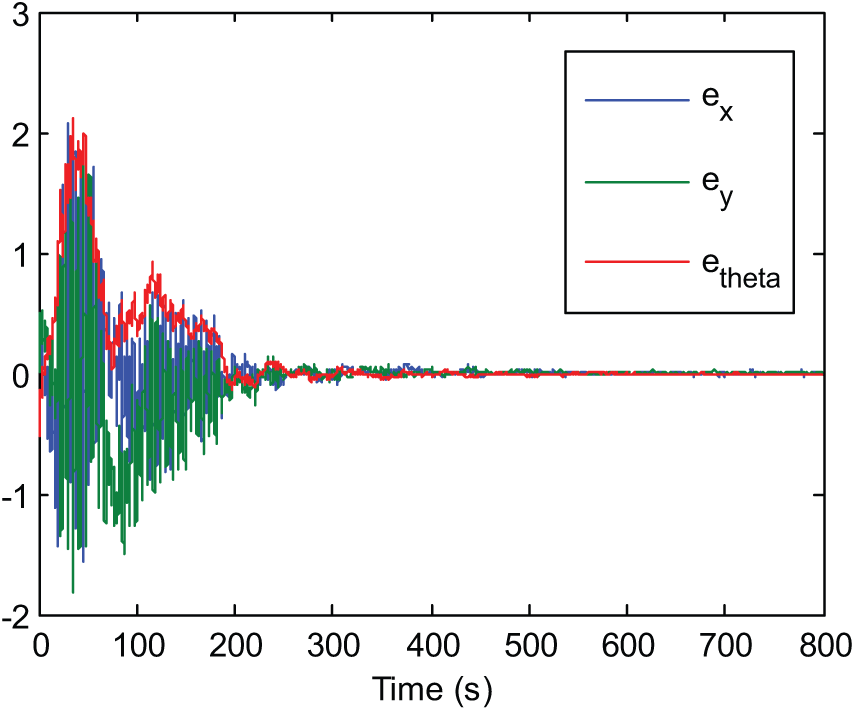
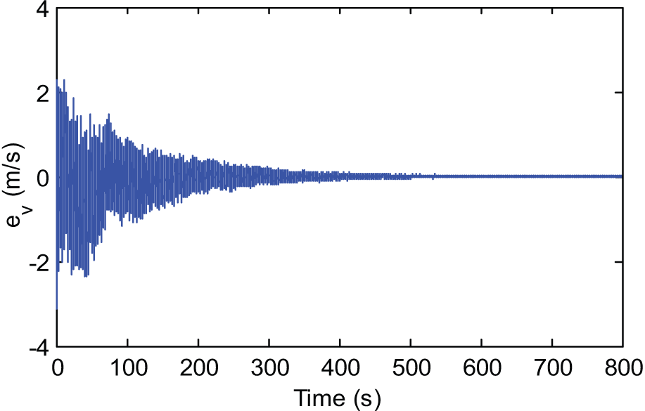
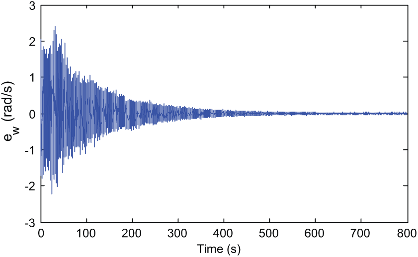
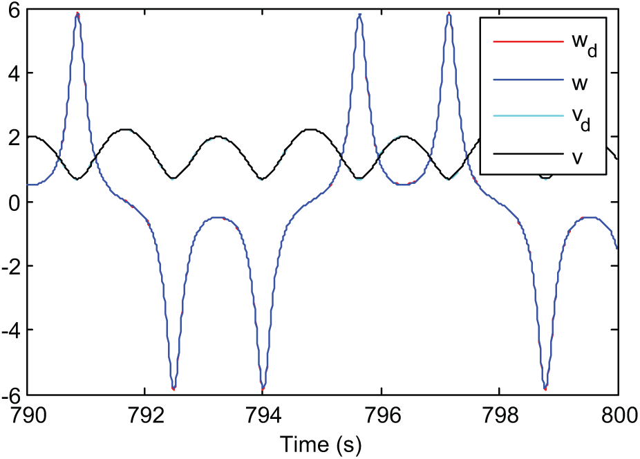
The convergence of critic parameters is shown in Figure 4. It can be seen that almost parameters converge after 300 s. The PE noise can be cancelled any time after that; here it is after 500 s. The evolution of the posture tracking errors during the simulation is presented in Figure 5. Although affected by input disturbances, the errors still converge closely to zero. Posture tracking of the WMR versus the reference robot by the designed robust direct adaptive controller is shown in Figure 6. The evolution of tracking errors between virtual control velocities and the WMR during simulation is shown in Figures 7 and 8, while Figure 9 represents the actual and virtual velocities.

Figure 4.

Convergence of parameters of the critic neural network (NN).

Figure 5.

Evolution of the posture tracking errors during simulation.

Figure 6.

Posture of wheeled mobile robot (WMR) with input disturbances.

Figure 7.

Evolution of the linear velocity tracking error.

Figure 8.

Evolution of the rotation velocity tracking error.

Figure 9.

Actual and virtual velocities with input disturbance.

Conclusion

The paper presents a new method for designing an integrated kinematic and dynamic intelligent tracking control algorithm for a WMR. The designed algorithm is a synchronous policy iteration using the actor critic structure with a single NN. Closed-loop dynamic tracking errors and critic parameters are proved to show UUB stability during the online learning. The optimal value function, the robust direct adaptive control input and worst-case disturbance are converged to the optimal approximate values.

Footnotes

Appendix A: proof

Funding

This research received no specific grant from any funding agency in the public, commercial, or not-for-profit sectors.

References

Abu-Khalaf

Lewis

(2005) Nearly optimal control laws for nonlinear systems with saturating actuators using a neural network HJB approach. Automatica 41(5): 779–791.

Chen

Uang

Tseng

(1998) Robust tracking enhancement of robot systems including motor dynamics: a fuzzy-based dynamic game approach. IEEE Transactions on Fuzzy Systems 6(4): 538–552.

Chen

Wang

. (2009) Moving horizon H_∞ tracking control of wheeled mobile robots with actuator saturation. IEEE Transactions on Control Systems Technology 17(2): 449–457.

Chwa

(2010) Tracking control of differential-drive wheeled mobile robots using a backstepping-like feedback linearization. IEEE Transactions on Systems, Man, and Cybernetics—Part A: Systems and Humans 40(6): 1285–1295.

Dierks

Jagannathan

(2010) Optimal control of affine nonlinear continuous-time systems using an online Hamilton–Jacobi–Isaacs formulation. In: 49th IEEE Proceedings of the CDC2010 (pp. 3048–3053).

Fierro

Lewis

(1998) Control of a nonholonomic mobile robot using neural networks. IEEE Transactions on Neural Networks 4: 589–600.

Finlayson

(1990) The Method of Weighted Residuals and Variational Principles. New York: Academic Press.

Hornik

Stinchcombe

White

(1990) Universal approximation of an unknown mapping and its derivatives using multilayer feedforward networks. Neural Networks 3: 551–560.

Khoshnam

Alireza

Ahmadrez

(2011) Adaptive feedback linearizing control of nonholonomic wheeled mobile robots in presence of parametric and nonparametric uncertainties. Robotics and Computer-Integrated Manufacturing 27(1): 194–204.

10.

Lewis

Jagannathan

Yesildirek

(1999) Neural Network Control of Robot Manipulators and Nonlinear Systems. London: Taylor & Francis.

11.

Lin

Yang

(2008) Adaptive critic motion control design of autonomous wheeled mobile robot by dual heuristic programming. Automatica 44: 2716–2723.

12.

Luy

(2012) Reinforcement learning-based optimal tracking control for wheeled mobile robot. In: Proceeding of the IEEE International Conference on Cyber Technology in Automation, Control, and Intelligent Systems, pp. 371–376.

13.

Luy

Thanh

. (2010) Robust reinforcement learning-based tracking control for wheeled mobile robot. In IEEE Proceedings of the ICCAE2010, Vol. 1, pp. 171–176.

14.

Marvin

Simon

Liberato

(2009) Dual adaptive dynamic control of mobile robots using neural networks. IEEE Transactions on Systems, Man, and Cybernetics—part b: Cybernetics 39(1): 129–141.

15.

Miyasato

(2008) Adaptive H_∞ control of nonholonomic mobile robot based on inverse optimality. In: Proceedings of the American Control Conference, Seattle, WA, pp. 3524–3529.

16.

Mohareri

Dhaouadi

Rad

(2012) Indirect adaptive tracking control of a nonholonomic mobile robot via neural networks. Neurocomputing 88: 54–66.

17.

Vamvoudakis

Lewis

(2010) Online actor critic algorithm to solve the continuous-time infinite horizon optimal control problem. Automatica 46: 878–888.

18.

Vamvoudakis

Lewis

(2011) Multi-player non-zero-sum games: online adaptive learning solution of coupled Hamilton–Jacobi equations. Automatica 47: 1556–1569.

19.

Vamvoudakis

Vrabie

Lewis

(2011) Online learning algorithm for zero-sum games with integral reinforcement learning. Journal of Artificial Intelligence and Soft Computing Research 1(4): 315–332.

20.

Van Der Shaft

(1992) L2-gain analysis of nonlinear systems and nonlinear state feedback H_∞ control. IEEE Transactions on Automatic Control 37(6): 770–784.

21.

Vrabie

Pastravanu

Lewis

. (2009) Adaptive optimal control for continuous-time linear systems based on policy iteration. Automatica 45(2): 477–484.

22.

Zenon

Marcin

(2011) Discrete neural dynamic programming in wheeled mobile robot control. Communications in Nonlinear Science & Numerical Simulation 16. 2355–2362.