






Abstract
In this paper, a mixed method of model order reduction for a continuous-time single-input single-output system is presented. The denominator of a reduced-order model (ROM) is obtained by clustering the poles of the original high-order system using the Fuzzy C-Means clustering technique retaining some dominant poles. Having determined the denominator polynomial, numerator coefficients are found by Padé approximation by matching the desired number of time moments and Markov parameters. The ROM of the proposed method provides good approximation to the original system both in terms of transient and steady-state response.
Introduction
Mathematical models of large engineering systems are complex and of high dimension and therefore the analysis and design of the controller of such a system are quite tedious and costly. It is, therefore, desirable that a higher-order model is replaced with low-order model. There are number of practical industrial applications of model order reduction in checking performance certification in the area of aircraft components, air traffic, integrated circuits, micro systems, etc. A large variety of methods of model order reduction in the frequency domain as well as the time domain are available in the literature (Bandyopadhyay and Lamba, 1987; Enright and Kamal, 1980; Hutton and Friedland, 1975; Krishnamurthy and Seshadri, 1978; Safonov and Chiang, 2004; Salimbahrami et al., 2005; Shamash, 1974; Singh et al., 2004; Vittal Rao and Lamba, 1974). In spite of several methods available, no approach gives best result for all systems.
A very powerful method that involves simple algebraic calculations comprises continued fraction, moments matching and Padé approximation. However, the Padé method has a drawback that it may produce an unstable approximant for a given stable original system. Many methods, such as Routh-approximation and Routh–Padé approximants and impulse energy approximation (Lucas, 1988, 1992), have been suggested to ensure the stability of the reduced-order model (ROM).
Krylov subspace methods (Salimbahrami and Lohmann, 2002; Salimbahrami et al., 2005) are also found to be a quite popular tool for obtaining ROMs of very high-order linear time-invariant systems, which is relatively simple and cheap and can handle systems with a few thousand degrees of freedom, but the stability of the ROM may not be guaranteed. Rudnyi and Korvink (2006) reported various modern applications of model order reduction for industrial applications. In industrial applications finite element models are high dimensional. Using model order reduction techniques such as Singular Value Decomposition (SVD)–Krylov subspace with better computational properties for a static solution in ANSYS software for several thermal and structural models may be employed effectively. This is also useful in radio frequency micro-electromechanical systems (RF MEMSs) considered being a main building block of future generations of reconfigurable wireless terminals.
Recently, Wu and Zheng (2009) presented a paper on H∞ model reduction for a continuous-time linear system with time-varying delay. By applying the average dwell time approach and the piecewise Lyapunov function technique, delay-dependent/delay-independent sufficient conditions are proposed in terms of linear matrix inequality (LMI) to guarantee the exponential stability and the weighted H∞ performance for the error system. In another paper, Wu et al. (2009) considered H∞ model reduction for linear parameter-varying (LPV) systems with both discrete and distributed delays. The problem of model order reduction for systems with time-invariant delay is investigated by using the delay-dependent approach. Further, Wu et al. (2011) presented model approximation for discrete-time Takagi–Sugeno (T-S) fuzzy state-delay systems. In this paper, a given stable T-S fuzzy system is well approximated in an H∞ performance and also translated into a linear lower order system. Su et al. (2012) used H∞ model order reduction for T-S fuzzy stochastic systems in which attention is focused on the construction of a ROM, which not only approximates the original system well with an H∞ performance, but also translates it into a linear lower dimensional system.
Another important group of reduction algorithm is the eigenvalue preservation technique where important eigenvalues of the system are retained to find a stable lower-order model (Gopal and Mehta, 1982). Recently, pole clustering techniques (Gonzalez et al., 2002; Napoleon and Pavalakodi, 2011; Vishwakarma and Prasad, 2008) have become quite popular in the area of model order reduction as they are conceptually simple and very easy to implement.
The proposed method is a mixed method for model order reduction that combines pole clustering, retention of dominant poles and Padé approximation. In this paper, a technique of pole clustering called Fuzzy C-Means (FCM) clustering (Hammouda and Fakhareddine, 2000) is used to find the desired number of pole clusters. The denominator of the ROM is found by retaining the dominant pole and clustering the remaining poles using the FCM algorithm and the numerator is determined using Padé approximation. This paper is organized as follows: problem formulation is given in Section 2. Numerical examples and comparison of the proposed method with other well-known techniques is shown in Section 3 and the conclusion is in Section 4.
Problem formulation
Consider a stable single-input single-output (SISO) system described by the transfer function
or
The problem is to determine its stable reduced-order (rth-order) approximant:
or
where
Pole clustering
Clustering of data is a process by which a large amount of data is grouped into a smaller number of groups to facilitate its meaningful analysis by lowering dimensionality (two or three, maximum). Clustering methods are generally used for organizing and categorizing data to solve classification and pattern recognition problems. It can also be useful for data compression and model order reduction. A number of clustering techniques are available in the literature. K-Means and FCM clustering are the types that can be used if numbers of clusters are known a priori as is required in the case of model order reduction. These techniques are used in conjunction with radial basis function networks (RBFNs) and fuzzy modelling.
The K-Means or Hard C-Means (HCM) clustering (Napoleon and Pavalakodi, 2011) algorithm relies on finding the cluster centres by minimizing a cost function (or an objective function) of dissimilarity (or distance) measure (Hammouda and Fakhareddine, 2000). In most cases dissimilarity measure is chosen as the Euclidean distance and the cost function based on the Euclidean distance between a vector
where Ji is the cost function within group i.
The partitioned groups are defined by a c×n binary membership matrix
If the membership matrix uij is fixed, then the optimal centre
FCM clustering (Hammouda and Fakhareddine, 2000) is an improvement over HCM clustering. In FCM clustering each data point belongs to a cluster to a degree specified by a membership grade and it allows one piece of data to belong to two or more clusters. The membership matrix
The cost function for FCM is a generalization of Equation (5):
where uij is between 0 and 1;
The necessary conditions for Equation (9) to reach to its minimum are
and
The FCM algorithm (Hammouda and Fakhareddine, 2000) works iteratively through the preceding two conditions until no more improvement is noticed. In a batch mode operation, FCM determines the cluster centres
Step1: Initialize the membership matrix
Step 2: Calculate c fuzzy cluster centres
Step 3: Compute the cost function according to Equation (9). Stop if it is below a certain tolerance value or its improvement over previous iteration is below a certain threshold.
Step 4: Compute a new
The FCM algorithm starts by assigning random values to the membership matrix
The desired number clustered pole centres of the denominator poles of the high-order system (HOS) is determined using the FCM algorithm discussed as above. If all the poles to be clustered are real, the desired number of cluster centres
If m pairs of complex conjugate poles in the jth cluster are [(α1±jβ1), (α2±jβ2),…, (αm±jβm)]|, using the same algorithm for both real and imaginary parts separately the cluster pole centres are obtained as фcj = Acj±jBcj, where Acj and Bcj are the cluster centres of real poles and imaginary poles, respectively.
Determination of the denominator of the reduced-order model
The rth order denominator of the reduced model is obtained as follows.
The most dominant poles
Determination of the numerator of the reduced-order model
The numerator of the ROM is determined by using Padé Approximation. G(s) (1) is expanded around s = 0 and s = ∞ as
where
Similarly, Gr(s) is expanded around s = 0 and s = ∞ as
where
We seek a stable model for which following r equations are to be satisfied:
The time moments and Markov parameters are related with numerator and denominator coefficients as
In this case, with the requirement that
Using the above equations and selecting the desired number of time moments and Markov parameters of the original and the ROM to be matched, the modified numerator coefficients
Numerical examples
Example 1: consider a stable eighth-order system (Vishwakarma and Prasad, 2008a)
(t1 = 1.0000, t2 = 1.8645, t3 = −2.4889; M1 = 18, M2 = −134, M3 = 978)
It is desired to obtain a third-order model of the form
For this example, the dominant pole to be retained is −1. Using the FCM algorithm (see Section 2), the remaining two pole clusters are found to be −3.1630 and −6.8382 and the denominator of the ROM is obtained as
The numerator of the ROM is obtained using Equations (18) as
Thus, the ROM of the proposed method turns out to be
In Vishwakarma and Prasad (2008b), the authors used the modified inverse distance measure (IDM) for pole clustering, and the third-order reduced model is obtained as
The third-order approximant according to Lucas (1988) is given as
The step responses of the original system and ROMs are plotted in Figure 1 and it is clearly seen that the step response of the proposed approximant (25) is almost identical to that of the HOS (21), while the ROMs (26) and (27) show deviation from the original system. These findings are also confirmed by examining the Integral Square Error (ISE) given in Table 1.
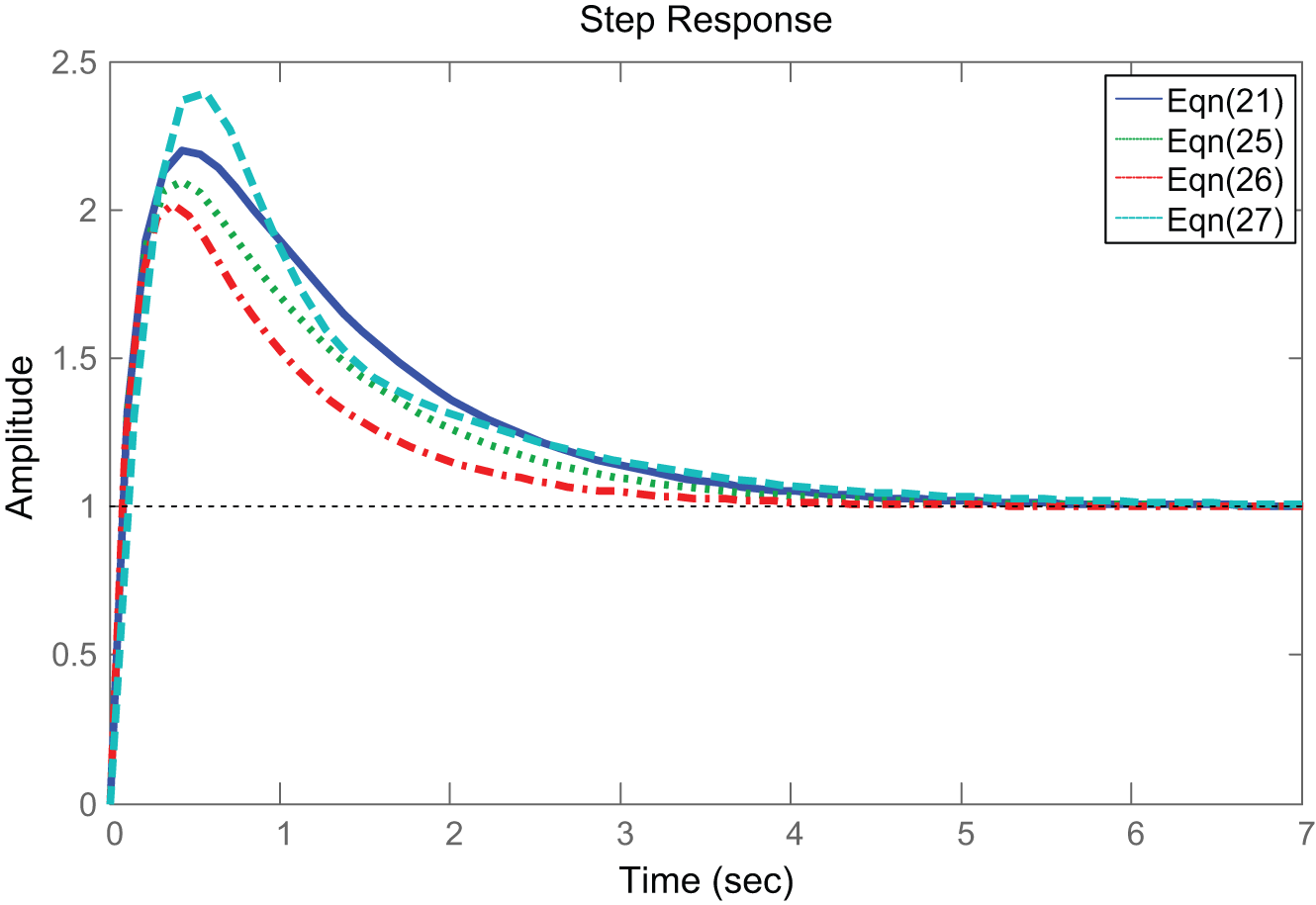
Step responses of the original and reduced-order models.
Comparison of results of different methods.
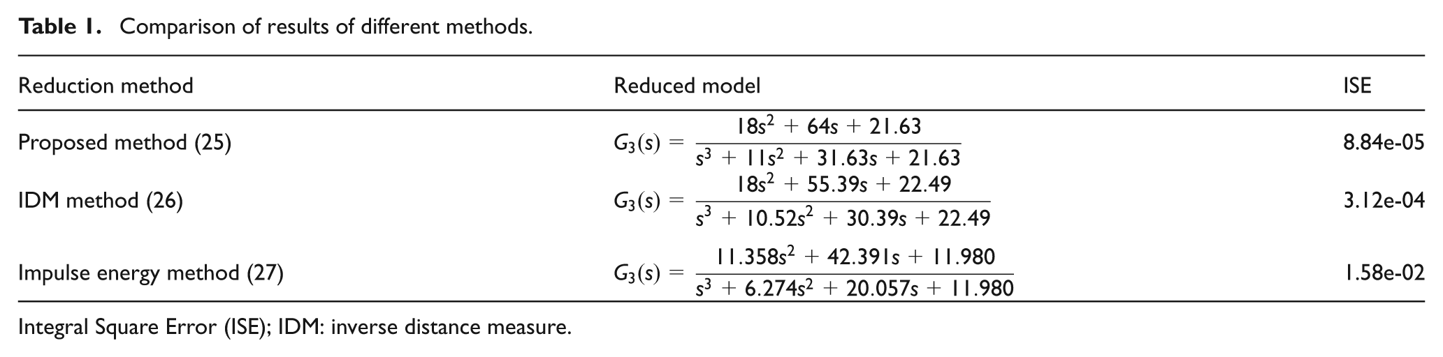
Integral Square Error (ISE); IDM: inverse distance measure.
Example 2: consider the transfer function (Srinivasan and Krishnan, 2010)
or
(t1 = 0.1007, t2 = −0.0256, t3 = 0.0078; M1 = 1, M2 = −47.3, M3 = 4290)
Using the proposed method, the third-order reduced model of the original system is found to be
Using modified the IDM (Vishwakarma and Prasad, 2008b) method, the third-order approximant comes out to be
The third-order approximant using the technique discussed by Srinivasan and Krishnan (2010) is
The step responses of the original system and ROMs are plotted in Figure 2. The relative superiority of the proposed ROM (30) over (31) and (32) is self-evident from the step responses and ISE given in Table 2.
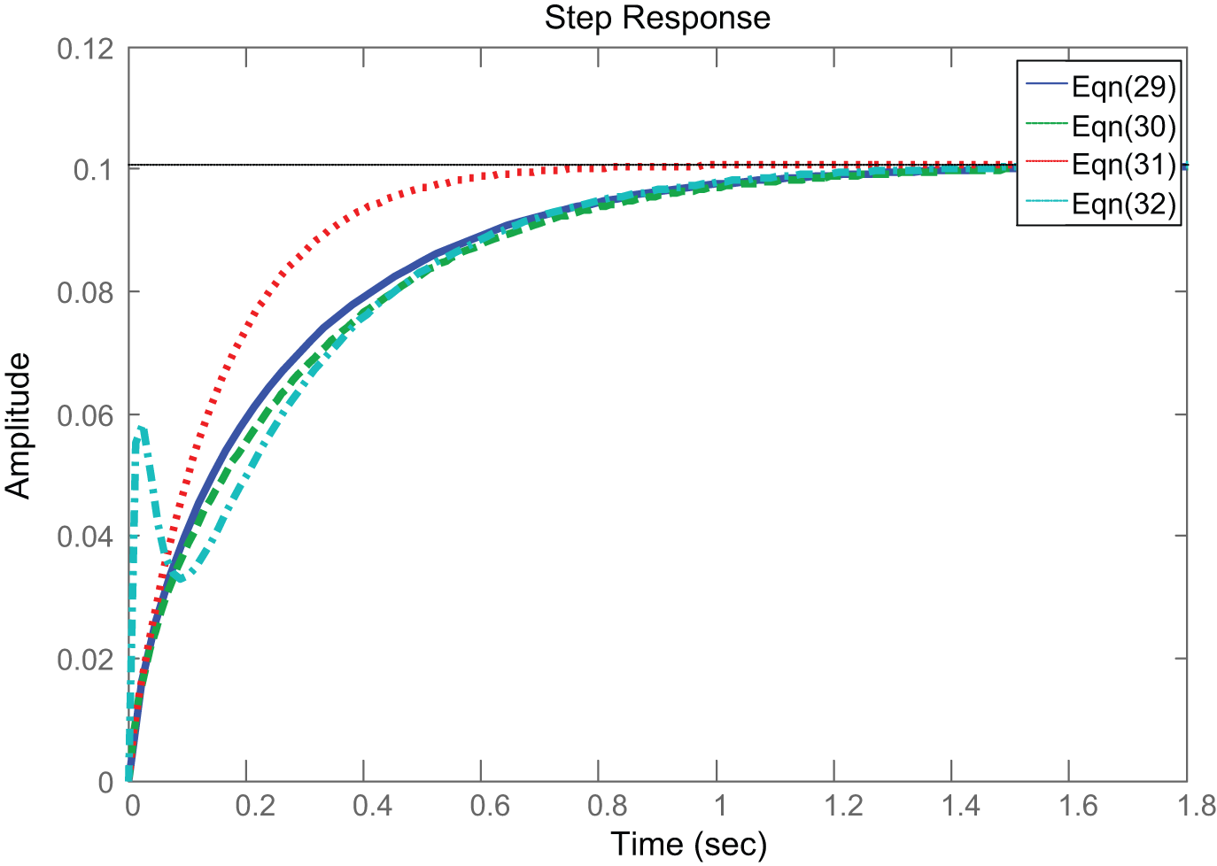
Step responses of the original and reduced-order models.
Comparison of results of different methods.
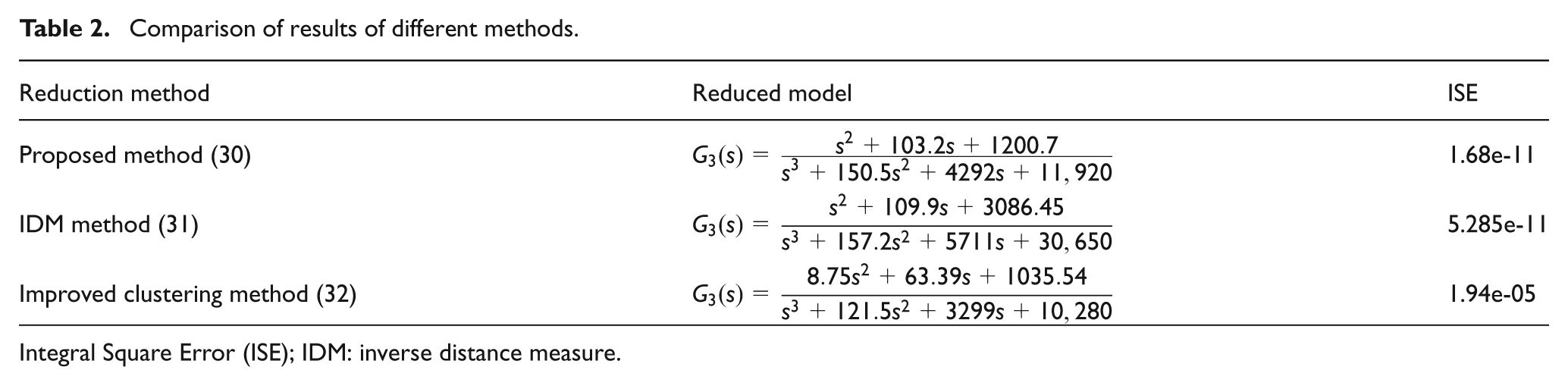
Integral Square Error (ISE); IDM: inverse distance measure.
Conclusion
In this paper, the stable ROM is obtained using the pole clustering-Padé method. The denominator is obtained by retaining the dominant pole and clustering the remaining poles of the original HOS. Having obtained the denominator, the numerator parameters are calculated by fully retaining the first r time moments/Markov parameters of the system. The proposed approach, therefore, leads to improved approximants. It is worth mentioning that the approach is ideally suited for large r (≥4). For low r (<4), the problem of identifying clusters of complex conjugate poles may possibly surface. This problem is open to investigation. Recently, the state-space techniques (Wu and Zheng, 2009) H∞ model reduction for linear switched time systems with time-varying delay and for LPV systems with distributed delay (Su et al., 2012; Wu et al., 2011), H∞ model reduction for discrete-time T-S fuzzy system time-delay systems and T-S fuzzy stochastic systems have emerged and are of considerable interest for reducing the order of the systems. It would be interesting to carry out a comparative study of the present approach and the state-space techniques.
Footnotes
Funding
This research received no specific grant from any funding agency in the public, commercial or not-for-profit sectors.