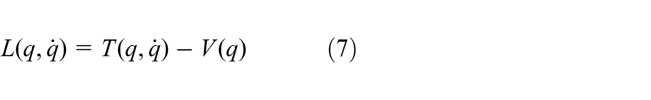
Dynamic simulation model of a biomimetic robotic fish with multi-joint propulsion mechanism

Abstract

In this paper, a biomimetic carangiform robotic fish is analysed based on dynamic and kinematic models. The carangiform fish can swim with features like high mobility, fast swimming and changing direction suddenly. Because it has these amazing features, a carangiform swimmer is modelled. Dynamic and kinematic models are analytically obtained to design a biomimetic carangiform robotic fish. The designed robotic fish consists of two parts: an anterior rigid body and a flexible tail, which is modelled as a four-joint propulsion mechanism, and each joint is driven by a servo motor. The dynamic model is developed in the MATLAB/Simulink environment using a Lagrange function and the state-space model is performed to linearize the obtained model. Each joint is controlled with conventional PID controller in the simulation. Furthermore, a solid model of the robotic fish prototype is drawn in SolidWorks and transferred to the MATLAB/Simmechanics environment, and the motion of the robotic fish is simulated using joint angles. Finally, experimental studies and simulation results show that a carangiform motion for autonomous swimming is developed and verified using controlled joint angles.

Keywords

Biomimetic design dynamic modelling Lagrange method multi-joint actuation robotic fish

Introduction

Biomimetics is a new branch of science that examines living forms in nature and mimics their systems to resolve human problems. At the same time, biomimetics is a term that expresses most human-made materials, mechanics and systems realized by mimicking nature. The increasing interest in these systems makes it more attractive for the transferring of technology between nature and engineering fields. Nowadays, living forms in nature are modelled for use in many fields, such as engineering systems, modern technology and robotics. As one topic, research on aquatic animals has increased and these animals have been mimicked to improve underwater vehicles and their locomotion mechanisms for better performance (Korkmaz, 2012; Korkmaz et al., 2011 2012; Sfakiotakis et al., 1999; Vepa, 2009).

It is known that fish have excellent swimming abilities in water and they are the best swimmers with features of manoeuvrability, capabilities of high speed and high efficiency. Fish swim using their bodies, fins and tails. In ichthyology, the swimming of fish is provided by both bending their bodies and/or caudal fins (BCF) and the motion of their median and/or paired fins (MPF) (Korkmaz et al., 2012; Yu et al., 2003). Such excellent swimming ability inspires robotic researchers to improve and develop the performance of an underwater vehicle (AUV) named a robotic fish.

In recent years, designs of the propulsion and manoeuvring mechanism inspired by fish have gained momentum in AUVs. Fish have fast and high manoeuvring ability with a generated thrust force such as undulation and oscillation propulsion. Observation on a real fish shows that the multi-joint propulsion is noiseless, faster and more manoeuvrable, with low power consumption according to the classic rotary propeller used in AUVs. A robotic fish designed with a multi-joint flapping mechanism is more efficient than the classic rotary propeller AUVs. According to Tong (2000), fish have swimming efficiency of over 80%, while classic rotary propellers have only between 40% and 50%. Furthermore, carangiform fish can turn rapidly with a radius of 10–30% of their body length, while classic AUVs may only change direction slowly with a radius of three times the body length (Triantafyllou and Triantafyllou, 1995). From the perspective of robotic research, a real fish is an appropriate structure to design and develop an autonomous AUV that is well suited for propulsion mechanism. These suitable features supply great benefits and the robotic fish can be used in many aquatic and military fields, such as detection of pollution, exploration of fish behaviours, coast guard, undersea robotic applications, etc (Liu and Hu, 2004; Liu et al., 2004; Yu et al., 2005; Zhang et al., 2007).

In 1994, the first robotic fish, named RoboTuna, was developed by MIT, and was known as the first free-swimming robotic fish in the world. It was equipped with features such as fish-like swimming through the eight-link flexible fin, and its drag reduction mechanism was researched experimentally (Yu et al., 2005). Triantafyllou and Triantafyllou (1995), and then Hirata (1999) examined the hydrodynamic performance of fish swimming and developed fish-type robots. The subsequently designed RoboPike enabled researchers to attempt to focus more on the design of a robotic fish (Yu et al., 2004). The Draper Laboratory created a novel AUV for vorticity control of an unmanned undersea vehicle, namely the VCUUV. It could avoid obstacles and had an up-down motion ability (Hu, 2006; Yu et al., 2005; Zhou et al., 2010). In addition, some universities developed micro robotic fish using various kinds of actuators (Chen et al., 2009; Ye et al., 2008; Zhang et al., 2008). Chen and colleagues (Chen et al., 2009; Zhou et al., 2010) designed specific pectoral fins for submerging and ascending motions. Zhang and colleagues designed a small robotic fish using an electrostatic film motor, named the Seidengyo, to control for high mobility performance (Zhang et al., 2008). A centimetre-scale robotic fish was realized by Ye at all (2008) to mimic a type of small crucian carp. It was designed using an ionic polymer metal composite (IPMC) actuator. In the 2000s, many kinds of robotic fish were developed by Yu et al. (2005, 2006, 2008) and a dynamic model for the three-dimensional (3-D) motion of robotic fish was investigated (Liu and Hu, 2004; Yu et al., 2008). Apart from these, intelligent control and optimization methods applied to robotic fish designs and various robotic fish prototypes were performed to achieve optimal fish-like motion with multi-joint mechanisms (Hu et al., 2006; Yu et al., 2005; Su et al., 2014). Recently, Hu (2006) designed a kind of carangiform robotic fish named G9 (9th Generation). It has the best swimming performance ever and is being exhibited in London County Hall Aquarium. However, an optimal propulsion model similar to a real fish for robotic fish has not yet been completed in this area (Hu, 2006; Qiu et al., 2007).

To imitate biological properties of a real fish in the autonomous AUVs, a suitable dynamic model must be obtained and a quantitative analysis for the designed mechanical structure must be performed. For this, various dynamic simulation models can be used to achieve an optimal model. Many theories have been suggested and built to explain fish swimming motions and its driving elements, i.e. two-dimensional (2-D) and 3-D waving plate theory (Stakiotakis et al., 1999; Yu et al., 2004), large-amplitude elongated body theory (Yu et al., 2005), some animations of fish for better performance (Hu, 2006), Lagrange and Lagrange–Euler functions (Zhou et al., 2008), and Newton–Euler methods (Yu et al., 2008).

The aim of this paper is to design a dynamic model of carangiform motion for a flexible multi-joint propulsion mechanism and autonomous swimming. The main principles for efficient thrust generation by a multi-joint propulsion mechanism are presented. Considering the carangiform motion, the designed robotic fish prototype consists of two parts: an anterior rigid body and a flexible tail fin, which includes a four-joint propulsion mechanism. The flexible body consists of hinge joints actuated by servo motors. Motion control of the robotic fish primarily depends on the kinematic model of the tail joints. The mechanical structure of the flexible tail is considered four revolving joints like a robot manipulator. The standard method to model the forward kinematics of the robot manipulator is the Denavit–Hartenberg (D-H) representation. Considering this approach, the kinematic model of the robotic fish is derived using D-H representation. The motion of the robotic fish is calculated by solving Lagrange’s equation analytically and the simulation model is established to perform carangiform motion in MATLAB/Simulink environment. Also, a solid model of the robotic fish prototype is drawn in SolidWorks and motion of the controlled system is simulated in MATLAB/Simmechanics environment using the joint angles. Comparing simulation results with experimental results, the dynamic model is validated.

The rest of this paper is organized as follows. In the next section, biologically inspired design is given and carangiform motion ability is described, followed by kinematic and dynamic models of the robotic fish. Then the realization of the robotic fish model is described, and simulation and experimental results are given. Finally, conclusions are presented.

Biologically inspired design

Carangiform motion

In terms of propulsion mechanisms, most fish, such as tuna, swim by bending their bodies into a form of a lateral sinusoidal wave and/or moving their caudal fins, namely BCF motion. Alternatively, some fish, such as the sunfish and many smaller fish, use alternative swimming motion that is produced using their median and pectoral fins, termed MPF. However, 15% of fish species swim with MPF, 80% of fish swim with BCF motion (Yu et al., 2005).

Both BCF and MPF modes can be separated in undulation and oscillation propulsions. In undulation, swimming motion is a form consisting of transition of a wave along the propulsion mechanism, while in oscillation, propulsion is generated either as reactions to a drag or via a lift mechanism. As shown in Figure 1, BCF swimming motion is usually categorized into anguilliform, subcarangiform, carangiform and thunniform modes, according to the wavelength and amplitude of the propulsive wave (Sfakiotakis et al., 1999; Wen et al., 2012). In this swimming mode, the propulsion mechanism produces a lateral water wave, which traverses from the fish body through the opposite direction and it is faster than the speed of the fish (Sfakiotakis et al., 1999).

Figure 1.

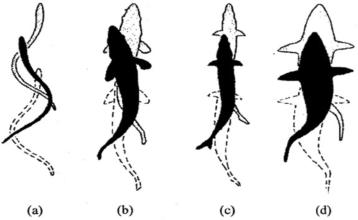
Classification of body and/or caudal fin (BCF) swimming motion by Sfakiotakis et al. (1999): (a) anguilliform (b) subcarangiform (c) carangiform (d) thunniform.

Recent studies on the robotic fish have primarily focused on the anguilliform and carangiform modes (Yu et al., 2005). During the anguilliform motion, the entire body moves in large-amplitude undulations. In the carangiform mode, this event is more pronounced and undulation occurs in more just two-thirds of the body. Also, the thrust force is produced by stiff caudal fin. Compared with carangiform with anguilliform, these swimmers are mostly faster, but have less manoeuvring ability due to their rigid bodies (Yu et al., 2005).

However, studies of the propulsion mechanism based on the carangiform swimmers are the most common, due to their easy design (Morgansen et al., 2001). In this paper, only carangiform motion is designed based on the biological structure of the real fish.

Simplified multi-joint propulsion model

For robotic fish design, there are several methods to produce propulsion, such as using caudal fins, paired pectoral fins, both caudal and pectoral fins, and many kinds of actuator materials. In the tail mechanism, one-joint to multi-joint design can be used and each joint is actuated by servo motors.

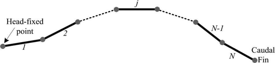
To simplify, a robotic fish is contemplated in planar motion in two dimensions and the z-axis can be neglected. In this case, the expected motion in a longitudinal direction is determined as the x-axis and the lateral direction is referred to as the y-axis (Morgansen et al., 2001). Based on the biological structure of carangiform mode, lateral motion, which is in the form of a travelling wave, smoothly increases, starting from nose to tail. The propulsive wave begins from the nose to tail by increasing amplitude, which behaves as lateral curvature in the spine (Liu and Hu, 2004). A physical model of carangiform motion is illustrated in Figure 2. The prepared robotic fish consists of two parts: an anterior rigid body and a flexible tail, which includes a four-joint propulsion mechanism. The anterior part is a streamlined body and the flexible body is designed by hinge joints actuated using servo motors. The caudal fin is connected to the tail by a peduncle whose influence is negligible in the hydrodynamic region (Yu et al., 2005).

Figure 2.

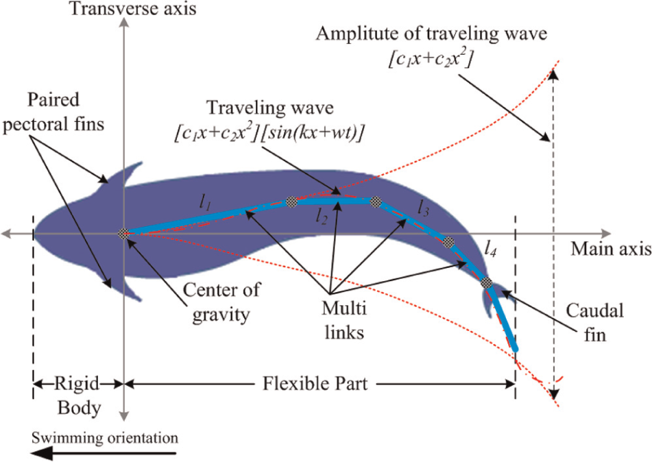
Physical model of the carangiform motion in lateral displacement.

This multi-joint model realized from the servo motors is considered a spine system of a real fish and each vertebra is a servo motor. Thus an artificial spine system is built. As a result, the robotic fish can approximate the swimming motion of a real fish; the tail joints determine the generated propulsion force.

The kinematic motion of the robotic fish can be described using a travelling wave function, originally suggested by Lighthill (1960), which is given by:

y_{body} (x, t) = (c_{1} x + c_{2} x^{2}) \sin (kx + wt)

(1)

where : k = 2 π / λ and w = 2 π f

(2)

In this equation, the travelling wave function is defined as lateral displacement at time t, x is the displacement along the main axis, and c₁ and c₂ are linear wave and quadratic wave amplitudes, respectively, which depend on the type of fish. k is the body wave number, λ is the body wavelength, w is the body wave frequency (rad/s) and f is the flapping frequency of the robotic fish. Equation (1) can be rewritten to obtain control angles for the multi-joint mechanism of the robotic fish actuated using four servo motors (Liu and Hu, 2004; Yu et al., 2008). Therefore, a discrete travelling wave function is described according to the following equation:

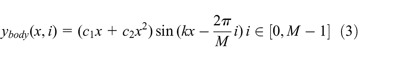
y_{body} (x, i) = (c_{1} x + c_{2} x^{2}) \sin (kx - \frac{2 π}{M} i) i \in [0, M - 1]

(3)

The function discretized from Equation (1) is computed in an analytic fitting solution and grouped as an M×N look-up table in the microcontroller. Here, N is the joint number. In Equation (3), i is the variable of the discrete travelling wave, y_body(x,i) for (i=0, 1, 2, …, M−1) in one oscillation period and M is the resolution of the discrete travelling wave. Figure 3 shows the discrete travelling waves for one period of the flapping mechanism with simulation parameters: M=18, c₁=0.3, c₂=0 and k=13.6. The values of these parameters were taken from the article of Liu and Hu (2004). The same values have been used by Yu and colleagues (2008), because the kinematic values of their robot are almost identical.

Figure 3.

The discrete travelling wave function.

It should be noted that parameters of the wave amplitudes c₁ and c₂ can be obtained from the observation of experimental studies and used to mimic real carangiform fish motion.

Modelling of the robotic fish

Recently, the design of artificial biological systems, which mimic real fish, have focused on fish-like motion mechanisms. Before create a biomimetic robotic fish, it is necessary to make a design scheme of the whole system. To mimic carangiform motion, a feasible mathematical model should be established with both kinematic and dynamics parameters. Based on the above mathematical models, a realistic design can be achieved, which provides an engineering guide to realize the biomimetic robotic fish.

Kinematic model of the robotic fish

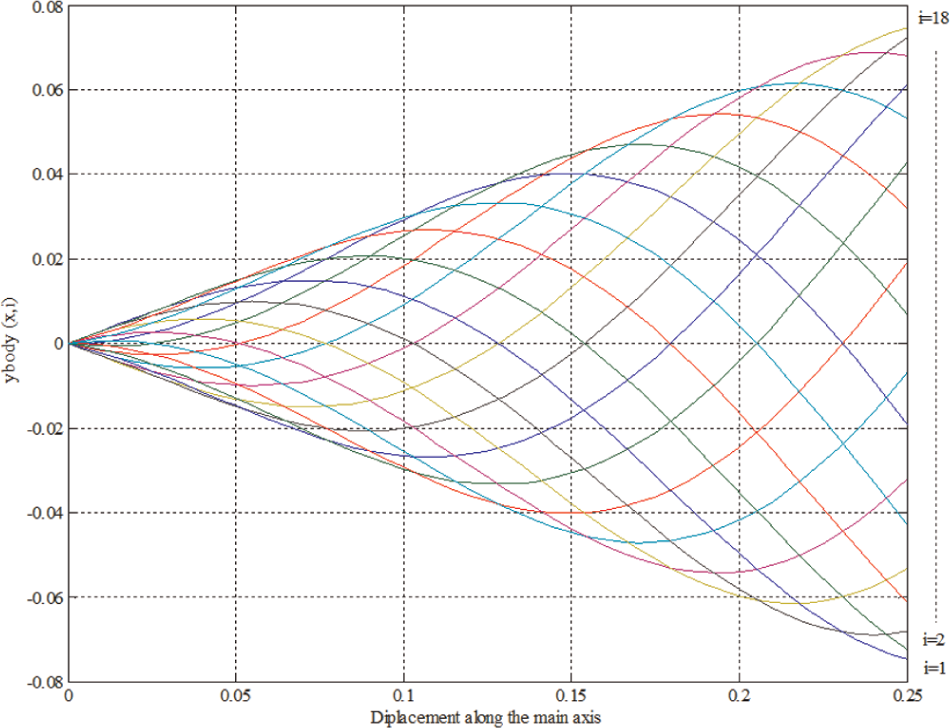
The designed robotic fish consists of the rigid body and a flexible tail, which is actuated by a four-joint propulsion mechanism. It consists of four links, i.e. [l₁, …, l_j] with (l₁ to l₄). l_j (j=1, 2, …, N) is the link length ratio and N=4 is the joint number of the fish. Thus, the robotic fish is considered with an interconnected series of links, as shown in Figure 4.

Figure 4.

Numbering of the links.

The head and links are connected in joints and each joint is driven by a servo motor. The tail is moving along the main axis as planar links and each joint of the fish is determined by coordinate pairs, (x^p_j₋₁, y^p_j₋₁) and (x^p_j, y^p_j) (Watts et al., 2007; Yu et al., 2008). The head fixed coordinate system and flexible tail structure of the robotic fish are shown in Figures 5 and 6, respectively.

Figure 5.

Top view of the robotic fish: The head fixed relative coordinate system.

Figure 6.

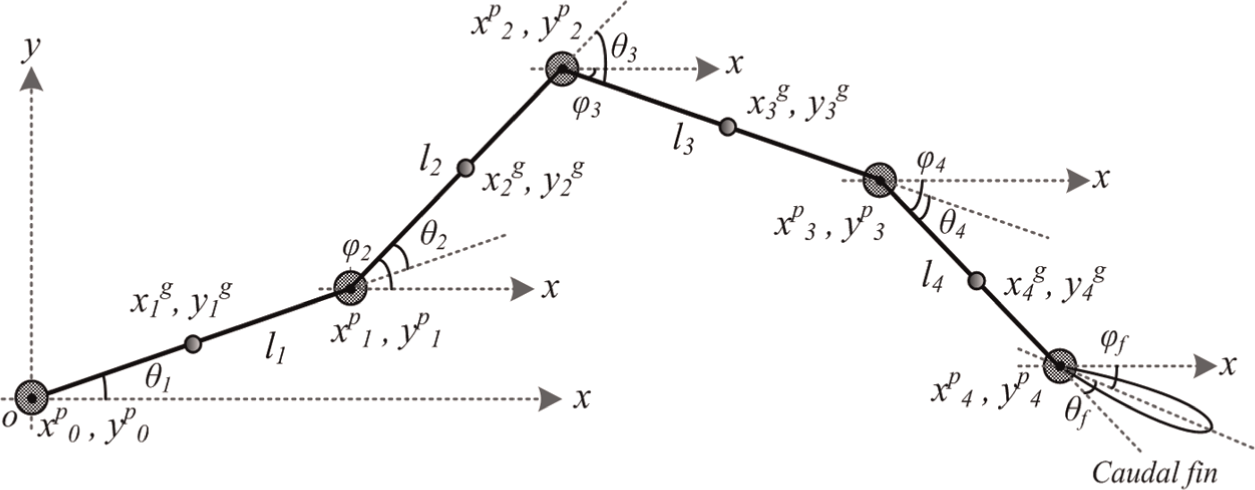
The flexible tail structure of the four-joint robotic fish.

Each angle between l_j₋₁ and l_j joints is represented by θ_j and φ_j is the orientation of the joint angle according to the horizontal x-axis for the i joint. Then, the relative angle between two joints is obtained by Equation (4):

θ_{j} = φ_{i} - θ_{j - 1}

(4)

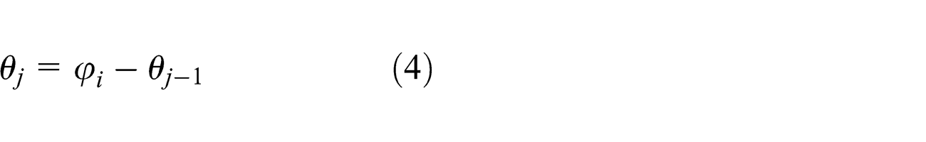
Figure 7 also shows the forces and moments acting on the each joint.

Figure 7.

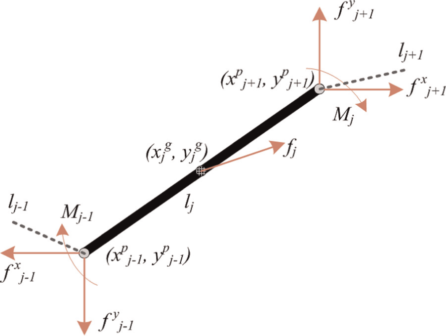
Free-body diagram: forces and moments acting on a link.

Here, the mass of each link and the moment of inertia related to the joints are represented by m_j, and I_j, respectively. Also, the centre of mass is indicated by (x^g_j y^g_j), while the forces and moments on each joint is represented by f_j and M_j. To present the kinematic model of the robotic fish, the assembly of flexible tail can be considered a robot manipulator with four variables and a fixed rotary joint. Thus, the expressions used to define a robot manipulator can be used to express the structure of the flexible tail. The D-H method is a standard representation to obtain the forward kinematic model of a robot manipulator (Kurfess, 2005; Bingül and Küçük, 2008; Watts et al., 2007). Firstly, the basic and local coordinate centres are principally placed on the joints for kinematic analysis. The basic coordinate centre is placed on the 0 point, while the local coordinate centres are placed on the rotational centres of joints. Any of the end joints of the fish robot can be taken as the base frame, because dynamic equations are the same in both ends of the joints. The joints rotate around the z-axis, which is perpendicular to the horizontal plane. In this way, the axis transformation required to build a D-H link parameter table is created as shown in Figure 8.

Figure 8.

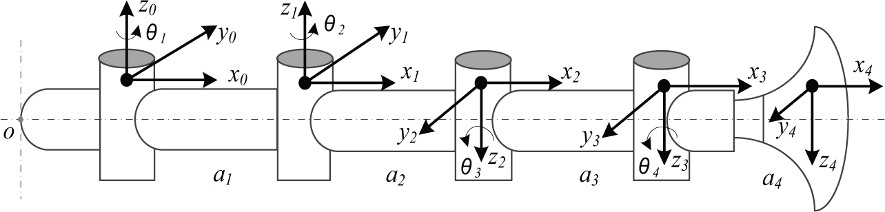
Placing the axis for forward kinematic.

Table 1 shows the D-H link conversion table for the four-joint mechanism of the robotic fish.

Table 1.

Denavit–Hartenberg (D-H) link parameter table.

Joint number	θ_j	a_j	α_j	Variables
1	θ ₁	a ₁	0	θ ₁
2	θ ₂	a ₂	π	θ ₂
3	θ ₃	a ₃	0	θ ₃
4	θ ₄	a ₄	0	θ ₄

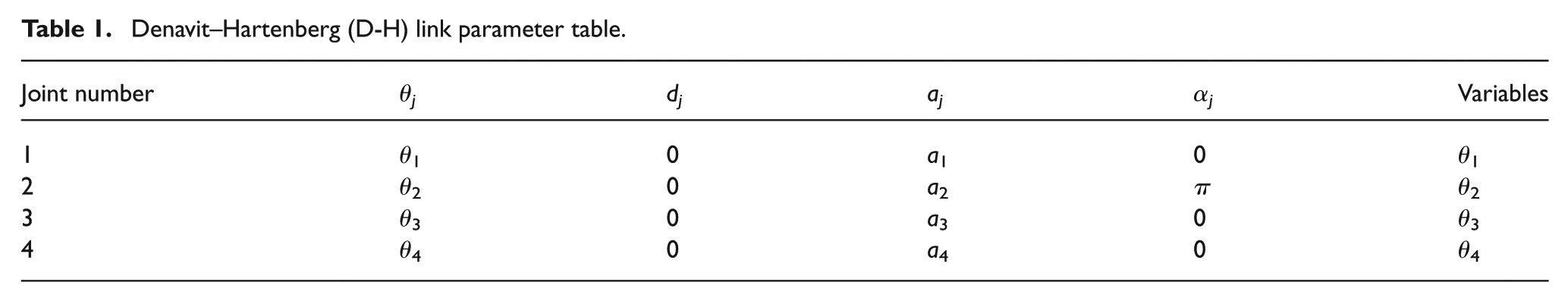
From the D-H conversion table, transformation matrices (A₁, A₂, …, A_N; N=4) are calculated for each joint. Using these matrices, the overall transformation matrix, which achieves the forward kinematic solution of the system, is determined as follows:

T^{body} = A_{1} . A_{2} . A_{3} . A_{4}

(5)

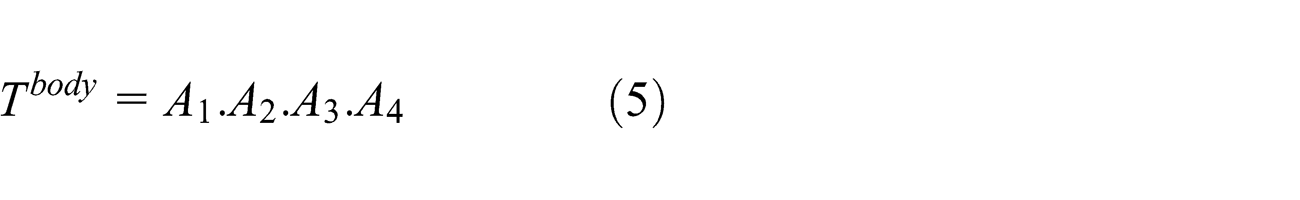
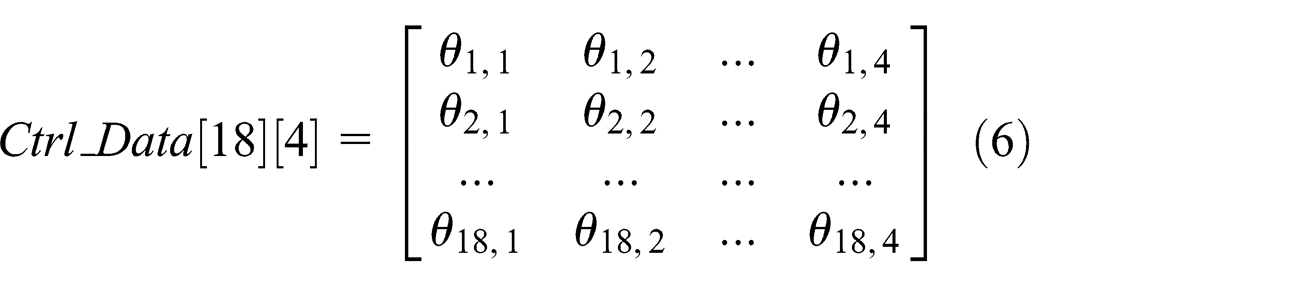
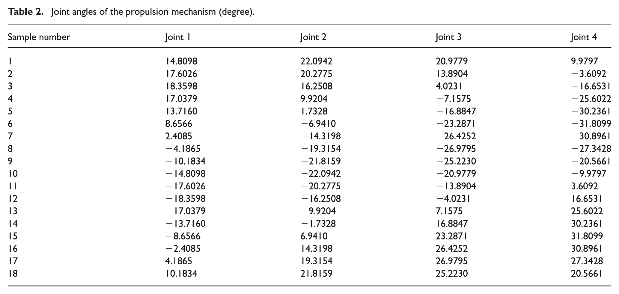
Using this transformation matrix, the position of the caudal fin is determined and the rotation angles of each driving element are obtained. Finally, these angles are applied to the robotic fish, such as illustrated in Equation (6). Thus, a 2-D rectangular matrix, a 18×4 look-up table, is obtained for the joint angle θ_ij and each angle is used for control data of the robotic fish.

Ctrl_Data [18] [4] = [\begin{matrix} θ_{1, 1} & θ_{1, 2} & . . . & θ_{1, 4} \\ θ_{2, 1} & θ_{2, 2} & . . . & θ_{2, 4} \\ . . . & . . . & . . . & . . . \\ θ_{18, 1} & θ_{18, 2} & . . . & θ_{18, 4} \end{matrix}]

(6)

The obtained joint angles of the robotic fish are given for one oscillation period in Table 2. Eventually, the robotic fish can swim like a real carangiform swimmer.

Table 2.

Joint angles of the propulsion mechanism (degree).

Sample number	Joint 1	Joint 2	Joint 3	Joint 4
1	14.8098	22.0942	20.9779	9.9797
2	17.6026	20.2775	13.8904	−3.6092
3	18.3598	16.2508	4.0231	−16.6531
4	17.0379	9.9204	−7.1575	−25.6022
5	13.7160	1.7328	−16.8847	−30.2361
6	8.6566	−6.9410	−23.2871	−31.8099
7	2.4085	−14.3198	−26.4252	−30.8961
8	−4.1865	−19.3154	−26.9795	−27.3428
9	−10.1834	−21.8159	−25.2230	−20.5661
10	−14.8098	−22.0942	−20.9779	−9.9797
11	−17.6026	−20.2775	−13.8904	3.6092
12	−18.3598	−16.2508	−4.0231	16.6531
13	−17.0379	−9.9204	7.1575	25.6022
14	−13.7160	−1.7328	16.8847	30.2361
15	−8.6566	6.9410	23.2871	31.8099
16	−2.4085	14.3198	26.4252	30.8961
17	4.1865	19.3154	26.9795	27.3428
18	10.1834	21.8159	25.2230	20.5661

Dynamic model of the robotic fish

To analyse the motion of the robotic fish, a dynamic model is required. Based on the biological structure of carangiform motion, the robotic fish is considered a typical serial robot manipulator and it can be modelled by the function of the Lagrange (L) approach (Zhou et al., 2008). The robotic fish swims in water autonomously and the motion of the links interacts with water. The kinematic and dynamic models are interrelated and Equation (3) describes the motion and depends on the motion laws of the links. The basic method for modelling a biomimetic robotic fish is to establish the L-function based on the structure of the four-joint mechanism. The generalized forces obtained from the L-function of the second kind are equal to the calculated forces from the hydrodynamics. Finally, partial differential equations are obtained and the motion of the robotic is solved and designed. For this approach, some assumptions can be given to simplify the system model (Zhou et al., 2008):

The body of robotic fish can be considered an N series of links together: N=4.

The robotic fish swims on still water and it is not affected by influence from the environment.

The motion of the robotic fish is modelled only in a 2-D plane, which is agreed as the most usable and representative.

The Lagrange approach is expressed by the total kinetics and potential energies of the system. The L-function can be created by the following general statement:

L (q, \overset{\cdot}{q}) = T (q, \overset{\cdot}{q}) - V (q)

(7)

\frac{d}{dt} (\frac{\partial L}{\partial {\overset{\cdot}{q}}_{i}}) - \frac{\partial L}{\partial q_{i}} + \frac{\partial F_{D}}{\partial {\overset{\cdot}{q}}_{i}} = τ_{i} i = 1, 2, . . ., N

(8)

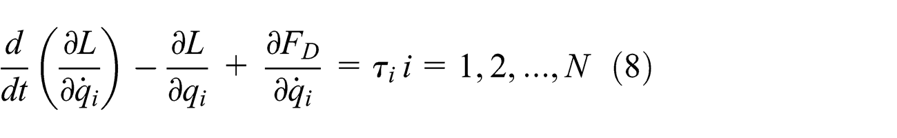
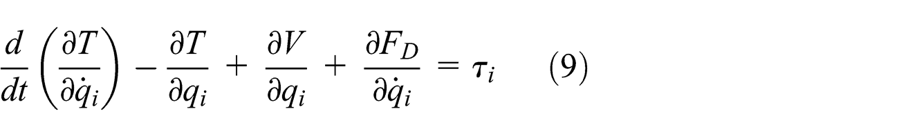
Here, T and V represent the total kinetics and potential energies of the system, respectively. F_D is external viscosity force acting on the system. q represents the joint angle while its first derivative represents the joint velocity. Also, τ_i represents the torque vector. If Equation (8) is clearly written again:

\frac{d}{dt} (\frac{\partial T}{\partial {\overset{\cdot}{q}}_{i}}) - \frac{\partial T}{\partial q_{i}} + \frac{\partial V}{\partial q_{i}} + \frac{\partial F_{D}}{\partial {\overset{\cdot}{q}}_{i}} = τ_{i}

(9)

The total kinetics energy is equal to the sum of the kinetics energy of each joint and it can be expressed by Equation (10):

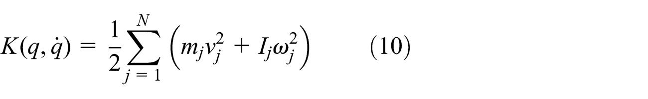
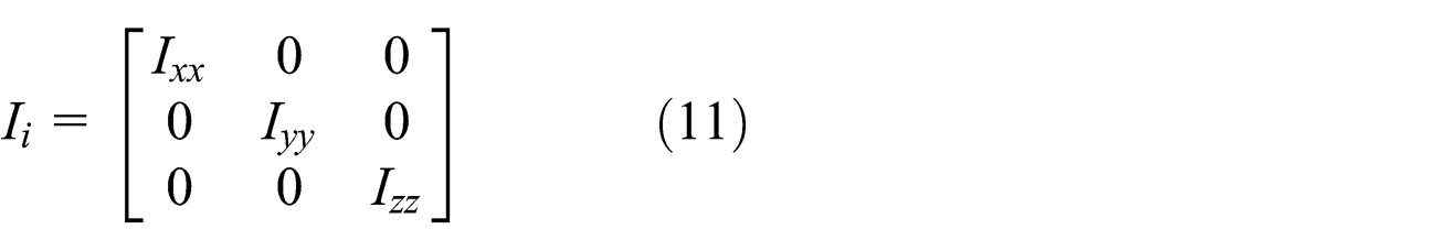
K (q, \overset{\cdot}{q}) = \frac{1}{2} \sum_{j = 1}^{N} (m_{j} v_{j}^{2} + I_{j} ω_{j}^{2})

(10)

Here, m_j represents the mass of the j joint, while I_j represents the moment of inertia of j joint. v_j and w_j represent the linear and angular velocities of the j joint, respectively. According to these descriptions, the moment of inertia of the j joint is defined as follows:

I_{i} = [\begin{matrix} I_{xx} & 0 & 0 \\ 0 & I_{yy} & 0 \\ 0 & 0 & I_{zz} \end{matrix}]

(11)

At the same time, the total potential energy expression is obtained as follows:

P (q) = \sum_{i = 1}^{n} m_{i} {gh}_{i}

(12)

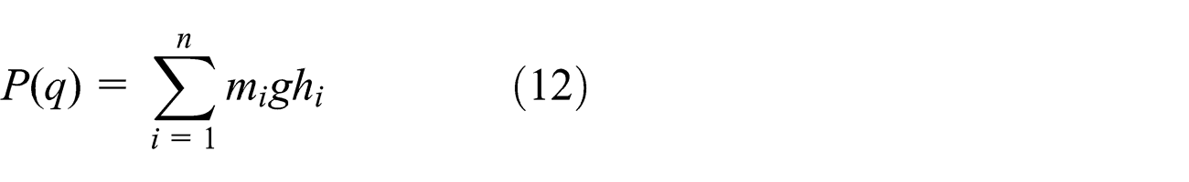
Here, g represents the gravitational acceleration. The total potential energy of the system is the z-axis direction for the designed robotic fish moving in the x–y plane. In this way, the acceleration of gravity occurs in the perpendicular direction to the x–y plane and it is a constant value. Considering the external forces acting on the system, if phrases representing in the kinetics and potential energies are written instead, the new equation is obtained as follows:

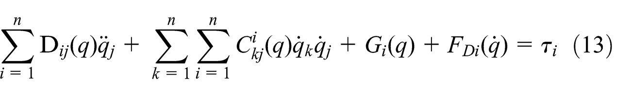
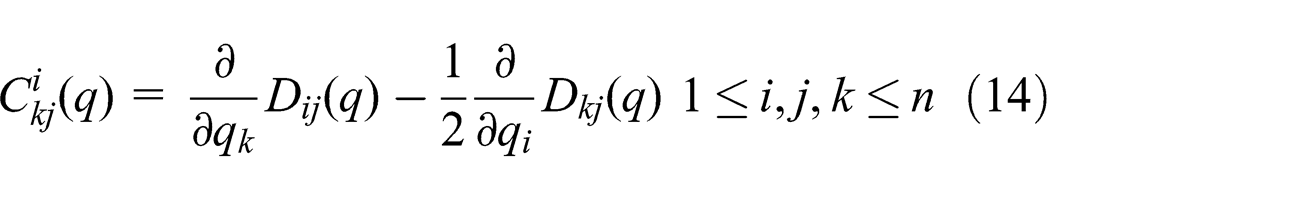
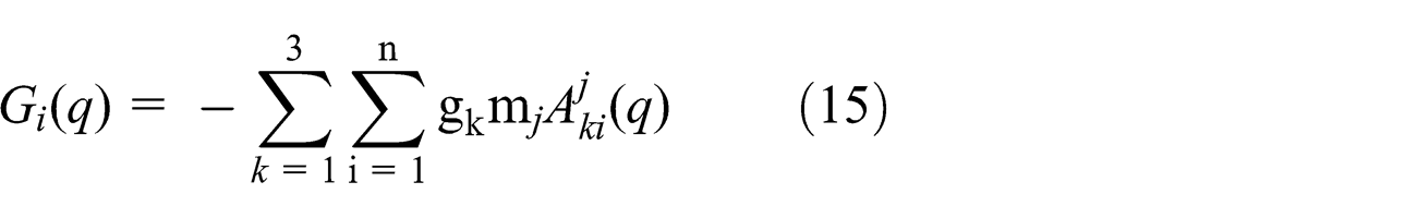
\sum_{i = 1}^{n} D_{ij} (q) {\overset{\cdot\cdot}{q}}_{j} + \sum_{k = 1}^{n} \sum_{i = 1}^{n} C_{kj}^{i} (q) {\overset{\cdot}{q}}_{k} {\overset{\cdot}{q}}_{j} + G_{i} (q) + F_{Di} (\overset{\cdot}{q}) = τ_{i}

(13)

Here, the mass matrix of joints is represented by D, the coriolis force matrix is represented by C and the matrix G represents the gravitational acceleration. Finally, F_D represents external forces acting on the system. The gravitational acceleration and coriolis matrix are obtained by Equations (14) and (15), respectively (Bingül and Küçük, 2008):

C_{kj}^{i} (q) = \frac{\partial}{\partial q_{k}} D_{ij} (q) - \frac{1}{2} \frac{\partial}{\partial q_{i}} D_{kj} (q) 1 \leq i, j, k \leq n

(14)

G_{i} (q) = - \sum_{k = 1}^{3} \sum_{i = 1}^{n} g_{k} m_{j} A_{ki}^{j} (q)

(15)

The viscosity force acting on the robot fish can be expressed as below:

F_{D} = \frac{1}{2} C_{D} ρ V^{2} S_{a}

(16)

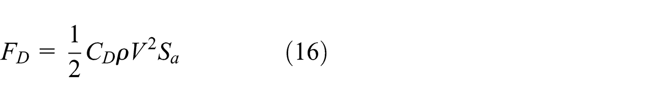
where C_D is the drag coefficient depended on the Reynolds number, ρ is the water density, V is the speed of the robotic fish and S_a is the surface area of water. As a result, the obtained dynamic model of the robotic fish is given in Equation (17):

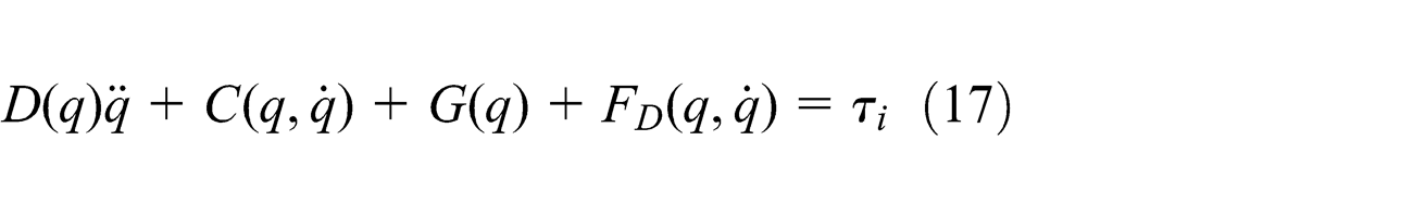
D (q) \overset{\cdot\cdot}{q} + C (q, \overset{\cdot}{q}) + G (q) + F_{D} (q, \overset{\cdot}{q}) = τ_{i}

(17)

Thus, the motion of the robotic fish is obtained as given in Equation (17). The dynamic model is established to perform the numerical solution of Lagrange’s equations for each joint and converted to the state-space model for linearization in the MATLAB/Simulink environment.

Simulation and experimental results

Based on the biological structure of carangiform motion, the multi-joint propulsion mechanism is considered a typical serial robot manipulator and the robotic fish is modelled by the function of the L approach. The obtained dynamic model from this approach is performed in MATLAB by numerical solution and converted to the state-space model to analyse and control each joint in MATLAB/Simulink environment. Consequently, carangiform motion is developed using joint angles and a biomimetic robotic fish model can be implemented.

The state feedback control can be considered one of the more modern control techniques and represents the system in terms of its input, output and the state variables related by first-order differential equations. This control method is usually used on position control applications in the robotics. Also, the state-space representation provides a compact way to analyse systems with multiple inputs and outputs (Akyuz et al., 2011; Honkakorpi et al., 2013; Jain et al., 2013). An open-loop state-space model of a system is represented by Equation (18):

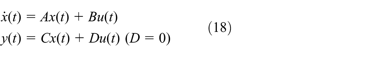
\begin{matrix} \overset{\cdot}{x} (t) = Ax (t) + Bu (t) \\ y (t) = Cx (t) + Du (t) (D = 0) \end{matrix}

(18)

where x(t) is the state variables vector, y(t) is the output vector and u(t) is the input vector. The matrices A, B, C and D are the state, input, output and zero matrices, respectively. Also, size of A, B, C and D matrices are (8×8), (8×4), (4×8) and (4×4) in the simulation results.

The state-space model has more advantages in that it gives information about both state and input–output variables (Jain et al., 2013). In the simulation results, the state-space model is developed and PID-based state feedback control is performed using the dynamic model of the four-joint robotic fish. The block scheme of the PID-based state feedback control model is shown in Figure 9.

Figure 9.

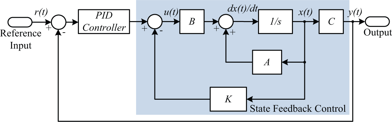
The state-space model of the robotic fish.

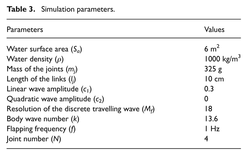
Here, moments of the joints (M_j) are input variable of the closed-loop control system and joint angles (Θ_j) are the output variables. Using state-space matrices of the system, the K gain value is calculated and state-space design is performed. Thus, the robotic fish model is stabilized and controlled with a conventional PID controller for each joint. In the simulation results, parameters of the PID K_p, K_i and K_D are obtained using a classic trial-and-error method. The parameters used in the simulation studies are given in Table 3.

Table 3.

Simulation parameters.

Parameters	Values
Water surface area (S_a)	6 m²
Water density (ρ)	1000 kg/m³
Mass of the joints (m_j)	325 g
Length of the links (l_j)	10 cm
Linear wave amplitude (c₁)	0.3
Quadratic wave amplitude (c₂)	0
Resolution of the discrete travelling wave (M_f)	18
Body wave number (k)	13.6
Flapping frequency (f)	1 Hz
Joint number (N)	4

Simulations of the dynamic behaviour

Simulation of the state feedback control is realized in the MATLAB/Simulink environment. The joint angles obtained from the kinematic model of the robotic fish are applied to the state feedback model to mimic autonomous swimming of carangiform motion. As shown in Figure 10, the joint angles are given for forward swimming. A good closed-loop control performance is obtained in the simulation results and closed-loop output signals are given in Figure 11.

Figure 10.

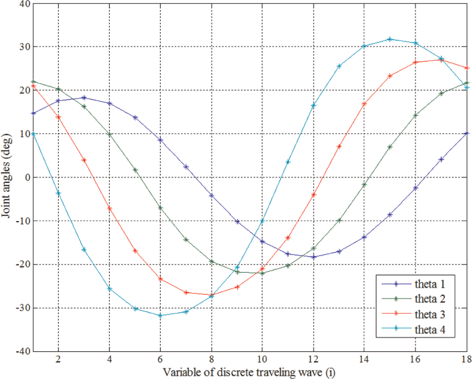
The joint angles for forward swimming at f=1 Hz flapping frequency.

Figure 11.

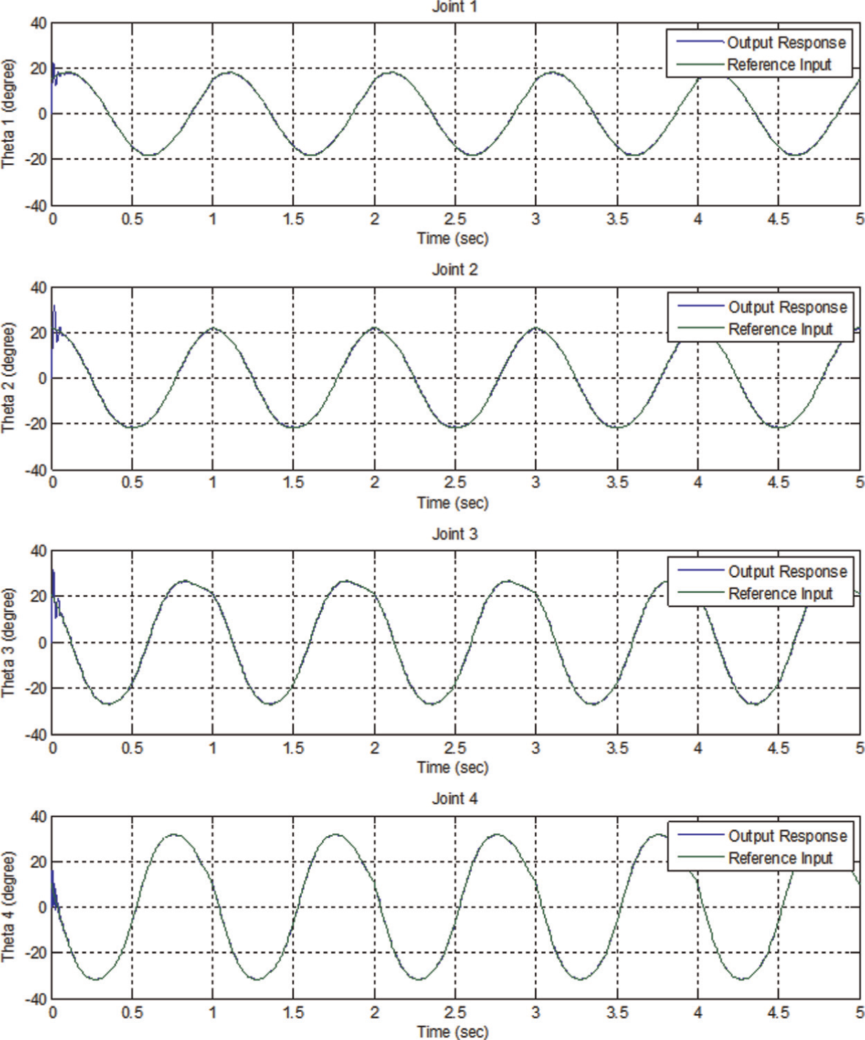
Closed-loop response of the joint angles.

Error signals of the closed-loop control system are given as seen in Figure 12.

Figure 12.

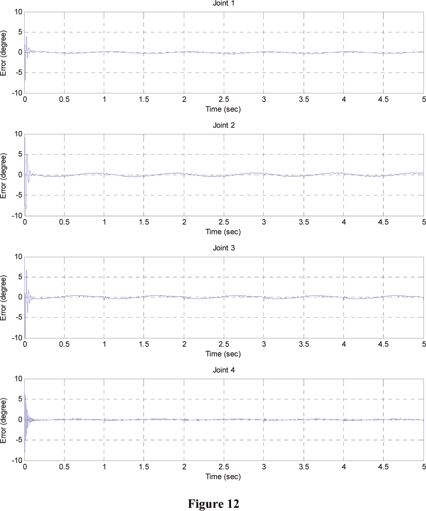
Error signals of the joint angles.

Furthermore, a solid model of the robotic fish prototype is drawn in SolidWorks. This model is transferred to the MATLAB/Simmechanics environment and motion of the controlled system is simulated using joint angles. The sequences of obtained results from the robotic fish simulation are given in Figure 13.

Figure 13.

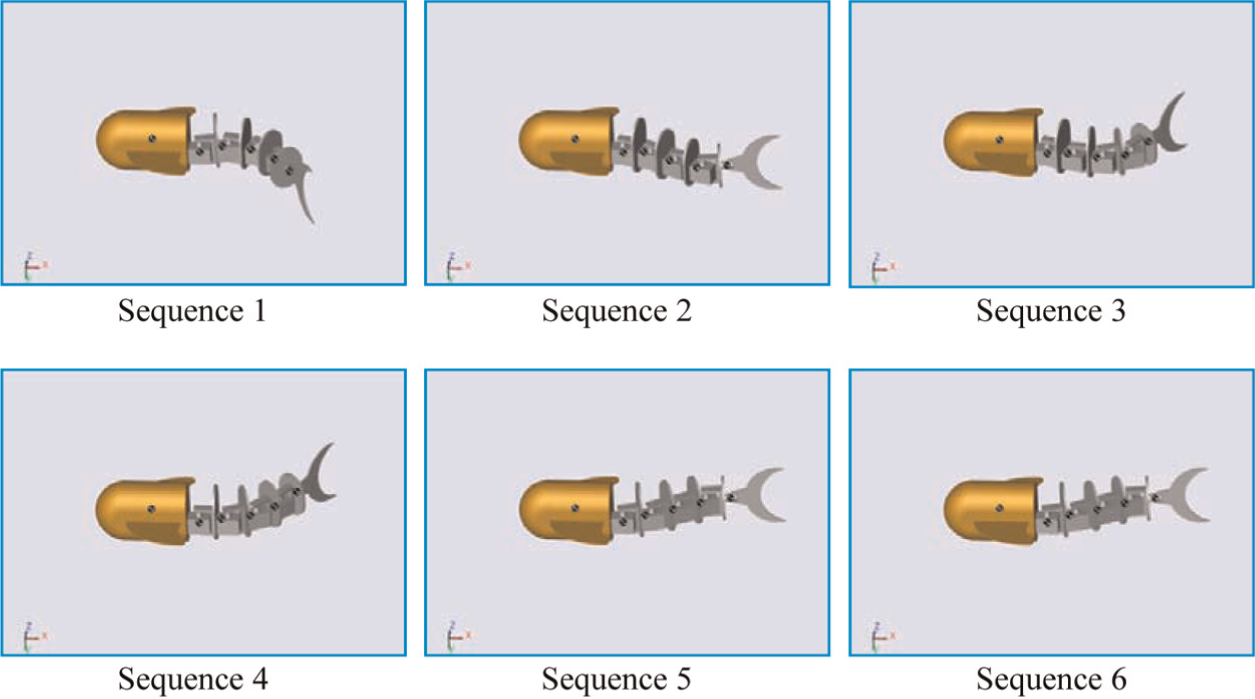
Visual simulations of the carangiform motion for forward swimming.

As shown in Figure 11, joint angles are controlled according to the desired angles and provided carangiform motion in the simulation. Figure 12 shows that the error signals of the closed-loop system are appropriately minimized for the desired angles. Also, motion performance of the robotic fish is tested and the desired motion capability is obtained using a solid model.

Experiments of the robotic fish

Based on the fundamental biological structure, a remote-controlled, multi-joint and autonomous-swimming biomimetic robotic fish prototype is implemented (Korkmaz, 2012). Figure 14(a) shows the mechanical configuration of the robotic fish and the experimental photo image from the robotic fish prototype is given in Figure 14(b).

Figure 14.

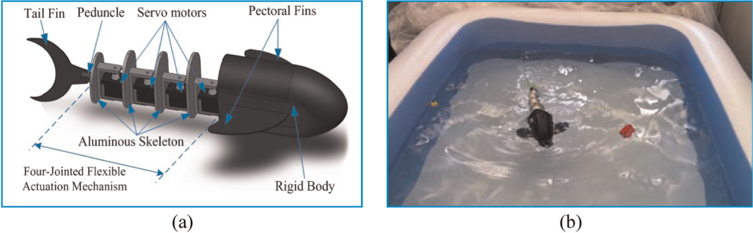
The implementation of a biomimetic robotic fish: (a) solid model of the robotic fish; (b) prototype of the robotic fish in the pool.

An anterior rigid body and a posterior flexible tail, which includes four-joint propulsion mechanism, are used in this model. The flexible tail consists of four DC servo motors. The robotic fish has two swimming modes: autonomous and remote-controlled swimming. Firstly, it can swim like a real carangiform swimmer in the water without a remote controller. When the robotic fish comes up against an obstacle, it can perceive the obstacles with its IR sensors and it can sense the obstacles within a range of 40 cm. This behaviour is for getting away from other fish or obstacles. A significant feature of this behaviour is that the robotic fish can change its direction autonomously. Secondly, it can be controlled by a remote controller. Thus, the robotic fish can be turned to the desired direction and the pectoral fins can be controlled. Moreover, if there is an obstacle in the desired direction, the robotic fish does not turn towards in that direction until it exceeds the obstacle. In addition, a wireless camera is placed in the head of fish to take underwater image information to a personal computer. In this way, the underwater image information can be evaluated (Korkmaz et al., 2012).

The flexible propulsion mechanism is the kinetic part of the robotic fish and it determines the capability for carangiform motion. To achieve smooth motions like a real fish, the robotic fish should have as many joints as possible, but due to design limitations of driving elements and in order to design a compact prototype, a four-joint mechanism is used. Thus, a simpler design and high applicability model is obtained.

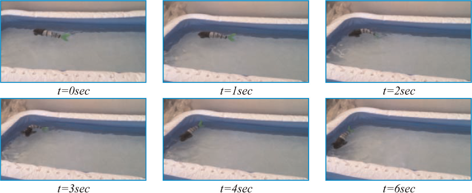
To realize the proposed design, experimental studies are performed in a pool with dimensions of 305×183×56 cm (length×width×depth). A CCD camera is used to identify the swimming information and motion status of the robotic fish. The camera is connected to the personal computer and the captured image information can be achieved in real time. The speed of the robotic fish is tuned by modulating the flapping frequency (f) of the multi-joint mechanism, generating different body wave amplitude values (c₁ and c₂) and changing the length of the flexible tail mechanism (l). Moreover, the position of the robotic fish is adjusted by different joint deflections. Forward swimming and turning motion at different times in the pool are shown in Figures 15 and 16, respectively.

Figure 15.

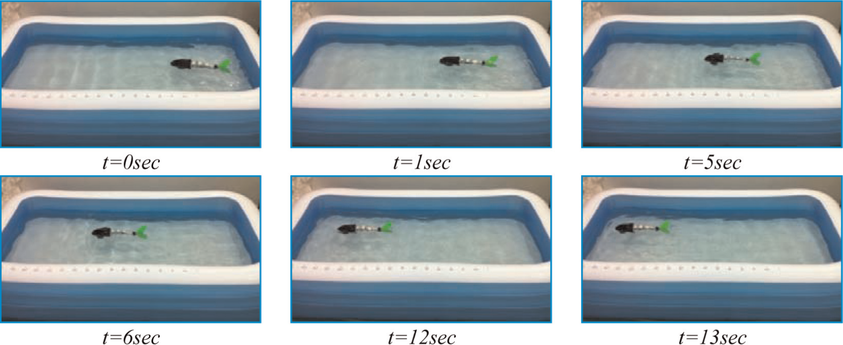
The snapshot sequence: swimming of the robotic fish for forward swimming in the pool.

Figure 16.

The snapshot sequence: turning motion of the robotic fish in the pool.

In the experimental studies, the obtained joint angles from the simulation results are used. Figure 15 shows that the robotic fish mimics real carangiform motion for forward-swimming ability. If the robotic fish comes up against an obstacle it can perceive the obstacles with its IR sensors and it can sense the obstacles within a range of 40 cm. Comparing experimental studies with simulation results, a carangiform motion for autonomous swimming is developed.

Conclusions

In this paper, an overall design approach for a multi-joint propulsion model for carangiform motion is given and a dynamic model of the carangiform-type biomimetic robotic fish is obtained using the Lagrange approach. The designed robotic fish consists of two parts: an anterior rigid body and a flexible tail, which modelled as a four-joint propulsion mechanism. The flexible tail mechanism is actuated by four DC servo motors. Using an established dynamic model of the robotic fish, state feedback control is performed in the MATLAB/Simulink environment. To stabilize the dynamic model, the K gain value is calculated and state-space design is performed. Thus, the robotic fish model is controlled with a conventional PID controller for each joint. In the simulation studies, joint angles are derived and applied to the dynamic model to mimic the forward-swimming motion of the carangiform swimmers. The simulation results indicate that real carangiform motion is achieved using this model. Moreover, a solid model of the robotic fish prototype is drawn in SolidWorks and transferred to the MATLAB/Simmechanics environment, and the motion of the controlled system is simulated using joint angles. Finally, comparing experimental studies with simulation results shows that carangiform motion for autonomous swimming is developed using controlled joint angles. However, experimental studies show that the mechanical structure and skin material of the robotic fish should be improved in order to achieve efficient and robust swimming.

Future research will focus on navigating in a 3-D workspace to verify the model fully, and the robotic fish prototype will be improved to obtain more efficient swimming motion.

Footnotes

Acknowledgements

The authors would like to thanks for financial support of Fırat University.

Conflict of interest

The authors declare that there is no conflict of interest.

Funding

This work was funded by research grant from Fırat University Scientific Research Projects Unit (FUBAP-2095).

References

Akyuz

Yolacan

Ertunc

. (2011) PID and state feedback control of a single-link flexible joint robot manipulator. IEEE International Conference on Mechatronics (ICM), Istanbul, pp. 409–414.

Bingül

Küçük

(2008) Dynamics of Robot and Control. Istanbul: Birsen Press.

Chen

Shatara

Tan

(2009) Modeling of biomimetic robotic fish propelled by an ionic polymer-metal composite caudal fin. IEEE/ASME Transactions on Mechatronics 15: 1–12.

Hirata

(1999) Design and manufacturing of a small fish robot. Processing of Japan Society for Design Engineering 99: 29–32.

Honkakorpi

Vihonen

Mattila

(2013) MEMS-based state feedback control of multi-body hydraulic manipulator. IEEE/RSJ International Conference on Intelligent Robots and Systems (IROS), Tokyo, pp. 4419–4425.

(2006) Biologically inspired design of autonomous robotic fish at Essex, Proceedings of the IEEE SMC UK-RI Chapter Conference on Advances in Cybernetic Systems, Sheffield, pp. 1–8.

Liu

Dukes

. (2006) Design of 3D swim patterns for autonomous robotic fish. IEEE/RSJ International Conference on Intelligent Robots and Systems, Beijing, pp. 2406–2411.

Jain

Sugumaran

Wadoo

(2013) Establishing a cost effective embedded control and robotics engineering program: observer based state feedback control using LEGOs. IEEE Integrated STEM Education Conference (ISEC), Princeton, NJ, pp. 1–6.

Korkmaz

(2012) Design and implementation of a remote-controlled robotic fish. Master thesis. Fırat University Graduate School of Natural and Applied Sciences.

10.

Korkmaz

Ozmen Koca

Akpolat

(2011) Robust forward speed control of a robotic fish. 6th International Advanced Technologies Symposium, Elazig, Turkey, pp. 33–38.

11.

Korkmaz

Budak

Bal

. (2012) Modeling and implementation of a biomimetic robotic fish. International Symposium on Power Electronics, Electrical Drives, Automation and Motion, SPEEDAM12, Sorrento, Italy, pp. 1187–1192.

12.

Kurfess

(2005) Robotics and Automation Handbook. Boca Raton, FL: CRC Press.

13.

Lighthill

(1960) Note on the swimming of slender fish. Journal of Fluid Mechanics 9: 305–317.

14.

Liu

(2004) A 3D simulator for autonomous robotic fish. International Journal of Automation and Computing 1: 42–50.

15.

Liu

Dukes

Knight

. (2004) Development of fish-like swimming behaviours for an autonomous robotic fish. Proceedings of Control, University of Bath, pp. 6–9.

16.

Morgansen

Duidam

Mason

. (2001) Nonlinear control methods for planar carangiform robot fish locomotion. ICRA 1, Proceedings of the 2001 IEEE International Conference on Robotics and Automation1, pp. 427–434.

17.

Qiu

Liu

(2007) A methodology of modelling fish-like swim patterns for robotic fish. Proceedings of IEEE 2007 International Conference on Mechatronics and Automation, Harbin, China, pp. 1316–1321.

18.

Sfakiotakis

Lane

Davies

JBC

(1999) Review of fish swimming modes for aquatic locomotion. IEEE Journal of Ocean Engineering 24: 237–252.

19.

Tan

. (2014) Implementing flexible and fast turning maneuvers of a multijoint robotic fish. IEEE/ASME Transaction on Mechatronics 19: 329–338.

20.

Tong

(2000) Propulsive mechanism of Fsh's Undulatory Motion. Mechanic in Engineering 22(3): 69–74.

21.

Triantafyllou

(1995) An efficient swimming machine. Scientific American 272: 64–70.

22.

Vepa

(2009) Biomimetic Robotics Mechanisms and Control. New York: Cambridge University Press.

23.

Watts

McGookin

Macauley

(2007) Modelling and control of a biomimetic underwater vehicle with a tendon drive propulsion system. Oceans 2007–Europe, Aberdeen, pp. 1–6.

24.

Wen

Wang

. (2012) Novel method for the modeling and control investigation of efficient swimming for robotic fish. IEEE Transactions on Industrial Electronics 59: 3176–3188.

25.

Guo

. (2008) Design and realization of a remote control centimeter-scale robotic fish. AIM 2008, IEEE/ASME International Conference on Advanced Intelligent Mechatronics, Xian, China, pp. 25–30.

26.

Wang

Tan

(2003) Design of a free-swimming biomimetic robot fish. IEEE/ASME International Conference on Advanced Intelligent Mechatronics, Port Island, Kobe, Japan, pp. 95–100.

27.

Tan

Wang

. (2004) Development of a biomimetic robotic fish and its control algorithm. IEEE Transactions on Systems, Man, and Cybernetics – Part B: Cybernetics 34: 798–1810.

28.

Wang

Tan

(2005) A simplified propulsive model of biomimetic robot fish and its realization. Robotica 23: 101–107.

29.

Liu

Wang

(2006) Dynamic modeling of robotic fish using Schiehien’s method. IEEE International Conference on Robotics and Biomimetics, ROBIO’06, Kunming, China, pp. 457–462.

30.

Liu

Tan

(2008) Three-dimensional dynamic modeling of robotic fish: simulations and experiments. Transactions of the Institute of Measurement and Control 30: 239–258.

31.

Zhang

Zhao

. (2007) Development and depth control of biomimetic robotic fish. Proceedings of the 2007 IEEE/RSJ International Conference on Intelligent Robots and Systems, San Diego, CA, pp. 3560–3565.

32.

Zhang

Yamashita

Gondo

. (2008) Electrostatically actuated robotic fish: design and control for high-mobility open-loop swimming. IEEE Transactions on Robotics 24: 118–129.

33.

Zhou

Cao

Wang

. (2008) The dynamic analysis of the backward swimming mode for biomimetic carangiform robotic fish. IEEE/RSJ International Conference on Intelligent Robots and Systems, Nice, France, pp. 3072–3076.

34.

Zhou

Cao

Wang

. (2010) A Marsupial Robotic Fish Team: Design, Motion and Cooperation. Berlin: Science China Press and Springer-Verlag, 53, pp. 2896–2904.