
Abstract
The purpose of this paper is to present an original method for system monitoring with Bayesian networks. Our proposal is to associate a data-driven method to another model-based under a common tool. The two methods are first modeled under a Bayesian network (conditional Gaussian network), and then combined to evaluate the system state. In the proposed framework the residuals and measures coexist under a probabilistic framework. This approach is tested on a simulation of a water heater process under some various circumstances and shows better results than the two methods used alone.
Keywords
Introduction
The goal of businesses and industries to optimize gain/loss and the growing demand for increased product quality have immensely contributed to the development and the imperative use of monitoring methods (fault detection and isolation (FDI); fault detection and diagnosis (FDD)) among other means of operating safety. These methods are used to describe and explain, at each instant, the system state. They try to detect early faulty situations and provide their diagnosis when they occur.
Many (FDD, FDI) methods have emerged in the recent years (Chiang et al., 2001; Ding, 2011, 2008; Isermann, 2006; Qin, 2006). Among them, we can distinguish model-based methods and data-driven methods. Model-based methods (Ding, 2008; Frank et al., 2000; Gertler, 1991; Isermann, 2006; Patton et al., 1995) use prior knowledge explaining the system dynamics. This knowledge corresponds to a specific set of physical equations (e.g. quantitative model) representing the dependencies that may exist between system variables. It contributes to residuals generation (e.g. the difference between the measures taken on the system and their estimation). Once residuals are generated, they are immediately evaluated in order to describe the system operating state. In contrast, data-driven methods (Qin, 2006; Venkatasubramanian et al., 2003; Yin et al., 2012) use only system measures (e.g. sensors) taken at different times (historical data).
However, each of these monitoring methods has its advantages and drawbacks (Yew and Rajagopalan, 2010). The current majority strongly depend on the system nature and domain, and the quality, quantity and type of information available. Thus, many researchers (Chiang et al., 2001; Ding et al., 2009; Venkatasubramanian et al., 2003) suggest that the creation of a single framework using these two kind of methods, would allow a better system state description. Indeed, it seems clear that the data-driven methods capability to manage a significant number of data associated with the model-based methods ability to describe accurately the system dynamic behavior and provide physical understanding, could improve the system monitoring task. In the FDI–FDD literature, the major contributions generally focus on the development or improvement of one of both methods and, as far as we know this research field still unexplored, even if we can find some work describing the association attempts of these two types of methods (Ghosh et al., 2011; Luo et al., 2010; Schubert et al., 2011).
An unified scheme that integrates model-based and data-driven methods is proposed in Schubert et al. (2011). The authors combine subspace model identification (SMI) and univariate/multivariate statistical control methods with inputs reconstruction method and banks of unknown input observer (UIO). Luo et al. (2010) proposed a hybrid approach using parity equations and a nonlinear observer to generate residuals. Once the residuals generated, statistical tests are used to detect and isolate, with the aid of SVM (support vector machine), the different antilock braking system (ABS) faults. In Ghosh et al. (2011), a similar approach to those combining multiple classifiers (mixture of experts) in pattern recognition is used. Many decision fusion strategies (utility-based and evidence-based decision fusion strategies) of numerous fault detection and identification methods have been studied. For example, to monitor a laboratory distillation column, they use four heterogeneous methods: a model-based method (an extended Kalman filter) and three data-driven methods (SOM (self-organized map), ANN (artificial neural network) and PCA (principal component analysis)), where the output of each method corresponds to an assignment to a fault class.
The proposals mentioned above, despite the fact that they are attractive for the combination of data-driven and model-based methods, do not consider or address a particular problem which is the lack of data (e.g. some data are missing or insufficiently represented) and/or an approximation of the system model (e.g. unavailability of an accurate model). Moreover, instead of combining methods from a different nature and use different FDI–FDD tools to improve the decision making, it could be interesting to use a single tool associating and integrating data-driven and model-based methods. An attractive approach can be the use of Bayesian networks (BNs). They offer a probabilistic/statistical framework able to reason under uncertain knowledge and integrate information from different sources, in a natural way. In this paper, we propose a probabilistic FDI–FDD framework based on conditional Gaussian networks (CGNs), a particular class of BNs, able to use simultaneously the different information available on the system.
The paper is structured as follows: in Section 2 we introduce BNs, followed by a short description of some data-driven and model-based methods and their links to the BNs in Section 3; Section 4 describes the proposed monitoring methodology; the results of the proposed method tested on a heater water process under different conditions are outlined in Section 5; finally, the conclusions are described in the last section.
Bayesian networks
Definition
A BN is a probabilistic directed acyclic graph (Jensen, 1996) and it can be defined formally as:
a directed acyclic graph
a finite probabilistic space (Ω,
a set of random variables associated with the nodes of the graph
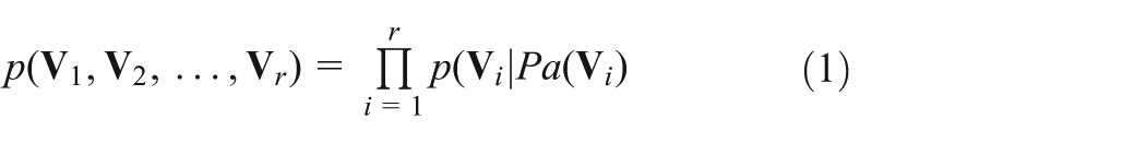
where Pa(
Conditional Gaussian networks
CGNs are a particular form of Bayesian networks. Each node in the network represents a random variable that could be discrete or Gaussian (univariate/multivariate). Arcs may exist between nodes from same or different nature (discrete or Gaussian). However, to ensure availability of exact inference (see (Lauritzen, 2001)), discrete variables are not allowed to have continuous parents. So, each discrete node given its parents, follows a multinomial distribution, generally outlined under a conditional probability table (CPT).
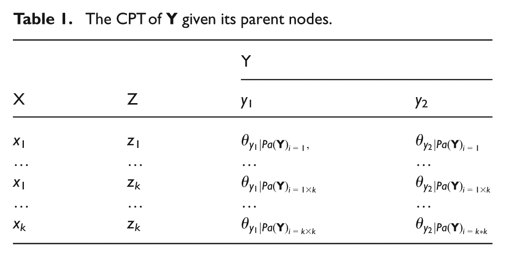
Consider a discrete node
The CPT of
Concerning the Gaussian nodes, they are allowed, unlike discrete nodes, to have Gaussian nodes as parents. Thus, we can distinguish two types of nodes. First, the Gaussian linear node
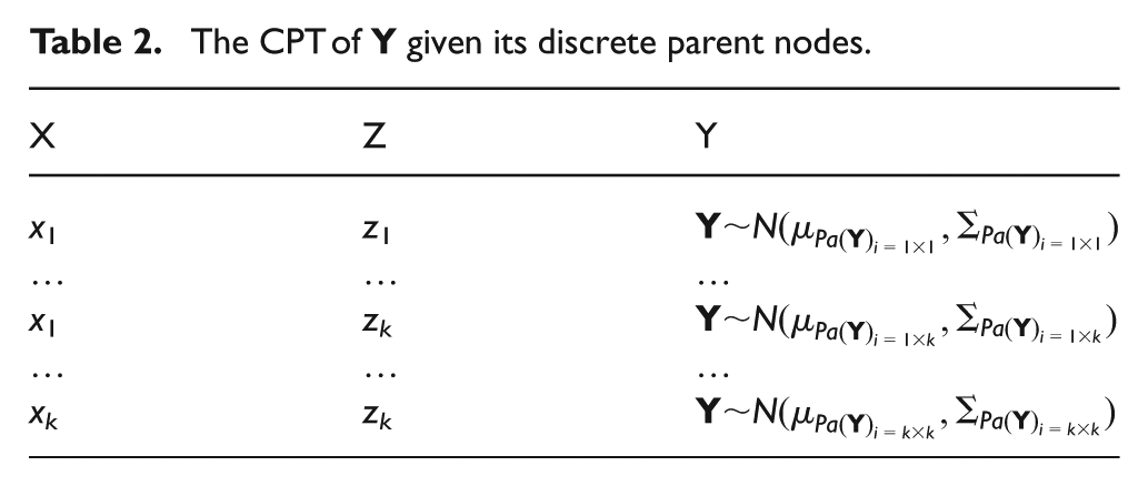
The second node is a Gaussian node with only discrete parents. Consider a Gaussian node
The CPT of
Several CGNs could be used to solve classification problems. One of them is the naive Bayesian network (NBN; see Figure 1). It assumes that the variables, child nodes of the decision discrete root node, are conditionally independent (the Gaussian nodes in the graph (circle form) are not connected). Another network is the condensed semi-naive Bayesian network (CSNBN; see Figure 1). It provide a simple structure that takes into account correlation that may exist under a group of variables (e.g. a single joint variable
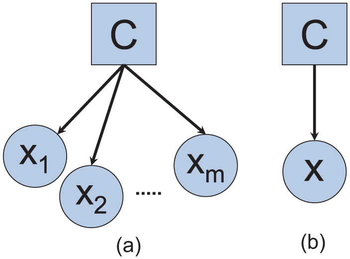
Bayesian network classifiers: (a) NBN and (b) CSNBN.
Fault detection and diagnosis
Fault detection and diagnosis are two phases that are usually associated. The first seeks to confirm at any moment whether the system is still in control (IC). Once a change is confirmed (the system is out of control (OC)), diagnosis procedures try to explain it, in order to make a decision about the system future (adjusting settings, maintenance, closure, etc.). The fault diagnosis phase can be defined in different ways (Chiang et al., 2001) depending on the type of the employed method and its description level.
Data-driven methods
FDD methods using system data (temporary or not) are called data-driven methods. Their effectiveness depends heavily on the quality and quantity of the data used. These last decades, several data-driven methods have been developed or enhanced. They correspond generally to rigorous statistical developments of the collected data. Almost all of them take into account correlation that may exist between the system variables and use multivariate statistical test to detect a change in the system. Among multivariate statistical tests, the most common in the literature are based on the T2 statistic (see (2), where x is an observation of a multivariate variable

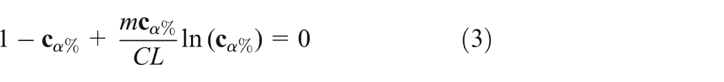
Once this statistic is calculated, the obtained scalar is analyzed with respect to a given false alarm rate. This is done by checking the obtained scalar membership over an interval (representing the system normal operation) bounded by an upper control limit (CL, very often it is chosen equal to
The T2 statistic can be modeled under a binary CSNBN classifier discriminating between the classes IC and OC. This BN (see Figure 2) consists of a multivariate Gaussian node
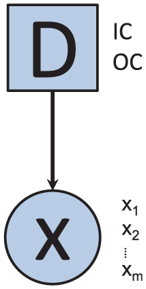
The statistical T2 under a CGN.
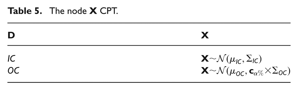
The nominal operating class IC is characterized by a mean μIC and a variance Σ
IC
, where the other alternative class OC is assumed expressing more variability through a coefficient
where m is the number of the system variables.
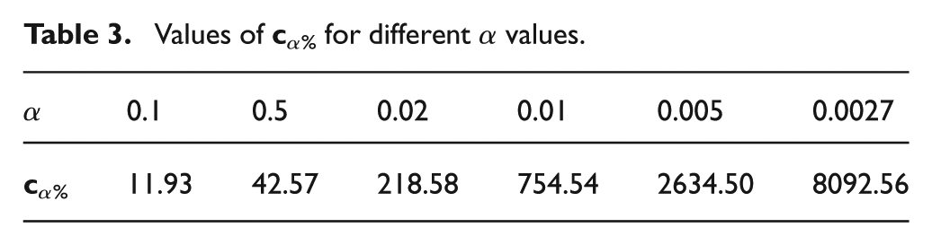
The demonstration of the computation of
Values of
The CPTs of the both nodes,
The node D CPT
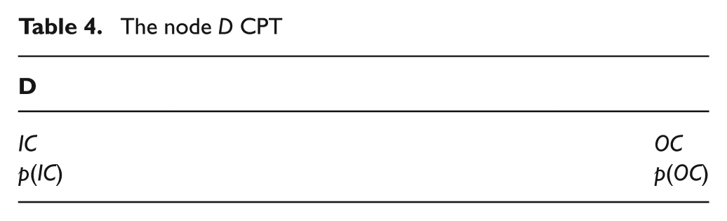
The node
For a given observation x of
Model-based methods
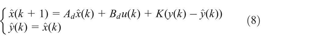
In the presence of an analytical system representation, model-based methods can be used. These methods calculate the difference between the measures taken on the system and their estimation. This difference is called residuals
The residuals, once generated, are immediately evaluated, very often independently of each others. The result of their evaluation is named symptoms
These tests can be also used to isolate a fault once detected. In this paper, we are interested in the well-known structured residuals approach (Gertler and Singer, 1990), where the residuals are generated so that they are sensitive only to certain faults. In order to made a decision, symptoms are compared (e.g. by a logic test) to each column of the incidence matrix (see Table 6). This matrix, for a given system, reflects its residuals sensitivity (
Incidence matrix example.
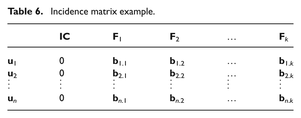
The incidence matrix can be modeled under a directed acyclic graph with discrete nodes able to make a decision given the observed symptoms, where faults are considered as the causes of the residuals deviation. Better yet, using a CGN as that given in Figure 3, we are able to model conjointly the residuals evaluation (based on the statistic T2) and the decision making (diagnosis based on the incidence matrix) as proposed by Verron et al. (2009).
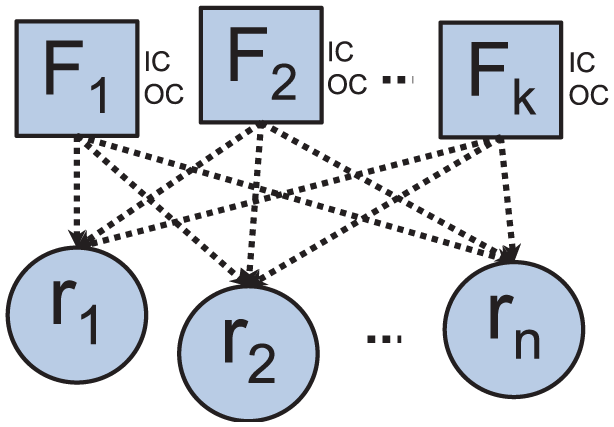
An incidence matrix on a CGN.
Proposed method
In this section, under a same tool, a CGN, a data-driven method and another model-based are proposed and associated to make better decisions.
CGN for data-driven monitoring
As a data-driven method, we propose to use a CGN, more precisely a CSNBN classifier, to discriminate between faults and the state IC (fault-free state H0). The proposed network (see Figure 4) is consisting of a discrete node
CGN for data-driven monitoring.
Once the network updated, given a new observation, a decision is made and the state with the maximum posterior probability is taken. Following this rule, the proposed network reflects a discriminant analysis:
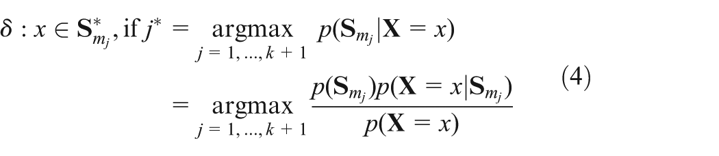
where
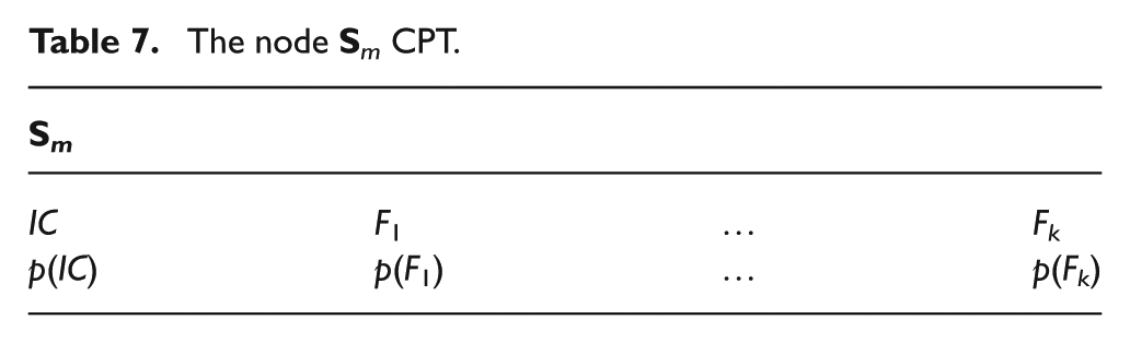
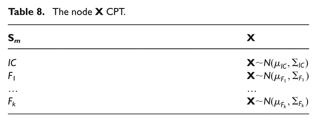
Using the proposed data-driven network, we are able to decide at each instant as to which operating state the system belongs. The probabilities tables corresponding to each node are shown in Tables 7 and 8.
The node
The node
CGN for model-based monitoring
In order to assist the CGN given above, another diagnosis strategy is considered. Instead using the available system data, it is based on the available system model, more exactly on the generated residuals and the defined incidence matrix. The proposed CGN as a model-based method is made of: a discrete node
However, as the normal operating state IC is associated to a null characteristic vector [0,…,0]T in the incidence matrix (see Table 6), the node

CGN for model-based monitoring.
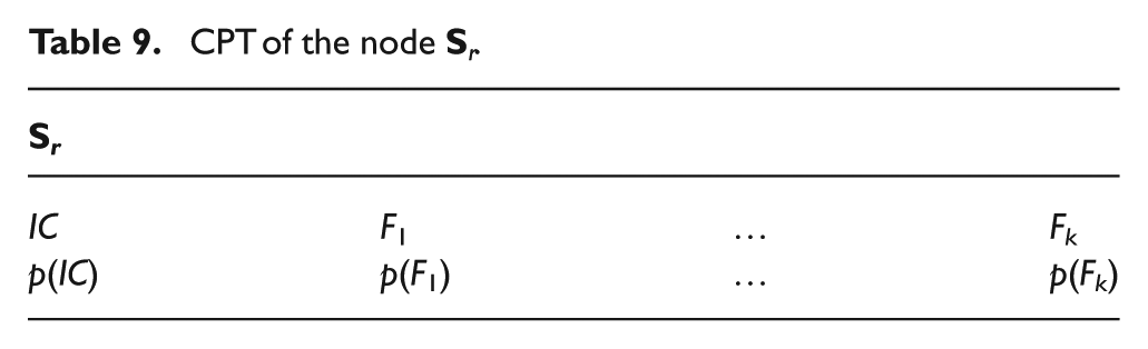
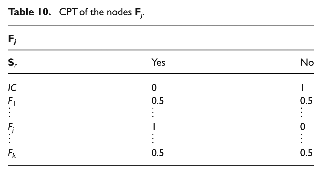
The CPTs of the node
CPT of the node
CPT of the nodes
Probabilistic framework for system monitoring
In order to make a decision about the system state and use the maximum amount of information available on the system, we suggest a probabilistic framework handling the system observed variables and generated residuals. To do so, a new discrete node
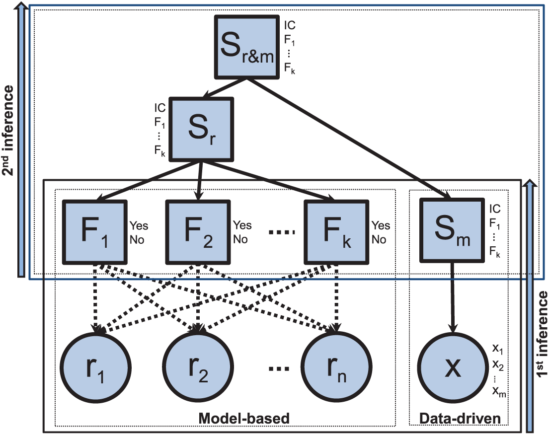
The proposed network.
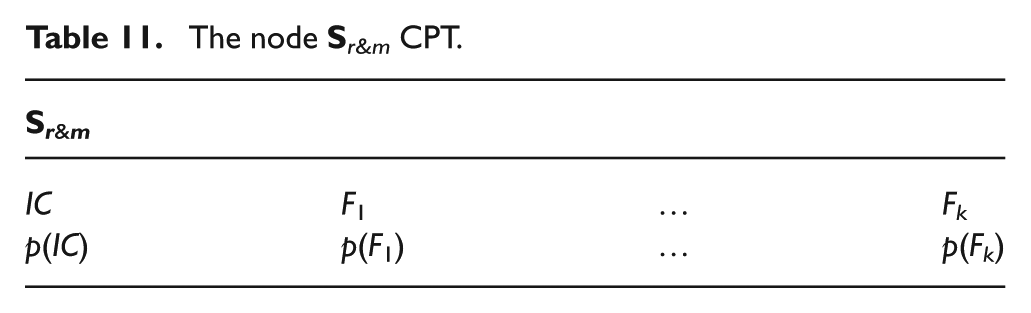
The CPT of the node
The node
The posterior probability of each state j of the node
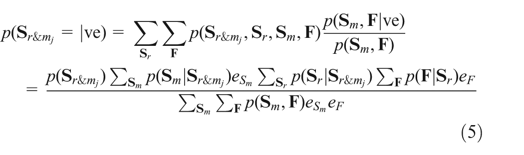
Thus, a probabilities combination is made under the assumption that the model-based method and the data-driven method are conditionally independent to the node added. We can see that the proposed network structure correspond to a NBN with a root node
Once the networks are built, our probabilistic framework is ready to be used for the monitoring task. The inputs or the set of evidence of the proposed method correspond first to the calculated residuals and the observed system variables and second to the outputs of both methods. In this paper, these inputs are propagated following the junction tree principle (Cowell et al., 2007). Once this is done, the node
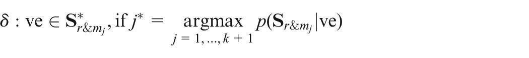
Among other criteria, we choose to use the maximum posterior probability. So, at each instant, the state with the higher posterior probability is taken as
The proposed framework, thanks to its probabilistic aspect, can be an effective way to assist experts in making a decision about the monitored system operating state. For example, this can be done by ranking the different system sates according to their posterior probability of occurrence.
Application
System description
To illustrate the interest of our approach, we use a water heater process (Verron et al., 2009; Weber et al., 2008). It consists of a tank (see Figure 7) equipped with two resistors
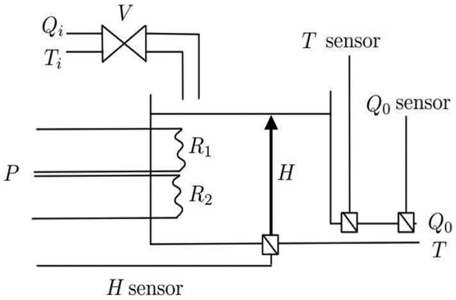
Heating water system.
The thermal system objective is to assure a constant water flow rate at a given temperature. Using the following hydraulic and thermal equations describing the system:
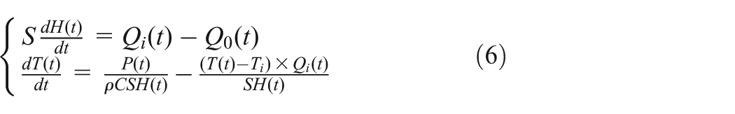
where ρC is a constant thermal variable, S represents the section and Ti is assumed constant and equal to 20°C, a discrete system state space representation around an operating condition (Hop = 0.6 m, Top = 50°C) is determined as follows:
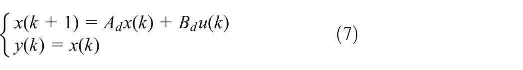
where the output vector y(k) is equal to [T(k) H(k)]T and the input vector u(k) defines [Qi(k) P(k)]T. The sampling period is fixed to 360 seconds in order to respect the closed-loop time constants.
In this analysis, only sensor and components faults are considered:
Using this observer, for each instant k, a residuals vector
Based on the evaluation of
Heating water system incidence matrix.

The framework construction
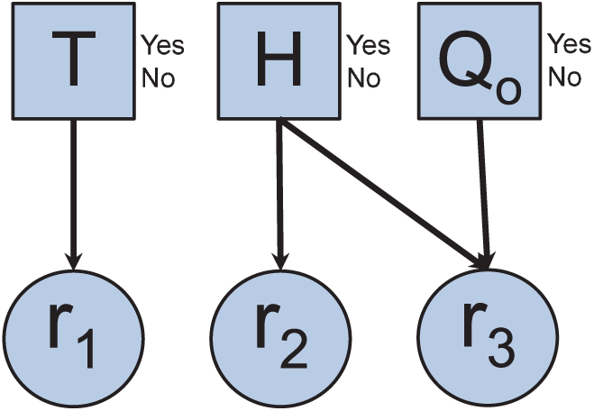
At first, we have to define the two methods for the water heater process. The structures of their corresponding networks are completely different. The one representing the data-driven method corresponds to a linear DA. Its structure is relatively simple (see Figure 8), it links a discrete node representing the different states of the system to a multivariate Gaussian node representing the system variables (m = 3).
Data-driven monitoring.
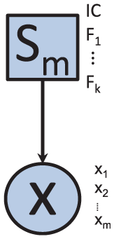
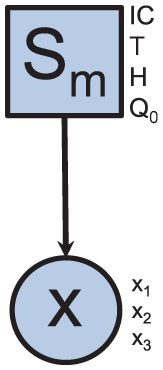
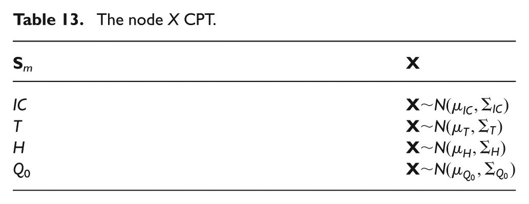
Concerning the one representing the model-based method, it is based on the system incidence matrix (as shown in Figure 9). The different CPTs corresponding to the two graphs are illustrated in Tables 13 and 14.
Model-based monitoring.
The node X CPT.
(a) The nodes
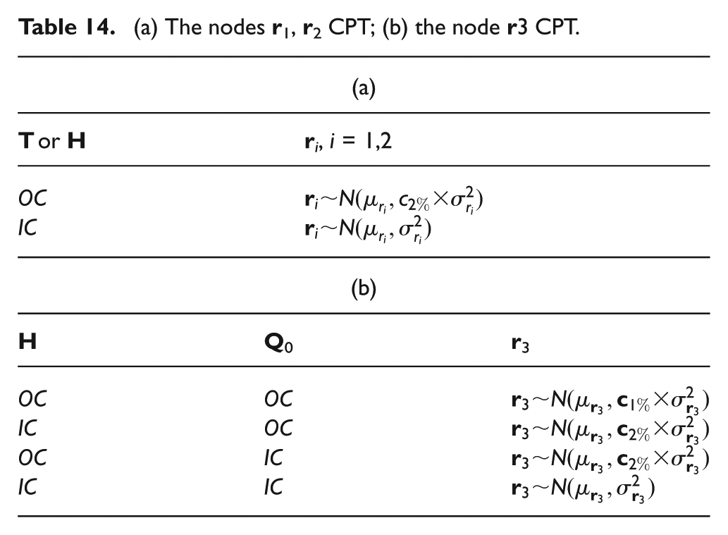
Regarding the CGN presented in Figure 9, the conditional probabilities tables (see Table 14) corresponding to its continuous nodes are defined so that the residual linked to only one fault (see Table 14(b)), is assigned to a 2% as a risk of the first kind (α = 2%). For those connected to more than one fault node, we adopt α = 1%. This choice is made by assuming that a single fault may have a higher false alarm rate than multiple faults. But, since we will not treat multiple faults here, it does not matter if we choose the same α in both cases. The
Once the structure of both networks is established, new discrete nodes
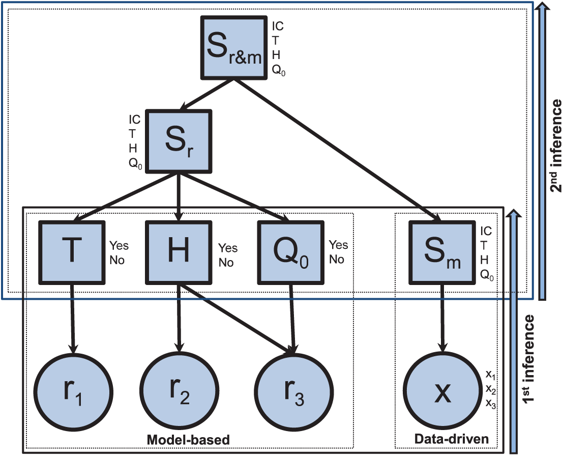
Proposed framework.
The states prior probabilities of the node
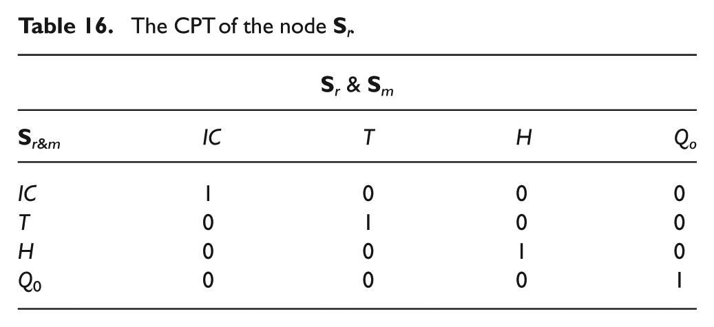
The nodes
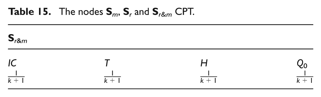
The CPT of the node
Simulations and results
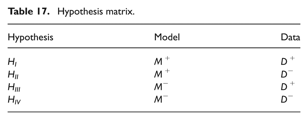
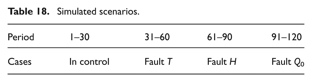
Hereinafter, the proposed method is tested under different assumptions. The value of combining the two methods is mainly to increase the decision reliability. Also, the proposed probabilistic method could be useful when one and/or the other method are not very efficient (abnormal operating state misdetection, faults misdiagnosis). So, we propose to compare our method with the two other networks used alone, taking into account an accurate model (M+) or a less accurate model (M−), and a complete data set of suitable size (D+) or an incomplete data set (lack of fault data, few data available, D−). The scenarios presented previously will be tested on four hypothesis described in Table 17. The system is simulated according to the scenarios described in Table 18.
Hypothesis matrix.
Simulated scenarios.
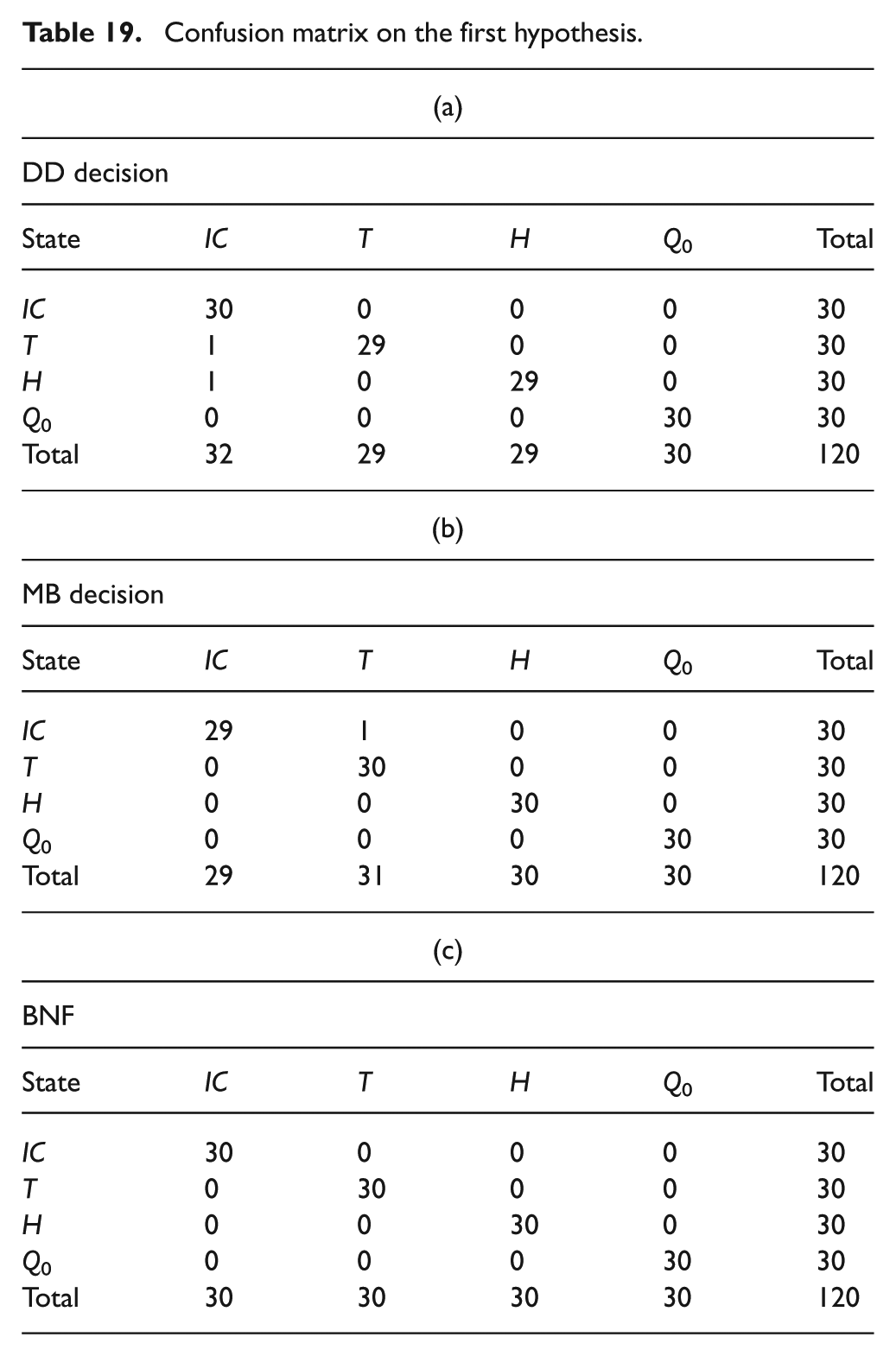
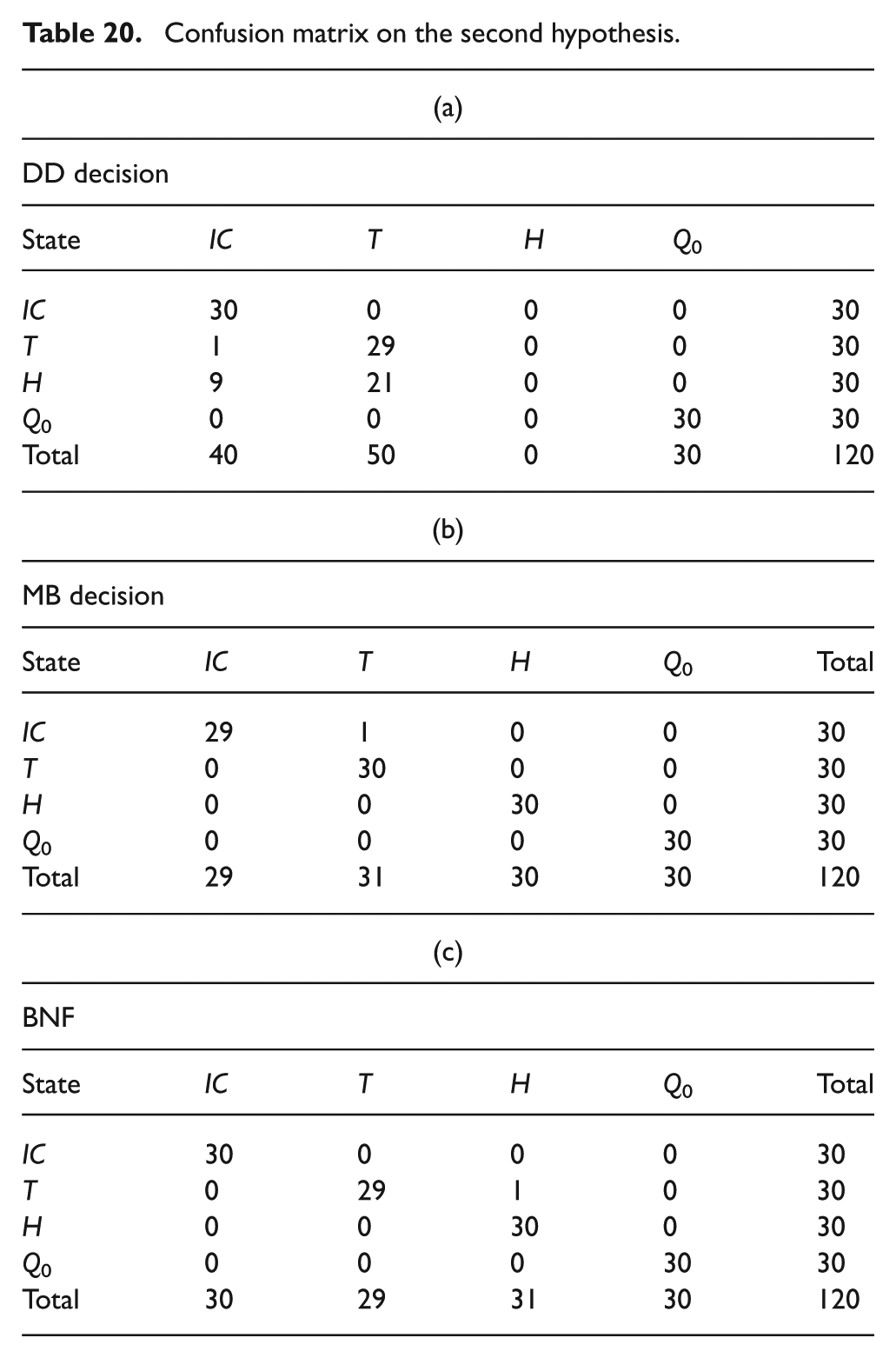
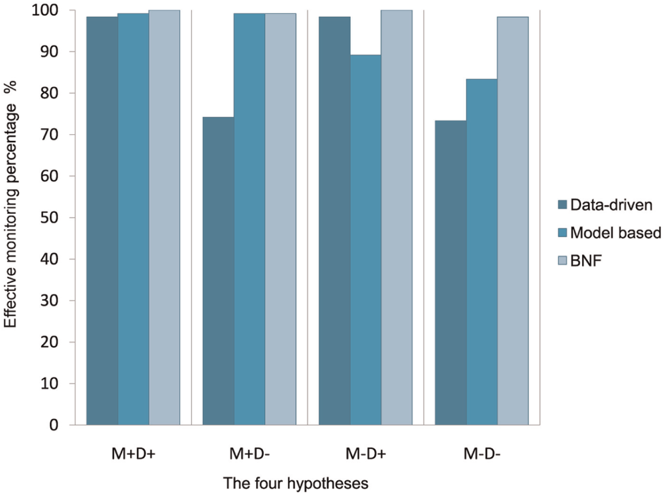
Every simulation was performed using Matlab/Simulink and BNT (Bayes Net Toolbox). The results obtained by testing our methods under four different assumptions are presented in Tables 19, 20, 21 and 22, where each of them represents a confusion matrix. These tables show how the discrimination of the different faults is done, where each column and row of these matrices represent the instances respectively in a predicted class and in an actual class. Moreover, in Figure 11, the comparison of the three methods (DD, data-driven; MB, model-based; BNF, Bayesian networks framework) results under each hypothesis is presented.
Confusion matrix on the first hypothesis.
Confusion matrix on the second hypothesis.
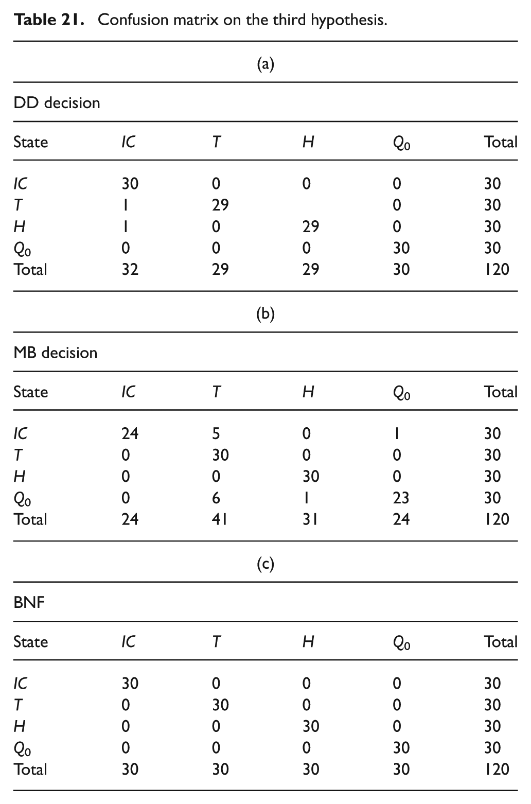
Confusion matrix on the third hypothesis.
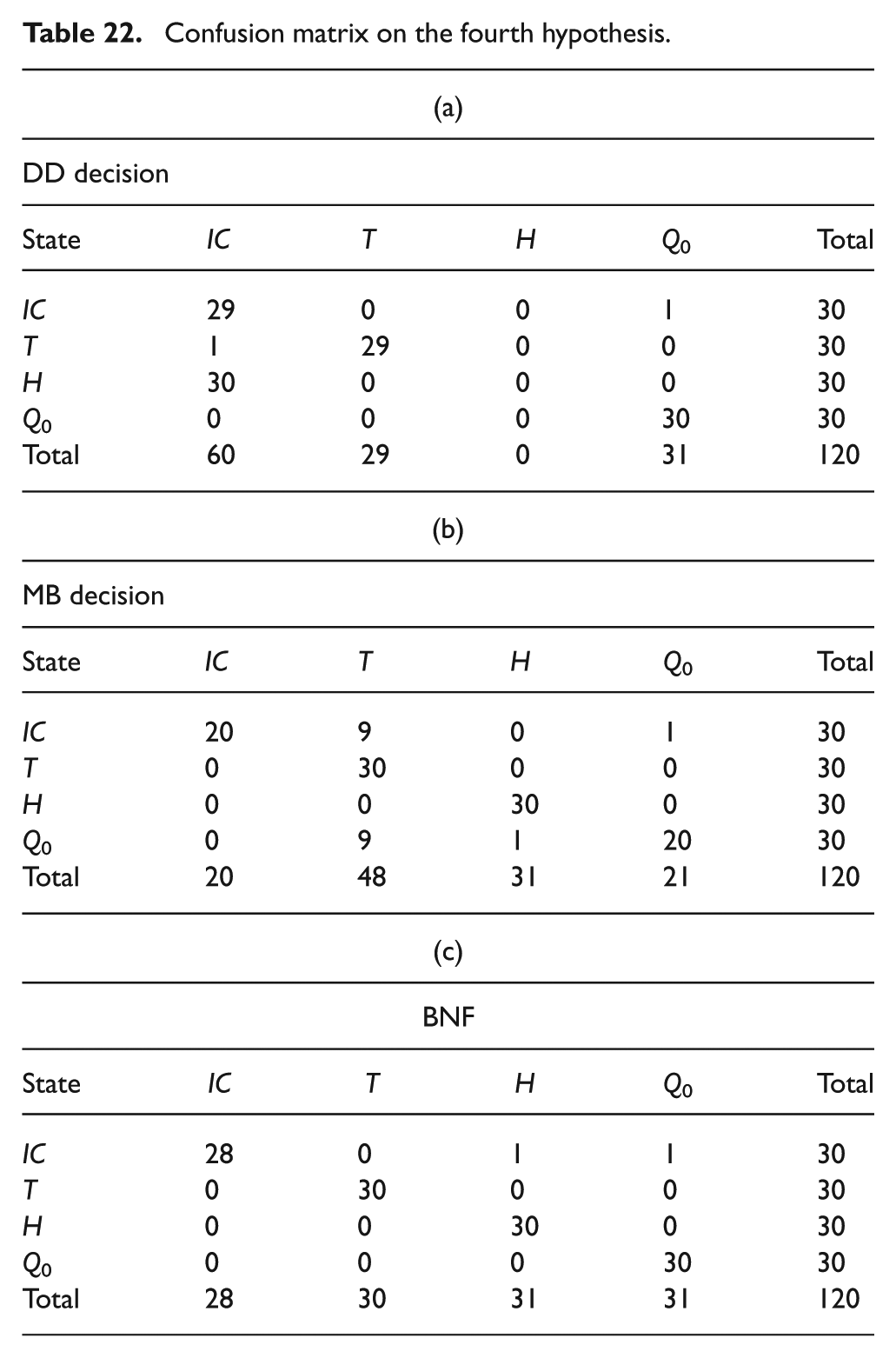
Confusion matrix on the fourth hypothesis.
Results synthesis.
Hypothesis I
In hypothesis (HI), the three methods are used under standard conditions, where an available data set of different faults is used to estimate the needed parameters, and an accurate model (assumed) is provided to generate the residuals. Note that we always consider (for the four hypotheses) that we have enough data when the system is in control. Under these conditions, we see that the three methods are accurate. When the data-driven method made two wrong decisions (error rate: 2/120) and the model-based method made just a one (error rate: 1/120), our method does not make any mistake. These results are deduced from Table 19.
Hypothesis II
Regarding hypothesis II (HII), we consider that there is no data available about the fault H and there is only few data (10 samples) about the other faults (
Hypothesis III
In hypothesis III (HIII), we have made the model less accurate in order to have a model-based method that is less efficient. In the heating water system case, seeking to cause some inaccuracy at the generated residuals, we assume that a physical parameter is incorrectly estimated: the section is set to about 0.35 m2 instead of 1 m2. Under this situation, we see that the proposed method gives good results (does not make any error) comparatively to the model-based method used alone (error rate 13/120). These results can be seen in Table 21.
Hypothesis IV
Finally, in hypothesis IV, we can see that the proposed method allows a better decision (its makes two errors) than the two other methods, where the two conditions made in hypotheses II and III are considered (see Table 22).
Synthesis
One may notice that for each hypothesis, the proposed method can usually approximate or equalize each method performance and even improve the decision making. In hypothesis I, the three methods are good, they give mainly the right answers. In terms of accuracy our method is better. Indeed, it provides more consistency on some states, given the probabilities of the two methods (DD, MB), which could well be useful for experts to make a decision. Concerning the hypothesis II, where we use the data-driven method with a lack of data, the proposed method is relatively good but not as accurate as the model-based method. However, the proposed method has better results than the data-driven method used under an inappropriate environment. The same thing holds, in the case of hypothesis III, where we have degraded the model. Finally, in hypothesis IV the proposed approach made better decisions than the two methods used alone. In this case, it is interesting to see that the two methods under our framework complement each other, as they use different information about the system, to give better decisions. Thus, we can notice that the probabilistic framework can take advantage of the two methods.
Conclusions
The interest of this paper is in presenting a new method for monitoring industrial systems. We have presented a probabilistic framework (i) using discrete and Gaussian variables and (ii) allowing us to model and combine two CGNs for system monitoring: one for data-driven monitoring and the other representing the incidence matrix and the residuals evaluation; two eminent phases in the model-based methods. This framework can enhance decision making during monitoring using data and residuals simultaneously. This original method was tested on a water heater process, where a decision improvement is made and this was in most cases (specific model, degraded model and more or less data) in a natural way. The evident outlook of the proposed approach is, given the proprieties of BNs, to model and integrate other methods or information (maintainability information, components reliability and so on.) about the system in order to further enhance the decision making.
Footnotes
Acknowledgements
The authors gratefully acknowledge the contribution of the reviewers comments.
Funding
Mohamed Amine Atoui is supported by a PhD purpose grant from ‘la Région Pays de la Loire’.