Optimal boundary control of a coupled system consisting of Kuramoto–Sivashinsky–Korteweg

Abstract

This paper is concerned with the optimal boundary control of a non-dimensional non-linear parabolic system consisting of the Kuramoto–Sivashinsky–Korteweg–de Vries equation and a heat equation. By the Dubovitskii and Milyutin functional analytical approach, first in the fixed final horizon case we prove the Pontryagin maximum principle of the optimal control problem of this coupled system. Then under weaker additional conditions, we study the controlled system in the free final horizon case and present further investigational results of current interests. The necessary optimality conditions are established for optimal control problems in these two cases. Finally, a remark on how to utilize the obtained results is also made for illustration.

Keywords

Pontryagin maximum principle optimal boundary control necessary optimality condition parabolic system

Introduction

In the 1970s, when Kuramoto and Tsuzuki (1975) were studying the instabilities on interfaces and flame fronts, a non-linear partial differential equation (PDE) was constructed, which was also reproduced independently by Sivashinsky (1977) during the investigation of phase turbulence in chemical oscillations. This fourth-order PDE was later named the Kuramoto–Sivashinsky (KS) equation and its non-dimensional form reads as

u_{t} (x, t) + δ_{1} u_{xxxx} (x, t) + δ_{2} u_{xx} (x, t) + δ_{3} u (x, t) u_{x} (x, t) = 0

(1)

in which $u (x, t)$ is the real function of the location x and time t, subscripts denote the corresponding partial derivatives, and $δ_{k}, k = 1, 2, 3,$ are parameters. Note that by appropriate rescaling of x, t and u, equation (1) can always be reduced to

u_{t} (x, t) + γ u_{xxxx} (x, t) + a u_{xx} (x, t) + u (x, t) u_{x} (x, t) = 0

In physics, $γ$ and a are coefficients accounting for the long-wave instability and the short-wave dissipation respectively (Malomed et al., 2001).

Since then, this PDE was derived in various physical contexts and also applied in lots of investigations in chemical engineering and mathematical physics including the study into the non-linear stability of falling fluid films, the consideration for the unstable flame front propagation in uniform mixtures, the analysis of the interfacial instabilities in thin-film flows (Annunziato et al., 2000; Matar et al., 2007; Ramaswamy et al., 1996) and so on. It continued to have various kinds of generalisations in different investigational environments. The Kuramoto–Sivashinsky–Korteweg–de Vries (KS–KdV) equation is such a generalization to the KS equation, which introduces a dispersive term $u_{xxx} (x, t)$ from the Korteweg–de Vries (KdV) equation (Malomed et al., 2001). It has the following form

u_{t} (x, t) + γ u_{xxxx} (x, t) + u_{xxx} (x, t) + a u_{xx} (x, t) + u (x, t) u_{x} (x, t) = 0

which is used to model non-linear dissipative waves, but its solitary-pulse (SP) solutions are unstable.

Moreover, to combine dissipative and dispersive features, while simultaneously supporting stable SP, Malomed et al. (2001) introduced a coupled system consisting of the KS–KdV equation (2) and the heat equation (3) below

u_{t} (x, t) + γ u_{xxxx} (x, t) + u_{xxx} (x, t) + a u_{xx} (x, t) + u (x, t) u_{x} (x, t) = v_{x} (x, t)

(2)

v_{t} (x, t) - Γ v_{xx} (x, t) + c v_{x} (x, t) = u_{x} (x, t)

(3)

in which the dissipative parameter $Γ$ accounts for stabilization and c is the group-velocity mismatch between the wave modes (Cerpa et al., 2012). In fact, the linear coupling via the first derivatives is the same as in known models of coupled internal waves propagating in multilayered fluids. The natural physical interpretation of the system above is that it is a model describing a coupled surface and interface waves in a two-layered flowing liquid film. The linear dissipative equation (3) implies that the substrate layer is essentially more viscous than the upper one. In addition, the system of equations (2) and (3) is qualitatively similar to a system of linearly coupled Ginzburg-Landau equations describing the propagation of localized pulses in an fibre-optic core equipped with distributed gain, which is linearly coupled to an extra lossy core that provides for the stability of the pulses; in fact, such double-core systems have recently become available to experimental studies, and they have very promising features for applications to optical communications (Malomed et al., 2001).

By introducing a quadratic term $v^{2} (x, t)$ into the heat equation (3), Cerpa et al. (2012) discussed the boundary controllability of the coupled system consisting of equation (2) and

v_{t} (x, t) - Γ v_{xx} (x, t) + c v_{x} (x, t) + v^{2} (x, t) = u_{x} (x, t)

(4)

and proved its local null-controllability. Beyond that, there are relatively few control problems for these equations in the existing literature. Even for the control of the general KS equation, the investigations are largely unexplored and need more attention. Liu and Krstić (2001) addressed the problem of Dirichlet and Neumann boundary control of the KS equation and developed a Neumann feedback law that guarantees $L^{2} -$ global exponential stability and $H^{2} -$ global asymptotic stability for small values of the anti-diffusion parameter. In Christofides and Armaou (2000), they studied the problem of global exponential stabilization of the one-dimensional KS equation via distributed static output feedback control and showed that the designed scheme stabilizes the KS equation. He et al. (1998) investigated numerical aspects of controllability and optimal control of the KS equation employing the distributed control and periodic boundary conditions. In Yang and Dubljevic (2013), a model modal predictive control (MMPC) strategy was proposed to stabilize the falling liquid film thickness in the vertical tubes modelled by the KS equation in the presence of naturally present state and input constraints. Moreover, they demonstrated that if feasible, the MMPC achieves stabilization of the thin film thickness and satisfies these constraints. By using the adaptive proper orthogonal decomposition (APOD) method, Pourkargar and Armaou (2015) successfully regulated a physico-chemical system that can be described in the form of the KS equation when the process exhibits significant non-linear behaviour. This is a statistical approach which has recently been significantly improved by applying recursive techniques to adaptively revise the required reduced order models as needed during the process operation. The proposed method has been successfully applied to a wide range of non-linear distributed parameter systems over irregular domains to circumvent the traditional POD requirements (a priori availability of a sufficiently large ensemble of PDE solution data) including controller and observer designs. Pourkargar and Armaou (2013) is another important reference on this point. Other interesting references include Armaou and Christofides (2002), Cerpa (2014), Kristić and Smyshlyaev (2008), Lee and Tran (2005), Lenbury et al. (2006) and Sun (2010), to name just a few.

In this paper, we are concerned with the optimal boundary control of the non-dimensional non-linear parabolic system consisting of the KS–KdV equation (2) and the heat equation (4). Let $T > 0$ . The controlled system is constructed as

{\begin{matrix} \begin{matrix} u_{t} (x, t) + γ u_{xxxx} (x, t) + u_{xxx} (x, t) + a u_{xx} (x, t) \\ + u (x, t) u_{x} (x, t) = v_{x} (x, t), \\ v_{t} (x, t) - Γ v_{xx} (x, t) + c v_{x} (x, t) + v^{2} (x, t) = u_{x} (x, t), \\ x \in (0, 1), t \in (0, T), \\ u (0, t) = h_{1} (t) \in L^{2} (0, T), u_{x} (0, t) = h_{2} (t) \in L^{2} (0, T), \\ v (0, t) = h_{3} (t) \in L^{2} (0, T), \\ u (1, t) = 0, u_{x} (1, t) = 0, v (1, t) = 0, \\ u (x, 0) = u_{0} (x) \in H^{- 2} (0, 1), v (x, 0) = v_{0} (x) \in H^{- 1} (0, 1) \end{matrix} \end{matrix}

(5)

where $h_{k}, k = 1, 2, 3,$ are the boundary control inputs, $u_{0}, v_{0}$ are the given initial conditions, $γ$ , a and $Γ$ are assumed to be three positive constants and c is assumed to be constant. In Cerpa et al. (2012), the non-linear system (5) above is proven to satisfy the fact below, which establishes the well-posedness results for the concerned system.

There exists a positive real number r such that for any $u_{0} \in H^{- 2} (0, 1)$ , $v_{0} \in H^{- 1} (0, 1)$ , $h_{1}, h_{2}$ and $h_{3} \in L^{2} (0, T)$ satisfying

∥ (u_{0}, v_{0}) ∥_{H^{- 2} (0, 1) \times H^{- 1} (0, 1)} + ∥ (h_{1}, h_{2}, h_{3}) ∥_{L^{2} {(0, T)}^{3}} \leq r

the non-linear equations (5) have a unique solution $(u, v) \in L^{2} (0, T; L^{2} (0, 1))^{2}$ . Moreover, $(u, v) \in C ([0, T], H^{- 2} (0, 1) \times H^{- 1} (0, 1))$ .

In this article, we will use the results above and suppose, here and now thereafter, unless otherwise stated, that when we speak of a solution of equation (5), we shall always mean the weak solution in this sense.

This paper investigates the optimal control problem of the coupled system (5). By the Dubovitskii and Milyutin functional analytical approach, first in the fixed final horizon case we prove the Pontryagin maximum principle of the optimal control problem of this coupled system. Then under weaker additional conditions, we study the controlled system in the free final horizon case and present further investigational results of current interests. The necessary optimality conditions are established for optimal control problems in these two cases. Finally, a remark on how to utilize the obtained results is also made for illustration.

It is well known that the Pontryagin maximum principle given by L. S. Pontryagin unifies calculus of variations and control theory of ordinary differential equations (Girsanov, 1972; Li and Yong, 1995) and establishes the theoretical basis of modern optimal control theory along with the Bellman dynamic programming principle. In this paper, we commit ourselves to infinite dimensional generalizations of the maximum principle and aim at the optimal control theory of partial differential equations, a subject of much theoretical and practical interest (Li and Yong, 1995). In contrast to the finite dimensional setting, the maximum principle for the infinite dimensional system does not generally hold as a necessary condition for optimal control. Paying particular attention to the time optimal and norm optimal problems, Fattorini (2005) found some optimal controls which either do not satisfy the Pontryagin maximum principle or satisfy it in a certain weak form, which justified this conclusion.

In essence, the necessary optimality condition of the optimal control problem is closely attached to the open-loop control investigations. There is no doubt that the feedback control has many merits compared to the open-loop control. However, the open-loop methods, based on optimal control theory of distributed parameter systems, are known to have advantages of efficiency and accuracy as compared to closed-loop algorithms which are mostly based on the matrix Ricatti equation (Huntley, 1985). In Huntley (1985), a comparative study is made of five methods for calculating the optimal control function for a linear parabolic tracking problem with boundary control. Questions of computational instability, numerical accuracy and economic computer usage are investigated. Open-loop methods based upon the variational equations are shown to have the advantages of efficiency, accuracy and ease of programming. Methods based on the method of lines and the Riccati equation are shown to be less straightforward in use. Moreover, time delays in the implementation of a feedback control system may cause robustness problems and in fact may destabilize the structure in certain cases (Sloss et al., 1998). Moreover, it is impossible to give a general purpose for all kinds of optimal control problems (Ho and Pepyne, 2002). Therefore, it is both necessary and interesting to derive the Pontryagin maximum principle of the coupled system consisting of the KS–KdV equation and the heat equation.

The rest of the paper is organized as follows. In the first subsection of the second section, we will present the first main result of this paper. An optimal boundary control problem in the fixed final horizon case is formulated. By the Dubovitskii–Milyutin theorem, we establish the Pontryagin maximum principle of the optimal boundary control problem in this case. In the following three subsections, the cone of directions of decrease, the cone of feasible directions and the cone of tangent directions as well as their dual cones are, respectively, derived. The proof of the first main result is given in the following subsection. The optimal control system in the free final horizon case is investigated in the third section, and the corresponding Pontryagin maximum principle is likewise obtained. It is our second main result and its proof appears in the final subsection. In the fourth section, a remark on how to utilize the obtained results is made for illustration, and shows the applicability of the obtained results. The fifth section concludes the paper with remarks.

Optimal control in the fixed final horizon case

In this section, we consider the optimal control of the system being investigated in the fixed final horizon case.

The first main result

Let us formulate an optimal control problem for the system (5) with the general cost functional

\min_{h (\cdot) \in U_{a d}} J (u, v, h) = \min_{h (\cdot) \in U_{a d}} \int_{0}^{T} \int_{0}^{1} L (u (x, t), v (x, t), h (t), x, t) d x d t

(6)

and the control constraint

U_{ad} = {h = (h_{1}, h_{2}, h_{3}) \in L^{2} (0, T)^{3} | h_{k} \in U_{k}, k = 1, 2, 3, t \in [0, T] a . e .}

in which every $U_{k}$ , $k = 1, 2, 3,$ is a non-empty closed convex set of $L^{2} (0, T)$ . The integrand L of the double integral in equation (6) is a functional and the assumptions on it will be presented soon afterwards. Note that here, the cost function J is quite general in the sense that it contains most of the practically concerned functions, like the quadratic cost functional of the following form

\begin{array}{l} J (u, v, h) = \int_{0}^{T} \int_{0}^{1} (ℓ_{1} | u (x, t) - u^{†} (x, t) |^{2} + ℓ_{2} | v (x, t) - v^{†} (x, t) |^{2}) d x d t \\ + \sum_{k = 1}^{3} \int_{0}^{T} ℓ_{k + 2} | h_{k} (t) |^{2} d t \end{array}

(7)

where $ℓ_{i} > 0, i = 1, 2, \dots, 5,$ are constant and $(u^{†} (x, t), v^{†} (x, t))$ is the pre-designed optimal state. The control target is to drive the variable $(u, v)$ to match the given desired $(u^{†}, v^{†})$ by adjusting the control function h with minimal energy and work. The second term of the right side of equation (7) reflects the cost of control. In physics, an interesting realization is to formate the stable periodic arrays of the pulses by the control force.

Take $(u, v) \in V_{T} \overset{Δ}{=} C ([0, T], H^{- 2} (0, 1) \times H^{- 1} (0, 1)) \cap L^{2} (0, T; L^{2} (0, 1) \times L^{2} (0, 1))$ . The control space is $L^{2} (0, T)^{3}$ and the control constraint is $h_{k} (t) \in U_{k}, k = 1, 2, 3$ , in $[0, T]$ . Here, we assume that the set $U_{ad}$ of admissible controls has a non-empty interior with respect to $L^{2} (0, T)^{3}$ topology, i.e. ${int}_{L^{2} {(0, T)}^{3}} U_{ad} \neq \emptyset$ , which is an often-used assumption in the literature on the admissible control set (Tröltzsch, 2010). Moreover, one will see that this assumption and even that of the convexity of control set will be removed in the free final horizon case later on. This means that in the free final horizon case, the admissible control set neither needs to be convex nor contain interior points, which is usually regarded as the most difficult situation in extremum problems.

In addition, two assumptions for the cost functional in equation (6) are listed below.

(a) L is a functional defined on $H^{- 2} (0, 1) \times H^{- 1} (0, 1) \times Π_{k = 1}^{3} U_{k} \times [0, 1] \times [0, T]$ and

\frac{\partial L (u (x, t), v (x, t), h (t), x, t)}{\partial u}, \frac{\partial L (u (x, t), v (x, t), h (t), x, t)}{\partial v}, \frac{\partial L (u (x, t), v (x, t), h (t), x, t)}{\partial h_{k}}, k = 1, 2, 3

exist for every $(u, v, h) \in H^{- 2} (0, 1) \times H^{- 1} (0, 1) \times Π_{k = 1}^{3} U_{k}$ and L is continuous in its variables.

(b) The functions

\begin{array}{l} \int_{0}^{1} | \frac{\partial L (u (x, t), v (x, t), h (t), x, t)}{\partial u} | d x, \int_{0}^{1} | \frac{\partial L (u (x, t), v (x, t), h (t), x, t)}{\partial v} | d x, \\ \int_{0}^{1} | \frac{\partial L (u (x, t), v (x, t), h (t), x, t)}{\partial h_{k}} | d x, k = 1, 2, 3 \end{array}

are bounded for $t \in [0, T]$ .

Define $X_{T} = V_{T} \times L^{2} (0, T)^{3}$ . Let $(u^{*}, v^{*}, h^{*})$ be the solution to the optimal control problem (6) subject to equation (5), in which $h^{*} (t) = (h_{1}^{*} (t), h_{2}^{*} (t), h_{3}^{*} (t))$ . Set

\begin{array}{l} Ω_{1} = {(u, v, h) \in X_{T} | h (t) \in U_{a d}, t \in [0, T] a . e .} \\ Ω_{2} = {(u, v, h) \in X_{T} | u_{t} (x, t) + γ u_{x x x x} (x, t) + u_{x x x} (x, t) + a u_{x x} (x, t) + u (x, t) u_{x} (x, t) = v_{x} (x, t) \\ v_{t} (x, t) - Γ v_{x x} (x, t) + c v_{x} (x, t) + v^{2} (x, t) = u_{x} (x, t) \\ u (0, t) = h_{1} (t), u_{x} (0, t) = h_{2} (t), v (0, t) = h_{3} (t) \\ u (1, t) = 0, u_{x} (1, t) = 0, v (1, t) = 0 \\ u (x, 0) = u_{0} (x), v (x, 0) = v_{0} (x) \\ u (x, T) = u^{*} (x, T), v (x, T) = v^{*} (x, T)} \end{array}

Then the problem (6) is equivalent to looking for $(u^{*}, v^{*}, h^{*}) \in Ω = Ω_{1} \cap Ω_{2}$ such that

J (u^{*}, v^{*}, h^{*}) = \min_{(u, v, h) \in Ω} J (u, v, h)

(8)

As a result, we see that the problem (8) has been described into an extremum problem on the constraint $Ω_{1}$ and the equality constraint $Ω_{2}$ . In this situation, the Dubovitskii and Milyutin functional analytical approach has turned out to be very powerful to solve such extremum problems (Chan and Guo, 1989, 1990; Gayte et al., 2010; Girsanov, 1972; Orlov, 1988; Sun, 2010). The general Dubovitskii and Milyutin theorem for the extremum problem (8) can be stated as Theorem 1. We can refer to Girsanov (1972) for the details.

Theorem 1. (Dubovitskii–Milyutin) Suppose the functional $J (u, v, h)$ assumes a minimum at the point $(u^{*}, v^{*}, h^{*})$ in $Ω$ . Assume that $J (u, v, h)$ is regularly decreasing at $(u^{*}, v^{*}, h^{*})$ with the cone of directions of decrease $K_{0}$ , the constraint $Ω_{1}$ is regular at $(u^{*}, v^{*}, h^{*})$ with the cone of feasible directions $K_{1};$ and that the equality constraint $Ω_{2}$ is also regular at $(u^{*}, v^{*}, h^{*})$ with the cone of tangent directions $K_{2}$ . Then there exist continuous linear functionals $f_{0}, f_{1}, f_{2},$ not all identically zero, such that $f_{i} \in K_{i}^{*},$ the dual cone of $K_{i},$ $i = 0, 1, 2,$ which satisfy the condition

f_{0} + f_{1} + f_{2} = 0

(9)

Here, we assume that there exists $(u^{*}, v^{*}, h^{*}) \in Ω$ such that the functional $J (u, v, h)$ assumes a minimum. Under this premise, we present the first order necessary optimality condition of the optimal control problem, which is one of the main results of this paper. Of course, the existence of the optimal solution is also very important in optimal control theory. We will discuss such issues in the future. In addition, although the general Dubovitskii–Milyutin theorem above is given in the settings of problem (6) in the fixed final horizon case, we can construct a similar extremum problem for an optimal control problem in the free final horizon case and give the corresponding theorem. For the sake of brevity, we will not list it for that case, but will directly use this fact during the proof.

In the following, by Theorem 1 above, we will establish the necessary optimality condition of optimal control problem (6) for the coupled system (5) consisting of the KS–KdV equation and a heat equation. The first main result is formulated as Theorem 2.

Theorem 2. Suppose $(u^{*}, v^{*}, h^{*})$ is a solution to the optimal control problem (6). Then there exist $κ_{0} \geq 0$ , $p (x, t)$ and $q (x, t)$ , not identically zero, such that the following maximum principle holds true

\begin{array}{l} (κ_{0} \int_{0}^{1} \frac{\partial L (u^{*}, v^{*}, h^{*}, x, t)}{\partial h_{1}} d x + γ (u_{x x x} (1, t) + p_{x x x} (0, t)) + u_{x x} (1, t) - p_{x x} (0, t)) \cdot (h_{1} (t) - h_{1}^{*} (t)) \\ + (κ_{0} \int_{0}^{1} \frac{\partial L (u^{*}, v^{*}, h^{*}, x, t)}{\partial h_{2}} d x - γ (u_{x x} (1, t) + p_{x x} (0, t))) \cdot (h_{2} (t) - h_{2}^{*} (t)) \\ + (κ_{0} \int_{0}^{1} \frac{\partial L (u^{*}, v^{*}, h^{*}, x, t)}{\partial h_{3}} d x - Γ (v_{x} (1, t) + q_{x x} (0, t))) \cdot (h_{3} (t) - h_{3}^{*} (t)) \geq 0, \\ \forall h (t) \in U_{a d}, t \in [0, T] a . e . \end{array}

(10)

where the function $(p (x, t), q (x, t))$ satisfies the adjoint equation

{\begin{matrix} \begin{matrix} p_{t} (x, t) + (1 - γ) p_{xxx} (x, t) - a p_{xx} (x, t) \\ + u^{*} (x, t) p_{x} (x, t) = q_{x} (x, t) + κ_{0} \frac{\partial L (u^{*}, v^{*}, h^{*}, x, t)}{\partial u} \\ q_{t} (x, t) + Γ q_{xx} (x, t) + c q_{x} (x, t) \\ - 2 v^{*} (x, t) q (x, t) = p_{x} (x, t) + κ_{0} \frac{\partial L (u^{*}, v^{*}, h^{*}, x, t)}{\partial v} \\ p (0, t) = 0, p_{x} (0, t) = 0, q (0, t) = 0 \\ p (1, t) = h_{1} (t), p_{x} (1, t) = h_{2} (t), q (1, t) = h_{3} (t) \\ p (x, T) = ϕ (x), q (x, T) = ψ (x) \end{matrix} \end{matrix}

(11)

in which $ϕ (x) \in H_{0}^{2} (0, 1)$ and $ψ (x) \in H_{0}^{1} (0, 1)$ are given in equation (18).

The proof of this theorem appears in the final subsection.

The cone of directions of decrease K₀

To prove Theorem 2, we need to determine the cone of directions of decrease $K_{0}$ , the cone of feasible directions $K_{1}$ , the cone of tangent directions $K_{2}$ and their corresponding dual cones $K_{i}^{*},$ $i = 0, 1, 2$ . Moreover, in these dual cones, we must derive the continuous linear functionals $f_{i},$ $i = 0, 1, 2 .$ Then, step by step, by condition (9), establish the Pontryagin maximum principle of optimal control problem (6).

First we must find the cone of directions of decrease $K_{0}$ . By the assumptions for the cost functional given above, $J (u, v, h)$ is differentiable at any point $(u^{0}, v^{0}, h^{0})$ in any direction $(u, v, h)$ and its directional derivative is

\begin{array}{l} J^{'} (u^{0}, v^{0}, h^{0}; u, v, h) \\ = \lim_{ε \to 0 +} \frac{1}{ε} (J (u^{0} + ε u, v^{0} + ε v, h^{0} + ε h) - J (u^{0}, v^{0}, h^{0})) \\ = \lim_{ε \to 0 +} \frac{1}{ε} {\int_{0}^{T} \int_{0}^{1} (L (u^{0} + ε u, v^{0} + ε v, h^{0} + ε h, x, t) - L (u^{0}, v^{0}, h^{0}, x, t)) d x d t} \\ = \int_{0}^{T} \int_{0}^{1} (\frac{\partial L (u^{0}, v^{0}, h^{0}, x, t)}{\partial u} u + \frac{\partial L (u^{0}, v^{0}, h^{0}, x, t)}{\partial v} v + \sum_{k = 1}^{3} \frac{\partial L (u^{0}, v^{0}, h^{0}, x, t)}{\partial h_{k}} h_{k}) d x d t \end{array}

The cone of directions of decrease of the functional $J (u, v, h)$ at point $(u^{*}, v^{*}, h^{*})$ is thereupon determined by

\begin{array}{l} K_{0} = {(u, v, h) \in X_{T} | J^{'} (u^{*}, v^{*}, h^{*}; u, v, h) < 0} \\ = {(u, v, h) \in X_{T} | \int_{0}^{T} \int_{0}^{1} (\frac{\partial L (u^{*}, v^{*}, h^{*}, x, t)}{\partial u} u \\ + \frac{\partial L (u^{*}, v^{*}, h^{*}, x, t)}{\partial v} v + \sum_{k = 1}^{3} \frac{\partial L (u^{*}, v^{*}, h^{*}, x, t)}{\partial h_{k}} h_{k}) d x d t < 0} \end{array}

If $K_{0} \neq \emptyset$ , then for any $f_{0} \in K_{0}^{*}$ , the dual cone of $K_{0}$ , there exists a $κ_{0} \geq 0$ such that

\begin{matrix} f_{0} (u, v, h) = - κ_{0} \int_{0}^{T} \int_{0}^{1} (\frac{\partial L (u^{*}, v^{*}, h^{*}, x, t)}{\partial u} u \\ + \frac{\partial L (u^{*}, v^{*}, h^{*}, x, t)}{\partial v} v + \sum_{k = 1}^{3} \frac{\partial L (u^{*}, v^{*}, h^{*}, x, t)}{\partial h_{k}} h_{k}) dx dt \end{matrix}

The cone of feasible directions $K_{1}$

Secondly, for the cone of feasible directions $K_{1}$ , since $Ω_{1} = V_{T} \times U_{ad}$ , in which ${int}_{L^{2} {(0, T)}^{3}} U_{ad} \neq \emptyset$ , the interior of $Ω_{1}$ is not empty, i.e. ${Ω^{o}}_{1} \neq \emptyset$ At point $(u^{*}, v^{*}, h^{*})$ , the cone of feasible directions $K_{1}$ of $Ω_{1}$ is determined by

\begin{array}{l} K_{1} = {κ ({\overset{o}{Ω}}_{1} - (u^{*}, v^{*}, h^{*})) | κ > 0} \\ = {ρ | ρ = κ (u - u^{*}, v - v^{*}, h - h^{*}), (u, v, h) \in {\overset{o}{Ω}}_{1}, κ > 0} \end{array}

As a result, for an arbitrary $f_{1} \in K_{1}^{*}$ , the dual cone of $K_{1}$ , if there is an $\bar{a} (t) = ({\bar{a}}_{1} (t), {\bar{a}}_{2} (t), {\bar{a}}_{3} (t)) \in L^{2} (0, T)^{3},$ such that the linear functional defined by

f_{1} (u, v, h) = \sum_{k = 1}^{3} \int_{0}^{T} {\bar{a}}_{k} (t) h_{k} (t) dt

(12)

is a support to $U_{ad}$ at point $h^{*}$ , then

\sum_{k = 1}^{3} {\bar{a}}_{k} (t) (h_{k} (t) - h_{k}^{*} (t)) \geq 0, \forall h (t) \in U_{ad}, t \in [0, T] a . e .

(13)

The cone of tangent directions $K_{2}$

Next we derive the cone of tangent directions $K_{2}$ . Let ${\bar{V}}_{T} = L^{2} (0, T; H^{- 6} (0, 1)) \cap H^{- 1} (0, T; H^{- 4} (0, 1)$ and ${\tilde{V}}_{T} = L^{2} (0, T; H^{- 3} (0, 1)) \cap H^{- 1} (0, T; H^{- 2} (0, 1)$ . Define the operator $G : X_{T} \to {\bar{V}}_{T} \times {\tilde{V}}_{T} \times L^{2} (0, T)^{6} \times (H^{- 2} (0, 1) \times H^{- 1} (0, 1))^{2}$ by

\begin{array}{l} G (u, v, h) = (u_{t} (x, t) + γ u_{x x x x} (x, t) + u_{x x x} (x, t) \\ + a u_{x x} (x, t) + u (x, t) u_{x} (x, t) - v_{x} (x, t), \\ v_{t} (x, t) - Γ v_{x x} (x, t) + c v_{x} (x, t) + v^{2} (x, t) - u_{x} (x, t), \\ u (0, t) - h_{1} (t), u_{x} (0, t) - h_{2} (t), v (0, t) - h_{3} (t), \\ u (1, t), u_{x} (1, t), v (1, t), u (x, 0) - u_{0} (x), \\ v (x, 0) - v_{0} (x), u (x, T) - u^{*} (x, T), v (x, T) - v^{*} (x, T)) \end{array}

Then

Ω_{2} = {(u, v, h) \in X_{T} | G (u (x, t), v (x, t), h (t)) = 0}

The Fréchet-derivative of the operator $G (u, v, h)$ is

\begin{array}{l} G^{'} (u, v, h) (\hat{u}, \hat{v}, \hat{h}) \\ = ({\hat{u}}_{t} (x, t) + γ {\hat{u}}_{x x x x} (x, t) + {\hat{u}}_{x x x} (x, t) + a {\hat{u}}_{x x} (x, t) \\ + u (x, t) {\hat{u}}_{x} (x, t) + \hat{u} (x, t) u_{x} (x, t) - {\hat{v}}_{x} (x, t), \\ {\hat{v}}_{t} (x, t) - Γ {\hat{v}}_{x x} (x, t) + c {\hat{v}}_{x} (x, t) + 2 v (x, t) \hat{v} (x, t) \\ - {\hat{u}}_{x} (x, t), \hat{u} (0, t) - {\hat{h}}_{1} (t), {\hat{u}}_{x} (0, t) - {\hat{h}}_{2} (t), \hat{v} (0, t) \\ - {\hat{h}}_{3} (t), \hat{u} (1, t), {\hat{u}}_{x} (1, t), \hat{v} (1, t), \\ \hat{u} (x, 0), \hat{v} (x, 0), \hat{u} (x, T), \hat{v} (x, T)) \end{array}

Since $(u^{*}, v^{*}, h^{*})$ is the solution to the problem (6), it has $G (u^{*}, v^{*}, h^{*}) = 0$ . Choosing arbitrary

(g_{1}, g_{2}, g_{3}, g_{4}, g_{5}, g_{6}, g_{7}, g_{8}, g_{9}, g_{10}, g_{11}, g_{12}) \in {\bar{V}}_{T} \times {\tilde{V}}_{T} \times L^{2} (0, T)^{6} \times (H^{- 2} (0, 1) \times H^{- 1} (0, 1))^{2}

and solving the equation

\begin{array}{l} G^{'} (u^{*}, v^{*}, h^{*}) (\hat{u}, \hat{v}, \hat{h}) = (g_{1} (x, t), g_{2} (x, t), g_{3} (t), g_{4} (t), g_{5} (t), \\ g_{6} (t), g_{7} (t), g_{8} (t), g_{9} (x), g_{10} (x), g_{11} (x), g_{12} (x)) \end{array}

we obtain

{\begin{cases} {\hat{u}}_{t} (x, t) + γ {\hat{u}}_{x x x x} (x, t) + {\hat{u}}_{x x x} (x, t) + a {\hat{u}}_{x x} (x, t) \\ + u^{*} (x, t) {\hat{u}}_{x} (x, t) + \hat{u} (x, t) u_{x}^{*} (x, t) - {\hat{v}}_{x} (x, t) = g_{1} (x, t) \\ {\hat{v}}_{t} (x, t) - Γ {\hat{v}}_{x x} (x, t) + c {\hat{v}}_{x} (x, t) + 2 v^{*} (x, t) \hat{v} (x, t) - {\hat{u}}_{x} (x, t) = g_{2} (x, t) \\ \hat{u} (0, t) - {\hat{h}}_{1} (t) = g_{3} (t), {\hat{u}}_{x} (0, t) - {\hat{h}}_{2} (t) = g_{4} (t), \hat{v} (0, t) - {\hat{h}}_{3} (t) = g_{5} (t) \\ \hat{u} (1, t) = g_{6} (t), {\hat{u}}_{x} (1, t) = g_{7} (t), \hat{v} (1, t) = g_{8} (t) \\ \hat{u} (x, 0) = g_{9} (x), \hat{v} (x, 0) = g_{10} (x), \hat{u} (x, T) = g_{11} (x), \hat{v} (x, T) = g_{12} (x) \end{cases}

(14)

Here, assume that the linearized system

{\begin{matrix} u_{t} (x, t) + γ u_{xxxx} (x, t) + u_{xxx} (x, t) + a u_{xx} (x, t) \\ + u^{*} (x, t) u_{x} (x, t) + u (x, t) u_{x}^{*} (x, t) = v_{x} (x, t) \\ v_{t} (x, t) - Γ v_{xx} (x, t) + c v_{x} (x, t) + 2 v^{*} (x, t) v (x, t) = u_{x} (x, t) \\ u (0, t) = h_{1} (t), u_{x} (0, t) = h_{2} (t), v (0, t) = h_{3} (t) \\ u (1, t) = 0, u_{x} (1, t) = 0, v (1, t) = 0 \\ u (x, 0) = 0, v (x, 0) = 0 \end{matrix}

(15)

is controllable (refer to Chan and Guo (1989, 1990) for information on the linearization). Then choose $h (t) = \hat{h} (t) \in L^{2} (0, T)^{3}$ such that $u (x, T) = g_{11} (x) - ξ (x, T)$ , $v (x, T) = g_{12} (x) - η (x, T)$ , and let $(u, v)$ be the solution to the linearized system (15). Choose $\hat{u} (x, t) = u (x, t) + ξ (x, t)$ , $\hat{v} (x, t) = v (x, t) + η (x, t)$ , where $(ξ, η)$ satisfies the following equations

{\begin{matrix} \begin{matrix} ξ_{t} (x, t) + γ ξ_{xxxx} (x, t) + ξ_{xxx} (x, t) + a ξ_{xx} (x, t) \\ + u^{*} (x, t) ξ_{x} (x, t) + ξ (x, t) u_{x}^{*} (x, t) - η_{x} (x, t) = g_{1} (x, t) \\ η_{t} (x, t) - Γ η_{xx} (x, t) + c η_{x} (x, t) + 2 v^{*} (x, t) η (x, t) \\ - ξ_{x} (x, t) = g_{2} (x, t) \\ ξ (0, t) = g_{3} (t), ξ_{x} (0, t) = g_{4} (t), η (0, t) = g_{5} (t) \\ ξ (1, t) = g_{6} (t), ξ_{x} (1, t) = g_{7} (t), η (1, t) = g_{8} (t) \\ ξ (x, 0) = g_{9} (x), η (x, 0) = g_{10} (x) \end{matrix} \end{matrix}

In this way, it suffices for $(\hat{u}, \hat{v}, \hat{h})$ to satisfy equation (14). Therefore $G' (u^{*}, v^{*}, h^{*})$ maps the space $X_{T}$ onto ${\bar{V}}_{T} \times {\tilde{V}}_{T} \times L^{2} (0, T)^{6} \times (H^{- 2} (0, 1) \times H^{- 1} (0, 1))^{2}$ . Moreover, the cone of the tangent directions $K_{2}$ to the constraint $Ω_{2}$ at point $(u^{*}, v^{*}, h^{*})$ consists of the kernel of $G' (u^{*}, v^{*}, h^{*})$ , i.e. $(u, v, h)$ satisfies the following equations in $X_{T}$

{\begin{matrix} \begin{matrix} u_{t} (x, t) + γ u_{xxxx} (x, t) + u_{xxx} (x, t) + a u_{xx} (x, t) \\ + u^{*} (x, t) u_{x} (x, t) + u (x, t) u_{x}^{*} (x, t) = v_{x} (x, t) \\ v_{t} (x, t) - Γ v_{xx} (x, t) + c v_{x} (x, t) + 2 v^{*} (x, t) v (x, t) = u_{x} (x, t) \\ u (0, t) = h_{1} (t), u_{x} (0, t) = h_{2} (t), v (0, t) = h_{3} (t) \\ u (1, t) = 0, u_{x} (1, t) = 0, v (1, t) = 0 \\ u (x, 0) = 0, v (x, 0) = 0 \end{matrix} \end{matrix}

(16)

and

u (x, T) = 0, v (x, T) = 0

(17)

Let

\begin{matrix} K_{21} = {(u, v, h) \in X_{T} | (u (x, t), v (x, t), h (t)) satisfies (16)} \\ K_{22} = {(u, v, h) \in X_{T} | (u (x, t), v (x, t), h (t)) satisfies (17)} \end{matrix}

Then the cone of tangent directions $K_{2} = K_{21} ⋂ K_{22}$ . Consequently

K_{2}^{*} = K_{21}^{*} + K_{22}^{*}

For any $f_{2} \in K_{2}^{*}$ , decompose $f_{2} = f_{21} + f_{22}, f_{2 i} \in K_{2 i}^{*}$ , the dual cone of $K_{2 i}, i = 1, 2$ . Moreover, $f_{21} (u, v, h) = 0$ and for all $(u (x, t), v (x, t)) \in V_{T}$ satisfying $u (x, T) = 0, v (x, T) = 0$ , there exist $ϕ (x) \in H_{0}^{2} (0, 1), ψ (x) \in H_{0}^{1} (0, 1)$ such that

f_{22} (u, v, h) = \int_{0}^{1} (u (x, T) ϕ (x) + v (x, T) ψ (x)) dx

(18)

It then follows from Theorem 1 that there exist continuous linear functionals, not all identically zero, such that

f_{0} + f_{1} + f_{21} + f_{22} = 0

Therefore, when selecting $(u, v, h)$ that satisfies (16), $f_{21} (u, v, h) = 0$ . We have

\begin{array}{l} f_{1} (u, v, h) = - f_{0} (u, v, h) - f_{22} (u, v, h) \\ = κ_{0} \int_{0}^{T} \int_{0}^{1} \frac{\partial L (u^{*}, v^{*}, h^{*}, x, t)}{\partial u} u + \frac{\partial L (u^{*}, v^{*}, h^{*}, x, t)}{\partial v} v \\ + \sum_{k = 1}^{3} \frac{\partial L (u^{*}, v^{*}, h^{*}, x, t)}{\partial h_{k}} h_{k} d x d t \\ - \int_{0}^{1} (u (x, T) ϕ (x) + v (x, T) ψ (x)) d x \end{array}

Maximum principle of problem (6)

Now we are only one step away from obtaining the necessary optimality condition and establishing the Pontryagin maximum principle for problem (6). For this purpose, we need to formulate the adjoint system of equation (15). Here, define the adjoint system as equation (11). As with equation (5), the existence and uniqueness of solution to the adjoint system can be obtained in a similar way.

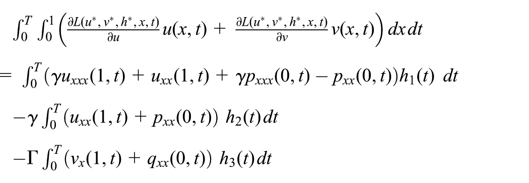
Theorem 3. The solution of system (15) and that of its adjoint system (11) have the following relationship

\begin{matrix} \begin{matrix} \int_{0}^{1} (u (x, T) ϕ (x) + v (x, T) ψ (x)) dx \\ - κ_{0} \int_{0}^{T} \int_{0}^{1} (\frac{\partial L (u^{*}, v^{*}, h^{*}, x, t)}{\partial u} u (x, t) + \frac{\partial L (u^{*}, v^{*}, h^{*}, x, t)}{\partial v} v (x, t)) dx dt \\ = \int_{0}^{T} (- γ u_{xxx} (1, t) - u_{xx} (1, t) - γ p_{xxx} (0, t) + p_{xx} (0, t)) h_{1} (t) dt \\ + γ \int_{0}^{T} (u_{xx} (1, t) + p_{xx} (0, t)) h_{2} (t) dt \\ + Γ \int_{0}^{T} (v_{x} (1, t) + q_{xx} (0, t)) h_{3} (t) dt \end{matrix} \end{matrix}

Proof. Multiply the first equation in (11) by $u (x, t)$ and integrate the product by parts over $[0, 1] \times [0, T]$ with respect to x and t respectively. Similarly, multiply the second equation by $v (x, t)$ in equation (11) and have the integration by parts over $[0, 1] \times [0, T]$ . The proof then follows the sum of two integrals above. □

In what follows, we will prove the first main result.

Proof of Theorem 2

By virtue of Theorem 3, we can rewrite $f_{1} (u, v, h)$ as

\begin{matrix} \begin{matrix} f_{1} (u, v, h) = \int_{0}^{T} {κ_{0} \sum_{k = 1}^{3} h_{k} (t) \int_{0}^{1} \frac{\partial L (u^{*}, v^{*}, h^{*}, x, t)}{\partial h_{k}} dx \\ + (γ u_{xxx} (1, t) + u_{xx} (1, t) + γ p_{xxx} (0, t) - p_{xx} (0, t)) h_{1} (t) \\ - γ (u_{xx} (1, t) + p_{xx} (0, t)) h_{2} (t) - Γ (v_{x} (1, t) + q_{xx} (0, t)) h_{3} (t)} dt \end{matrix} \end{matrix}

In view of equation (12)

\bar{a} (t) = {(\begin{matrix} \begin{matrix} κ_{0} \int_{0}^{1} \frac{\partial L (u^{*}, v^{*}, h^{*}, x, t)}{\partial h_{1}} dx + γ (u_{xxx} (1, t) + p_{xxx} (0, t)) \\ + u_{xx} (1, t) - p_{xx} (0, t) \\ κ_{0} \int_{0}^{1} \frac{\partial L (u^{*}, v^{*}, h^{*}, x, t)}{\partial h_{2}} dx - γ (u_{xx} (1, t) + p_{xx} (0, t)) \\ κ_{0} \int_{0}^{1} \frac{\partial L (u^{*}, v^{*}, h^{*}, x, t)}{\partial h_{3}} dx - Γ (v_{x} (1, t) + q_{xx} (0, t)) \end{matrix} \end{matrix})}^{T}

and equation (13) then reads as

\begin{array}{l} (κ_{0} \int_{0}^{1} \frac{\partial L (u^{*}, v^{*}, h^{*}, x, t)}{\partial h_{1}} d x + γ (u_{x x x} (1, t) + p_{x x x} (0, t)) + u_{x x} (1, t) - p_{x x} (0, t)) \\ \cdot (h_{1} (t) - h_{1}^{*} (t)) \\ + (κ_{0} \int_{0}^{1} \frac{\partial L (u^{*}, v^{*}, h^{*}, x, t)}{\partial h_{2}} d x - γ (u_{x x} (1, t) + p_{x x} (0, t))) \cdot (h_{2} (t) - h_{2}^{*} (t)) \\ + (κ_{0} \int_{0}^{1} \frac{\partial L (u^{*}, v^{*}, h^{*}, x, t)}{\partial h_{3}} d x - Γ (v_{x} (1, t) + q_{x x} (0, t))) \cdot (h_{3} (t) - h_{3}^{*} (t)) \geq 0, \\ \forall h (t) \in U_{a d}, t \in [0, T] a . e . \end{array}

(19)

where the superscript ^T denotes the transpose of a vector as well as $κ_{0}$ , $p (x, t)$ and $q (x, t)$ are not identical to zero simultaneously, since otherwise there are definitely $f_{0} = 0, f_{1} = 0, f_{22} = 0$ and $f_{21} = 0$ , which contradict the fact in Theorem 1 that these continuous linear functionals are not all identically zero.

On the other hand, if $K_{0}$ is a null set, then there is

\begin{matrix} \begin{matrix} \int_{0}^{T} \int_{0}^{1} (\frac{\partial L (u^{*}, v^{*}, h^{*}, x, t)}{\partial u} u (x, t) + \frac{\partial L (u^{*}, v^{*}, h^{*}, x, t)}{\partial v} v (x, t) \\ + \sum_{k = 1}^{3} \frac{\partial L (u^{*}, v^{*}, h^{*}, x, t)}{\partial h_{k}} h_{k} (t)) dx dt = 0, \forall (u, v, h) \in X_{T} \end{matrix} \end{matrix}

In particular, if we choose $κ_{0} = 1$ , $ϕ (x) = 0$ and $ψ (x) = 0$ , it then follows from Theorem 3 that

\begin{matrix} \begin{matrix} \int_{0}^{T} \int_{0}^{1} (\frac{\partial L (u^{*}, v^{*}, h^{*}, x, t)}{\partial u} u (x, t) + \frac{\partial L (u^{*}, v^{*}, h^{*}, x, t)}{\partial v} v (x, t)) dx dt \\ = \int_{0}^{T} (γ u_{xxx} (1, t) + u_{xx} (1, t) + γ p_{xxx} (0, t) - p_{xx} (0, t)) h_{1} (t) dt \\ - γ \int_{0}^{T} (u_{xx} (1, t) + p_{xx} (0, t)) h_{2} (t) dt \\ - Γ \int_{0}^{T} (v_{x} (1, t) + q_{xx} (0, t)) h_{3} (t) dt \end{matrix} \end{matrix}

Thus

\begin{matrix} \begin{matrix} \int_{0}^{T} \int_{0}^{1} \sum_{k = 1}^{3} \frac{\partial L (u^{*}, v^{*}, h^{*}, x, t)}{\partial h_{k}} h_{k} (t) dx dt \\ + \int_{0}^{T} (γ u_{xxx} (1, t) + u_{xx} (1, t) + γ p_{xxx} (0, t) - p_{xx} (0, t)) h_{1} (t) dt \\ - γ \int_{0}^{T} (u_{xx} (1, t) + p_{xx} (0, t)) h_{2} (t) dt \\ - Γ \int_{0}^{T} (v_{x} (1, t) + q_{xx} (0, t)) h_{3} (t) dt = 0, \\ \forall h (t) \in L^{2} (0, T)^{3} \end{matrix} \end{matrix}

from which we obtain

\begin{matrix} \begin{matrix} \sum_{k = 1}^{3} h_{k} (t) \int_{0}^{1} \frac{\partial L (u^{*}, v^{*}, h^{*}, x, t)}{\partial h_{k}} dx \\ + (γ u_{xxx} (1, t) + u_{xx} (1, t) + γ p_{xxx} (0, t) - p_{xx} (0, t)) h_{1} (t) \\ - γ (u_{xx} (1, t) + p_{xx} (0, t)) h_{2} (t) \\ - Γ (v_{x} (1, t) + q_{xx} (0, t)) h_{3} (t) = 0, \forall t \in [0, T] a . e . \end{matrix} \end{matrix}

Therefore equation (19) still holds.

In addition, if there is a non-zero solution $(\hat{p} (x, t), \hat{q} (x, t))$ to the adjoint system

{\begin{matrix} \begin{matrix} {\hat{p}}_{t} (x, t) + (1 - γ) {\hat{p}}_{xxx} (x, t) - a {\hat{p}}_{xx} (x, t) \\ + u^{*} (x, t) {\hat{p}}_{x} (x, t) = {\hat{q}}_{x} (x, t) + κ_{0} \frac{\partial L (u^{*}, v^{*}, h^{*}, x, t)}{\partial u} \\ {\hat{q}}_{t} (x, t) + Γ {\hat{q}}_{xx} (x, t) + c {\hat{q}}_{x} (x, t) \\ - 2 v^{*} (x, t) \hat{q} (x, t) = {\hat{p}}_{x} (x, t) + κ_{0} \frac{\partial L (u^{*}, v^{*}, h^{*}, x, t)}{\partial v} \\ \hat{p} (0, t) = 0, {\hat{p}}_{x} (0, t) = 0, \hat{q} (0, t) = 0 \\ \hat{p} (1, t) = h_{1} (t), {\hat{p}}_{x} (1, t) = h_{2} (t), \hat{q} (1, t) = h_{3} (t) \\ \hat{p} (x, T) = ϕ (x), \hat{q} (x, T) = ψ (x) \end{matrix} \end{matrix}

(20)

such that the following equality holds true

b (t) = (\begin{matrix} γ (u_{xxx} (1, t) + {\hat{p}}_{xxx} (0, t)) + u_{xx} (1, t) - {\hat{p}}_{xx} (0, t) \\ γ (u_{xx} (1, t) + {\hat{p}}_{xx} (0, t)) \\ Γ (v_{x} (1, t) + {\hat{q}}_{xx} (0, t)) \end{matrix}) = 0, \forall t \in [0, T] a . e .

then when we choose $κ_{0} = 0$ , $ϕ (x) = \hat{p} (x, T)$ and $ψ (x) = \hat{q} (x, T)$ , equation (19) is still valid. Otherwise, for any non-zero solution $(\hat{p}, \hat{q})$ of equation (20), $b (t) ≢ 0$ , and in this case we say the situation is non-degenerate. Then the linearized system (15) is controllable. In fact, if system (15) is not controllable, then there exist $ϕ (x) \in H_{0}^{2} (0, 1), ψ (x) \in H_{0}^{1} (0, 1)$ such that

\int_{0}^{1} (u (x, T) ϕ (x) + v (x, T) ψ (x)) dx = 0, ϕ (x) ≢ 0, ψ (x) ≢ 0

Choose $κ_{0} = 0$ , $(\hat{p}, \hat{q})$ to be the solution of equation (20). Then it follows from Theorem 3 that

\begin{matrix} \begin{matrix} \int_{0}^{T} (- γ u_{xxx} (1, t) - u_{xx} (1, t) - γ p_{xxx} (0, t) + p_{xx} (0, t)) h_{1} (t) dt \\ + γ \int_{0}^{T} (u_{xx} (1, t) + p_{xx} (0, t)) h_{2} (t) dt \\ + Γ \int_{0}^{T} (v_{x} (1, t) + q_{xx} (0, t)) h_{3} (t) dt = 0, \\ \forall h (t) \in L^{2} (0, T)^{3} \end{matrix} \end{matrix}

Thus

b (t) = 0, \forall t \in [0, T] a . e .

which is a contradiction. In the case of equation (20), the system (15) is consequently controllable.

Combining the results above, we have obtained the Pontryagin maximum principle (10) for the problem (6) subject to the system (5). This completes the proof of our first main result. □

Optimal control in free final horizon case

In the second section, we gave the Pontryagin maximum principle for the optimal control problem (6) of system (5) in the fixed final horizon case. The result is derived under two additional conditions. The first is that the admissible control set must be convex, and the second requires the cost functional to be differentiable with respect to the control variable. In this section, we consider the system with free final time without these assumptions.

The second main result

Consider the following control system defined in the fixed domain $[0, 1] \times [0, t_{1}]$

{\begin{cases} u_{t} (x, t) + γ u_{x x x x} (x, t) + u_{x x x} (x, t) + a u_{x x} (x, t) \\ + u (x, t) u_{x} (x, t) = v_{x} (x, t) \\ v_{t} (x, t) - Γ v_{x x} (x, t) + c v_{x} (x, t) + v^{2} (x, t) = u_{x} (x, t) \\ u (0, t) = h_{1} (t) \in L^{2} (0, t_{1}), u_{x} (0, t) = h_{2} (t) \in L^{2} (0, t_{1}), \\ v (0, t) = h_{3} (t) \in L^{2} (0, t_{1}) \\ u (1, t) = 0, u_{x} (1, t) = 0, v (1, t) = 0 \\ u (x, 0) = u_{0} (x) \in H^{- 2} (0, 1), v (x, 0) = v_{0} (x) \in H^{- 1} (0, 1) \\ (x, t) \in Q_{t_{1}} = (0, 1) \times (0, t_{1}), t_{1} > 0, \\ h = (h_{1}, h_{2}, h_{3}) \in \prod_{k = 1}^{3} M_{k} \subset ℝ^{3} \end{cases}

(21)

and

u (x, t_{1}) = u_{1} (x) \in H^{- 2} (0, 1), v (x, t_{1}) = v_{1} (x) \in H^{- 1} (0, 1)

(22)

Formulate the optimal control problem (23) below. It is worth emphasizing the cancellation of assumptions imposed on the preceding fixed final horizon problem. That is to say, in this section every admissible control set $M_{k}, k = 1, 2, 3,$ is not necessarily convex, and the cost functional $L (u, v, h)$ need not be differentiable with respect to any one control variable $h_{k}, k = 1, 2, 3$ . The optimal control problem with free final horizon $t_{1}$ is presented as follows

Problem I : Minimise J (u, v, h) = \int_{0}^{t_{1}} \int_{0}^{1} L (u (x, t), v (x, t), h (t)) d x d t

(23)

for $(u, v) \in V_{t_{1}} \overset{Δ}{=} C ([0, t_{1}], H^{- 2} (0, 1) \times H^{- 1} (0, 1)) \cap L^{2} (0, t_{1}; L^{2} (0, 1) \times L^{2} (0, 1))$ , $h (t) \in L^{2} (0, t_{1})^{3}$ , under the constraints (21) and (22), where the functional L defined on $V_{t_{1}} \times ℝ^{3}$ satisfies the following conditions.

(d) $| \frac{\partial L (u, v, h)}{\partial u} |$ , $| \frac{\partial L (u, v, h)}{\partial v} |$ are bounded for every bounded subset of $V_{t_{1}} \times ℝ^{3}$ .

In the following, we will establish the necessary optimality condition of optimal control problem (23) for the coupled system (21) and (22). In the same way, we list the main result in advance, which is formulated as Theorem 4 below.

Theorem 4. Suppose $(u^{*}, v^{*}, h^{*}, t_{1}) = (u^{*}, v^{*}, h_{1}^{*}, h_{2}^{*}, h_{3}^{*}, t_{1})$ is a solution to Problem I (23), then there exist $κ_{0} \geq 0$ and $p (x, t)$ , $q (x, t)$ , not identically zero, such that

\begin{matrix} \begin{matrix} \int_{0}^{1} [κ_{0} L (u^{*} (x, t), v^{*} (x, t), h^{*} (t)) \\ + (γ u_{xxxx}^{*} (x, t) + u_{xxx}^{*} (x, t) + {au}_{xx}^{*} (x, t) \\ + u^{*} (x, t) u_{x}^{*} (x, t) - v_{x}^{*} (x, t)) p (x, t) \\ - (Γ v_{xx}^{*} (x, t) - {cv}_{x}^{*} (x, t) - (v^{*} (x, t))^{2} + u_{x}^{*} (x, t)) q (x, t)] dx \\ + (- γ u_{x}^{*} (1, t) - u^{*} (1, t)) p_{xx} (1, t) - (γ h_{2}^{*} (t) \\ + h_{1}^{*} (t) - γ u_{x}^{*} (0, t) - u^{*} (0, t)) p_{xx} (0, t) \\ + γ u^{*} (1, t) p_{xxx} (1, t) + γ (h_{1}^{*} (t) - u^{*} (0, t)) p_{xxx} (0, t) \\ - Γ v^{*} (1, t) q_{x} (1, t) = 0, \forall t \in [0, t_{1}] a . e . \end{matrix} \end{matrix}

\begin{matrix} \begin{matrix} \int_{0}^{1} [κ_{0} L (u^{*} (x, t), v^{*} (x, t), h (t)) \\ + (γ u_{xxxx}^{*} (x, t) + u_{xxx}^{*} (x, t) + {au}_{xx}^{*} (x, t) \\ + u^{*} (x, t) u_{x}^{*} (x, t) - v_{x}^{*} (x, t)) p (x, t) \\ - (Γ v_{xx}^{*} (x, t) - {cv}_{x}^{*} (x, t) - (v^{*} (x, t))^{2} + u_{x}^{*} (x, t)) q (x, t)] dx \\ + (- γ u_{x}^{*} (1, t) - u^{*} (1, t)) p_{xx} (1, t) - (γ h_{2} (t) + h_{1} (t) \\ - γ u_{x}^{*} (0, t) - u^{*} (0, t)) p_{xx} (0, t) \\ + γ u^{*} (1, t) p_{xxx} (1, t) + γ (h_{1} (t) - u^{*} (0, t)) p_{xxx} (0, t) \\ - Γ v^{*} (1, t) q_{x} (1, t) \geq 0, \\ \forall h_{k} \in M_{k}, k = 1, 2, 3, t \in [0, t_{1}] a . e . \end{matrix} \end{matrix}

where the function $p (x, t), q (x, t)$ satisfies

{\begin{matrix} \begin{matrix} p_{t} (x, t) + (1 - γ) p_{xxx} (x, t) - a p_{xx} (x, t) \\ + u^{*} (x, t) p_{x} (x, t) = κ_{0} \frac{\partial L (u^{*}, v^{*}, h^{*})}{\partial u} + q_{x} (x, t) \\ q_{t} (x, t) + Γ q_{xx} (x, t) + c q_{x} (x, t) \\ - 2 v^{*} (x, t) q (x, t) = κ_{0} \frac{\partial L (u^{*}, v^{*}, h^{*})}{\partial v} + p_{x} (x, t) \\ p (1, t) = 0, p (0, t) = 0, p_{x} (1, t) = 0, \\ p_{x} (0, t) = 0, q (1, t) = 0, q (0, t) = 0 \\ p (x, 1) = ϕ (x), q (x, 1) = ψ (x) \end{matrix} \end{matrix}

in which $ϕ (x) \in H_{0}^{2} (0, 1)$ and $ψ (x) \in H_{0}^{1} (0, 1)$ are presented in equation (29).

In this section, we still adopt the same symbols to denote these functionals in the case of no confusions caused. The proof of this theorem is given in below.

Maximum principle of problem (23)

Now we introduce a time transformation $t \to s$ , mapping $[0, t_{1}]$ onto $[0, 1]$ , defined by a certain function $ϑ (\cdot) \geq 0$

t (s) = \int_{0}^{s} ϑ (ς) d ς, t (1) = t_{1}

and let $u (x, s) = u (x, t (s))$ , $v (x, s) = v (x, t (s))$

h_{k} (s) = {\begin{matrix} h_{k} (t (s)), & s \in Ξ_{1} = {s | s \in [0, 1], ϑ (s) > 0}, \\ arbitrary, & s \in Ξ_{2} = {s | s \in [0, 1], ϑ (s) = 0} \end{matrix} k = 1, 2, 3

(24)

Then $(u (x, s), v (x, s), h (s))$ satisfies the following equations

{\begin{matrix} \begin{matrix} u_{s} (x, s) + γ u_{xxxx} (x, s) ϑ (s) + u_{xxx} (x, s) ϑ (s) \\ + a u_{xx} (x, s) ϑ (s) + u (x, s) u_{x} (x, s) ϑ (s) = v_{x} (x, s) ϑ (s) \\ v_{s} (x, s) - Γ v_{xx} (x, s) ϑ (s) + c v_{x} (x, s) ϑ (s) \\ + v^{2} (x, s) ϑ (s) = u_{x} (x, s) ϑ (s) \\ u (0, s) ϑ (s) = h_{1} (s) ϑ (s), u_{x} (0, s) ϑ (s) = h_{2} (s) ϑ (s), \\ v (0, s) ϑ (s) = h_{3} (s) ϑ (s) \\ u (1, s) ϑ (s) = 0, u_{x} (1, s) ϑ (s) = 0, v (1, s) ϑ (s) = 0 \\ u (x, 0) = u_{0} (x), v (x, 0) = v_{0} (x) \end{matrix} \end{matrix}

(25)

and

u (x, 1) = u_{1} (x), v (x, 1) = v_{1} (x)

(26)

To make the definition of $s (t)$ one-to-one, we shall assume that

s (t) = inf {s | t (s) = t}

And then we can formulate a new problem

Problem II : Minimise J (u, v, h, ϑ) = \int_{0}^{1} \int_{0}^{1} ϑ (s) L (u (x, s), v (x, s), h (s)) dx ds

for $(u, v) \in C ([0, 1], H^{- 2} (0, 1) \times H^{- 1} (0, 1)) \cap L^{2} (0, 1; L^{2} (0, 1) \times L^{2} (0, 1))$ , $h (t) \in L^{2} (0, 1)^{3}$ , $ϑ (t) \in L^{2} (0, 1)$ , under the constraints (25) and (26) with $ϑ (s) \geq 0$ , $h_{k} (s) \in M_{k}, k = 1, 2, 3$ , for almost all $0 \leq s \leq 1$ .

If $(u^{*}, v^{*}, h^{*})$ is an optimal solution to the control problem (23) subject to equations (21) and (22), then for any $ϑ^{*} (s) \geq 0$ satisfying $\int_{0}^{1} ϑ^{*} (ς) d ς = t_{1}$ , $h^{*} (s)$ defined similar to (24), $(u^{*}, v^{*}, h^{*}, ϑ^{*})$ solves Problem II (Girsanov, 1972). Fixing $h = h^{*}$ , another optimal control problem can be formulated as

Problem III : Minimise J (u, v, h^{*}, ϑ) = \int_{0}^{1} \int_{0}^{1} ϑ (s) L (u (x, s), v (x, s), h^{*} (s)) dx ds

for $(u (x, s), v (x, s), ϑ (s)) \in X_{1} \overset{Δ}{=} (C ([0, 1], H^{- 2} (0, 1) \times H^{- 1} (0, 1)) \cap L^{2} (0, 1; L^{2} (0, 1) \times L^{2} (0, 1))) \times L^{2} (0, 1)$ subject to

{\begin{matrix} \begin{matrix} u_{s} (x, s) + γ u_{xxxx} (x, s) ϑ (s) + u_{xxx} (x, s) ϑ (s) \\ + a u_{xx} (x, s) ϑ (s) + u (x, s) u_{x} (x, s) ϑ (s) = v_{x} (x, s) ϑ (s), \\ v_{s} (x, s) - Γ v_{xx} (x, s) ϑ (s) + c v_{x} (x, s) ϑ (s) \\ + v^{2} (x, s) ϑ (s) = u_{x} (x, s) ϑ (s), \\ u (0, s) ϑ (s) = h_{1}^{*} (s) ϑ (s), u_{x} (0, s) ϑ (s) = h_{2}^{*} (s) ϑ (s), \\ v (0, s) ϑ (s) = h_{3}^{*} (s) ϑ (s), \\ u (1, s) ϑ (s) = 0, u_{x} (1, s) ϑ (s) = 0, v (1, s) ϑ (s) = 0, \\ u (x, 0) = u_{0} (x), v (x, 0) = v_{0} (x) \end{matrix} \end{matrix}

(27)

and

u (x, 1) = u_{1} (x), v (x, 1) = v_{1} (x)

in which $ϑ (s)$ plays the role of control. Again, we assume that the set of new admissible controls has the non-empty interior with respect to the $L^{2} (0, T)$ topology (Tröltzsch, 2010).

In what follows, we will prove the second main result.

Proof of Theorem 4

We observe that Problem III is an optimal control problem with a fixed final horizon, which can be tackled by the same method adopted in the investigation of the preceding optimal control problem (6) under the direction of a similar theorem to Theorem 1 (in this case, by assumptions (c) and (d), the new cost functional in Problem III naturally satisfies the similar conditions to assumptions (a) and (b)). For the sake of brevity, here we only list the key results and omit the detailed procedures.

The linearized system of system (27) in this case reads as

{\begin{matrix} \begin{matrix} u_{s} (x, s) + γ u_{xxxx} (x, s) ϑ^{*} (s) + u_{xxx} (x, s) ϑ^{*} (s) + a u_{xx} (x, s) ϑ^{*} (s) \\ + u^{*} (x, s) u_{x} (x, s) ϑ^{*} (s) + u (x, s) u_{x}^{*} (x, s) ϑ^{*} (s) = v_{x} (x, s) ϑ^{*} (s) \\ - (γ u_{xxxx}^{*} (x, s) + u_{xxx}^{*} (x, s) + {au}_{xx}^{*} (x, s) \\ + u^{*} (x, s) u_{x}^{*} (x, s) - v_{x}^{*} (x, s)) ϑ (s), \\ v_{s} (x, s) - Γ v_{xx} (x, s) ϑ^{*} (s) + c v_{x} (x, s) ϑ^{*} (s) \\ + 2 v^{*} (x, s) v (x, s) ϑ^{*} (s) = u_{x} (x, s) ϑ^{*} (s) + \\ (Γ v_{xx}^{*} (x, s) - {cv}_{x}^{*} (x, s) - {(v^{*} (x, s))}^{2} + u_{x}^{*} (x, s)) ϑ (s), \\ u (0, s) ϑ^{*} (s) = (h_{1}^{*} (s) - u^{*} (0, s)) ϑ (s), \\ u_{x} (0, s) ϑ^{*} (s) = (h_{2}^{*} (s) - u_{x}^{*} (0, s)) ϑ (s), \\ v (0, s) ϑ^{*} (s) = (h_{3}^{*} (s) - v^{*} (0, s)) ϑ (s), \\ u (1, s) ϑ^{*} (s) = - u^{*} (1, s) ϑ (s), \\ u_{x} (1, s) ϑ^{*} (s) = - u_{x}^{*} (1, s) ϑ (s), \\ v (1, s) ϑ^{*} (s) = - v^{*} (1, s) ϑ (s), \\ u (x, 0) = 0, v (x, 0) = 0 \end{matrix} \end{matrix}

(28)

There exist $κ_{0} \geq 0$ , $\bar{a} (s) \in L^{2} (0, 1)$ , $ϕ (x) \in H_{0}^{2} (0, 1)$ and $ψ (x) \in H_{0}^{1} (0, 1)$ such that those continuous linear functionals in the general Dubovitskii and Milyutin theorem can be respectively determined as

\begin{matrix} \begin{matrix} \begin{matrix} f_{0} (u, v, h^{*}, ϑ) = - κ_{0} \int_{0}^{1} \int_{0}^{1} (ϑ^{*} (s) \frac{\partial L (u^{*}, v^{*}, h^{*})}{\partial u} u (x, s) \\ + ϑ^{*} (s) \frac{\partial L (u^{*}, v^{*}, h^{*})}{\partial v} v (x, s) \\ + L (u^{*}, v^{*}, h^{*}) ϑ (s)) dx ds, \\ f_{1} (u, v, h^{*}, ϑ) = \int_{0}^{1} \bar{a} (s) ϑ (s) ds, \\ f_{21} (u, v, h^{*}, ϑ) = 0, \end{matrix} \end{matrix} \\ f_{22} (u, v, h^{*}, ϑ) = \int_{0}^{1} (u (x, 1) ϕ (x) + v (x, 1) ψ (x)) dx \end{matrix}

(29)

Correspondingly, the adjoint system of the linearized system (28) is

{\begin{matrix} \begin{matrix} p_{s} (x, s) + (1 - γ) p_{xxx} (x, s) ϑ^{*} (s) - a p_{xx} (x, s) ϑ^{*} (s) \\ + u^{*} (x, s) p_{x} (x, s) ϑ^{*} (s) \\ = κ_{0} ϑ^{*} (s) \frac{\partial L (u^{*}, v^{*}, h^{*})}{\partial u} + q_{x} (x, s) ϑ^{*} (s), \\ q_{s} (x, s) + Γ q_{xx} (x, s) ϑ^{*} (s) + c q_{x} (x, s) ϑ^{*} (s) \\ - 2 v^{*} (x, s) q (x, s) ϑ^{*} (s) \\ = κ_{0} ϑ^{*} (s) \frac{\partial L (u^{*}, v^{*}, h^{*})}{\partial v} + p_{x} (x, s) ϑ^{*} (s), \\ p (1, s) = 0, p (0, s) = 0, p_{x} (1, s) = 0, p_{x} (0, s) = 0, \\ q (1, s) = 0, q (0, s) = 0, \\ p (x, 1) = ϕ (x), q (x, 1) = ψ (x) \end{matrix} \end{matrix}

(30)

Furthermore, the relationship between the solution of the linearized system (28) and that of its adjoint system (30) is

\begin{matrix} κ_{0} \int_{0}^{1} \int_{0}^{1} ϑ^{*} (s) (\frac{\partial L (u^{*}, v^{*}, h^{*})}{\partial u} u (x, s) + \frac{\partial L (u^{*}, v^{*}, h^{*})}{\partial v} v (x, s)) dx ds \\ - \int_{0}^{1} (u (x, 1) ϕ (x) + v (x, 1) ψ (x)) dx \\ = \int_{0}^{1} \int_{0}^{1} [(γ u_{xxxx}^{*} (x, s) + u_{xxx}^{*} (x, s) + {au}_{xx}^{*} (x, s) \\ + u^{*} (x, s) u_{x}^{*} (x, s) - v_{x}^{*} (x, s)) p (x, s) \\ - (Γ v_{xx}^{*} (x, s) - {cv}_{x}^{*} (x, s) - {(v^{*} (x, s))}^{2} + u_{x}^{*} (x, s)) q (x, s)] ϑ (s) dx ds \\ + \int_{0}^{1} [(- γ u_{x}^{*} (1, s) - u^{*} (1, s)) p_{xx} (1, s) - (γ h_{2}^{*} (s) + h_{1}^{*} (s) \\ - γ u_{x}^{*} (0, s) - u^{*} (0, s)) p_{xx} (0, s) \\ + γ u^{*} (1, s) p_{xxx} (1, s) + γ (h_{1}^{*} (s) - u^{*} (0, s)) p_{xxx} (0, s) \\ - Γ v^{*} (1, s) q_{x} (1, s)] ϑ (s) ds \end{matrix}

By this relationship expression, we can get the Pontryagin maximum principle of Problem III. After that, the maximum principle of Problem I with a free final horizon can be easily obtained (Girsanov, 1972). The obtained result is stated as Theorem 4, which is none other than the Pontryagin maximum principle of Problem I with a free final horizon. This completes the proof of our second main result. □

A remark on the applicability of results

In this section, we will remark how to use the obtained results above for the numerical solutions to the investigational optimal control problem. That is to say, we will give, by the Pontryagin maximum principle along with an iterative algorithm, the profile for numerically solving the optimal control problem of the coupled system consisting of the KS–KdV equation and a heat equation in a fixed final horizon case, i.e. the problem (6). In physics the optimal control problem (6) could be interpreted as an interesting realization to formate the stable periodic arrays of the pulses by the control force.

Essentially speaking, by the necessary optimality condition of optimal control, such as the Pontryagin maximum principle, a two-point boundary-value problem solution is an effective numerical method for solving optimal control problems. Through necessary conditions for numerically solving optimal control problems, there are two approaches available for now. It is commonly believed that the indirect method, mainly the multiple shooting method, is the most powerful numerical method. By the Pontryagin maximum principle, one can construct a two-point boundary-value problem. The optimal control of the lumped parameter systems can be obtained by solving this two-point boundary-value problem. Of course, except for the complexity when the original problem involves inequality constraints of both state variables and controls, the difficulty for the shooting method additionally includes the ‘guess’ for the initial data to start the iterative numerical process. It demands that the user understands the essentials of the problem, which is likely not easy. For the direct method (von Stryk and Bulirsch, 1992), the simplification of the original problem leads to a decrease in reliability and accuracy, and when the degree of discretization and parameterization is very high, the work of computation stands out and the solving process gives rise to the ‘curse of dimensionality’ (Bryson, 1996). Nevertheless, the direct method has its own salient characteristic. Its solution procedure includes a bi-directional integration of the state equation from the initial time 0 to the final time T and the adjoint equation from T to 0. Due to the fact that the stability of the state equation is the opposite of that of the adjoint equation, this kind of bi-directional integration can make the optimization process very stable. Common direct methods include the gradient method, the second order gradient method, the conjugate gradient method and so on.

Note that the investigational problem in this paper is an optimal control problem of the distributed parameter system governed by non-linear partial differential equations. Furthermore, the solution process includes not only the numerical approximation to the state equation but also solving the corresponding adjoint equation. To get the numerical solutions for the optimal control-trajectory pair is not an easy job, not only for the general reasons listed above but also due to the numerical solution process of the specific adjoint equation (11). However, although we do not give the detailed numerical simulation, it does not hinder us due to an effective algorithm used to discuss the applicability of the obtained Pontryagin maximum principle.

To overcome the severe solution convergence limitations with the gradient method, researchers correct it and develop the ‘min-H’ iterative method that holds the higher convergence rate (Gibson and Lowinger, 1974; Xing et al., 2003). In view of its programming simplicity, we adopt it to give the specific steps of solving the optimal control problem (6) so that one can follow it and finish this non-trivial work.

To this end, rewrite the Pontryagin maximum principle (10) as follows

h^{*} (t) H_{h} (u^{*}, v^{*}, h^{*}) = \max_{h (\cdot) \in U_{ad}} h (t) H_{h} (u^{*}, v^{*}, h^{*})

(31)

where

\begin{array}{l} H (u, v, h) = [- γ (u_{x x x} (1, t) + p_{x x x} (0, t)) - u_{x x} (1, t) + p_{x x} (0, t)] h_{1} (t) \\ + γ (u_{x x} (1, t) + p_{x x} (0, t)) h_{2} (t) + Γ (v_{x} (1, t) + q_{x x} (0, t)) h_{3} (t) \\ - κ_{0} L (u, v, h, x, t), H_{h} (u^{*}, v^{*}, h^{*}) = \frac{\partial H (u^{*}, v^{*}, h^{*})}{\partial h} \\ = {(\frac{\partial H (u^{*}, v^{*}, h^{*})}{\partial h_{1}}, \frac{\partial H (u^{*}, v^{*}, h^{*})}{\partial h_{2}}, \frac{\partial H (u^{*}, v^{*}, h^{*})}{\partial h_{3}})}^{T} \end{array}

Therefore, the min-H iterative algorithm is formulated below.

First, guess the initial control $h^{0} (t) = (h_{1}^{0} (t), h_{2}^{0} (t), h_{3}^{0} (t))$ and solve the state equation (5) to get $(u^{0} (x, t), v^{0} (x, t)) .$

By $(u^{0} (x, t), v^{0} (x, t), h^{0} (t))$ , solve the adjoint equation (11) to get $(p^{0} (x, t), q^{0} (x, t)) .$

In view of $(u^{0} (x, t), v^{0} (x, t), p^{0} (x, t), q^{0} (x, t))$ and the Pontryagin maximum principle (31), determine $h^{1} (t) .$

Have $h^{1} (t)$ as given above and solve the state equation (5) to get $(u^{1} (x, t), v^{1} (x, t)) .$

Calculate $J (u^{1}, v^{1}, h^{1})$ . If it does not reach the minimum, replace $(u^{0}, v^{0}, h^{0})$ with $(u^{1}, v^{1}, h^{1})$ and redo the steps above until we get the proper $J (u^{1}, v^{1}, h^{1})$ .

Subsequently, we can proceed the numerical computation using the algorithm above after setting some parameters such as $u_{0} (x)$ , $v_{0} (x)$ , T, $L (u, v, h, x, t)$ and so on. Moreover, for convenience, the quadratic cost functional (7) is a good choice after choosing the desired state $u^{†}, v^{†}$ .

In addition, the termination of the calculation can be determined by

| \frac{J^{1} - J^{0}}{J^{0}} | < ϵ

in which $J^{k} = J (u^{k}, v^{k}, h^{k}), k = 0, 1,$ is the cost value with respect to different iteration and $ε$ is the given small constant. If the calculation satisfies the inequality above, the computation stops with the proper solution.

Moreover, as reported by Passenberg et al. (2014), a further advantage of the min-H algorithm in comparison to indirect multiple shooting and indirect collocation is the simplified initialization, firstly due to the enlarged domain of convergence and secondly, as instead of physically non-intuitive adjoint variables, a physically intuitive control history and some multipliers have to be guessed for initialization. For successful convergence, it is sufficient to initialize the multipliers with zero and the control with some constant functions such that the desired switching manifolds are reached. Furthermore, the min-H algorithm is initialised straightforwardly, converges globally to a locally optimal solution, and delivers results with high accuracy. If a higher accuracy is needed, this increases the computational complexity linearly. The algorithm is numerically stable and converges robustly, and it operates more efficiently if it is initialized with relatively smooth control trajectories.

For other numerical investigations under the Dubovitskii–Milyutin formalism, readers can refer to Gayte et al. (2010) and Kotarski (1997) for further information.

Finally, one thing to note is that in this paper we investigate the optimal boundary control of a coupled distributed parameter system and prove the Pontryagin maximum principles in two cases, which constitute the main results of this paper. The investigational model is deterministic without any uncertainties and unknown parameters. However, in real-world applications, there are a lots of distributed parameter systems where the exact model of the system is not known and contains uncertainties. Interested readers can refer to Kulkarni et al. (2006) and Rebiai and Zinober (1993) for the corresponding investigations.

Conclusions

For an infinite dimensional system, the maximum principle does not generally hold as a necessary condition for optimal control. Thus, in the optimal control theory of partial differential equations, an important and interesting problem is the infinite dimensional generalization of the maximum principle. This paper investigates two optimal boundary control problems of a non-dimensional non-linear parabolic system consisting of the KS–KdV equation and a heat equation; in both the fixed and free final horizon cases, it establishes the necessary optimality conditions given in the form of the Pontryagin maximum principle. Furthermore, a remark on how to utilize the obtained results is also made for illustration. An important goal of this paper is to provide a framework for using functional analysis and control techniques to analyze and optimize the distributed parameter systems. This result may be applied to other more complex non-linear partial differential equations.

Footnotes

Acknowledgements

The authors would like to thank the editor and the anonymous referees for their very careful reading and constructive suggestions that improved the manuscript substantially. The first author gratefully acknowledges the hospitality offered to him by the Department of Mathematics, University of Washington, Seattle, United States, where part of the paper was written.

Declaration of conflicting interests

The authors declared no potential conflicts of interest with respect to the research, authorship, and/or publication of this article.

Funding

The author(s) disclosed receipt of the following financial support for the research, authorship, and/or publication of this article: This work was supported in part by the National Natural Science Foundation of China (grant number 11471036).

References

Annunziato

Pizzuti

Tsimring

(2000) Analysis and prediction of spatio-temporal flame dynamics. In: Proceedings of the IEEE workshop on nonlinear dynamics of electronic systems (eds Setti

Rovatti

Mazzini

), Catania, Italy, 18–20 May 2000, pp.117–121. Singapore: World Scientific.

Armaou

Christofides

(2002) Dynamic optimization of dissipative PDE systems using nonlinear order reduction. Chemical Engineering Science 57: 5083–5114.

Bryson

Jr (1996) Optimal control 1950 to 1985. IEEE Control Systems Magazine 16: 26–33.

Cerpa

(2014) Boundary control of Korteweg-de Vries and Kuramoto–Sivashinsky PDEs. In: Samad

Baillieul

(eds) Encyclopedia of Systems and Control. London: Springer-Verlag, pp.1–8.

Cerpa

Mercado

Pazoto

(2012) On the boundary control of a parabolic system coupling KS–KdV and heat equations. SCIENTIA, Series A: Mathematical Sciences 22: 55–74.

Chan

Guo

(1990) Optimal birth control of population dynamics. II. Problems with free final time, phase constraints, and mini-max costs. Journal of Mathematical Analysis and Applications 146: 523–539.

Chan

Guo

(1989) Optimal birth control of population dynamics. Journal of Mathematical Analysis and Applications 144: 532–552.

Christofides

Armaou

(2000) Global stabilization of the Kuramoto–Sivashinsky equation via distributed output feedback control. Systems and Control Letters 39: 283–294.

Fattorini

(2005) Infinite Dimensional Linear Control Systems. The Time Optimal and Norm Optimal Problems. North-Holland Mathematics Studies 201. Amsterdam: Elsevier Science B.V.

10.

Gayte

Guillén-González

Rojas-Medar

(2010) Dubovitskii-Milyutin formalism applied to optimal control problems with constraints given by the heat equation with final data. IMA Journal of Mathematical Control and Information 27: 57–76.

11.

Gibson

Lowinger

(1974) A predictive min-H method to improve convergence to optimal solutions. International Journal of Control 19: 575–592.

12.

Girsanov

(1972) Lectures on Mathematical Theory of Extremum Problems. Lecture Notes in Economics and Mathematical Systems 67. Berlin: Springer-Verlag.

13.

Glowinski

Gorman

et al . (1998) Some results on the controllability and the stabilization of the Kuramoto–Sivashinsky equation. In: Lions

(ed) Équations aux Dérivées Partielles et Applications. Paris: Gauthier-Villars, Éditions Scientifiques et Médicales Elsevier, pp.571–590.

14.

Pepyne

(2002) Simple explanation of the no-free-lunch theorem and its implications. Journal of Optimization Theory and Applications 115: 549–570.

15.

Huntley

(1985) Optimal boundary control of a tracking problem for a parabolic distributed parameter system. International Journal of Control 42: 411–431.

16.

Kotarski

(1997) Some Problem of Optimal and Pareto Optimal Control for Distributed Parameter Systems. Katowice: Wydawinictwo Uniwersytetu Śląskiego.

17.

Krstić

Smyshlyaev

(2008) Boundary Control of PDEs. A Course on Backstepping Designs. Advances in Design and Control 16. Philadelphia, PA: Society for Industrial and Applied Mathematics (SIAM).

18.

Kulkarni

Zhang

Linninger

(2006) Model and parameter uncertainty in distributed systems. Industrial and Engineering Chemistry Research 45: 7832–7840.

19.

Kuramoto

Tsuzuki

(1975) On the formation of dissipative structures in reaction diffusion systems: Reductive perturbation approach. Progress of Theoretical Physics 54: 687–699.

20.

Lee

Tran

(2005) Reduced-order-based feedback control of the Kuramoto–Sivashinsky equation. Journal of Computational and Applied Mathematics 173: 1–19.

21.

Lenbury

Rattanakul

(2006) Stability of solution of Kuramoto–Sivashinsky–Korteweg–de Vries system. Computers and Mathematics with Applications 52: 497–508.

22.

Yong

(1995) Optimal Control Theory for Infinite Dimensional Systems. Boston: Birhäuser.

23.

Liu

Krstić

(2001) Stability enhancement by boundary control in the Kuramoto–Sivashinsky equation. Nonlinear Analysis: Theory, Methods and Applications 43: 485–507.

24.

Malomed

Feng

Kawahara

(2001) Stabilized Kuramoto–Sivashinsky system. Physical Review E 64: 046304.

25.

Matar

Craster

Kumar

(2007) Falling films on flexible inclines. Physical Review E 76: 056301.

26.

Orlov

(1988) Theory of Optimal Systems with Generalized Controls. Moscow: ‘Nauka’ (in Russian).

27.

Passenberg

Leibold

Stursberg

et al . (2014) A globally convergent, locally optimal min-H algorithm for hybrid optimal control. SIAM Journal on Control and Optimization 52: 718–746.

28.

Pourkargar

Armaou

(2015) Design of APOD-based switching dynamic observers and output feedback control for a class of nonlinear distributed parameter systems. Chemical Engineering Science 136: 62–75.

29.

Pourkargar

Armaou

(2013) Modification to adaptive model reduction for regulation of distributed parameter systems with fast transients. AIChE Journal 59: 4595–4611.

30.

Ramaswamy

Chippada

Joo

(1996) A full-scale numerical study of interfacial instabilities in thin-film flows. Journal of Fluid Mechanics 325: 163–194.

31.

Rebiai

Zinober

ASI

(1993) Stabilization of uncertain distributed parameter systems. International Journal of Control 57: 1167–1175.

32.

Sivashinsky

(1977) Nonlinear analysis of hydrodynamic instability in laminar flames, I. Derivation of basic equations. Acta Astronautica 4: 1177–1206.

33.

Sloss

Bruch

Jr Sadek

et al . 1998: Maximum principle for optimal boundary control of vibrating structures with applications to beams. Dynamics and Control 8: 355–375.

34.

von Stryk

Bulirsch

(1992) Direct and indirect methods for trajectory optimization. Annals of Operations Research 37: 357–373.

35.

Sun

(2010) Maximum principle for optimal boundary control of the Kuramoto–Sivashinsky equation. Journal of the Franklin Institute 347: 467–482.

36.

Tröltzsch

(2010) Optimal Control of Partial Differential Equations: Theory, Methods and Applications. Graduate Studies in Mathematics 112. Translated from the 2005 German original by Jürgen Sprekels, Providence, RI: American Mathematical Society.

37.

Xing

Zhang

(2003) Basics of Optimal Control Application. Beijing: Science Press (in Chinese).

38.

Yang

Dubljevic

(2013) Boundary model predictive control of thin film thickness modelled by the Kuramoto–Sivashinsky equation with input and state constraints. Journal of Process Control 23: 1362–1379.

Optimal boundary control of a coupled system consisting of Kuramoto–Sivashinsky–Korteweg–de Vries and heat equations

Abstract

Keywords

Introduction

Optimal control in the fixed final horizon case

The first main result

The cone of directions of decrease K0

The cone of feasible directions K 1

The cone of tangent directions K 2

Maximum principle of problem (6)

Optimal control in free final horizon case

The second main result

Maximum principle of problem (23)

A remark on the applicability of results

Conclusions

Footnotes

Acknowledgements

Declaration of conflicting interests

Funding

References

The cone of directions of decrease K₀

The cone of feasible directions $K_{1}$

The cone of tangent directions $K_{2}$