Comprehensive improvement of artificial fish swarm algorithm for global MPPT in PV system under partial shading conditions

Abstract

Due to the non-linear characteristics I–V of the photovoltaic (PV) curve, the tracking of the maximum power point (MPP) under partial shading (PS) conditions can sometimes be a challenging task. This paper presents a modified artificial fish swarm algorithm (AFSA) for MPP tracking (MPPT) in PV modules under PS. In this algorithm, the AFSA optimized by particle swarm optimization (PSO) algorithm with extended memory (PSOEM-FSA) is improved by hybridizing it with adaptive visual and step, and the resulting algorithm is a comprehensive improvement on the AFSA (abbreviated as CIAFSA). Combining the searching capabilities of the PSOEM-FSA and the self-learning ability of adaptive visual and step for AFSA, CIAFSA is developed. To validate the effectiveness of this novel MPPT technique, the PV system along with the proposed MPPT algorithm is simulated using the Matlab/Simulink Simscape toolbox. Results show that the proposed approach is more effective in MPPT in PV systems under PS conditions when compared with other methods in searching precision.

Keywords

Artificial fish swarm algorithm (AFSA)AFSA with adaptive visual and step (AAFSA)maximum power point tracking (MPPT)partial shading (PS)particle swarm optimization (PSO) algorithm PSO with extended memory (PSOEM)photovoltaic (PV) system

Introduction

Solar energy is widely used due to its non-noise and non-pollution characteristics, and many researchers have concentrated on developing the photovoltaic (PV) generation. In addition, PV systems have many advantages including low maintenance and long life cycle.

Despite the high cost of solar modules, PV power generation systems, in particular the grid-connected type, have been commercialized in many countries because of their potential long-term benefits (Ji et al., 2011; Liu et al., 2011). However, maximum power extraction from PV sources is a challenging task because of their non-linear characteristics, which change with environmental conditions. Especially in the case in which one or more PV modules comprising the PV array are shaded (e.g. due to dust, shading from surrounding buildings, trees or poles, non-uniform solar irradiation incidence on contoured flexible PV arrays in portable and building-integrated PV applications, etc.), the P–V characteristics of the PV array exhibit multiple local maxima and only one of them corresponds to the global maximum power point (MPP). Some studies have addressed the fact that conventional MPP tracking (MPPT) operates on a sensing current. There are some commercially well-known MPPTs such as perturb and observe (P&O; Femia et al., 2005), incremental conductance (INC; Safari and Mekhilef, 2011) and hill climbing (HC; Alajmi et al., 2011).

Under partial shading (PS) conditions, the conventional MPPT techniques fail to guarantee successful tracking of the global MPP, resulting in significant reduction of both the generated power and the PV energy production system reliability (Ishaque et al., 2012; Kadri et al., 2011). Based on this background, the artificial intelligence and evolutionary algorithms are catching the interest of researchers due to their effectiveness, low cost, robustness and global peak search capability (Zafer and Oğuzhan, 2012). Recent research in this area has seen the application of various approaches, particularly artificial intelligence schemes, such as the fuzzy logic controller (FLC; Alajmi et al., 2011; Bendib et al., 2014) and neural network (NN; Zhang and Bai, 2008). Although these methods have been shown to be effective in dealing with the non-linear characteristics of the I–V curves, they incur considerable computational cost. For example, the FLC has to deal with fuzzification, rule base storage, inference mechanism and defuzzification operations. For NNs, the large amount of data required for training is a major constraint. Furthermore, as the operating conditions of the PV system vary continuously, MPPT has to respond to changes in insolation and temperature variations in real time (Ishaque et al., 2012). Alternative approaches use evolutionary algorithms such as the particle swarm optimization (PSO) algorithm (Eberhart and Kennedy, 1995), artificial fish swarm algorithm (AFSA; Li et al., 2002), artificial bee colony (ABC) algorithm (Karaboga, 2005) or shuffled frog leaping algorithm (SFLA; Eusuff and Lansey, 2003). Among these, the PSO has been applied to search MPPs by many researchers for its simple procedures, fast convergence and good handling of multi-modal and non-linear functions. A hybrid PSO and artificial neural network (PSO-ANN) algorithm was proposed in this article to detect the global peak power point in the presence of several local peaks (Ngan and Tan, 2016). A control algorithm based on the PSO algorithm for solving multiple MPPTs was studied, in which the parameters of the PSO algorithm were set and efficient iteration stop strategy was proposed, which could reduce the power oscillation when trending to the steady state (Zhu et al., 2012). Renaudineau et al. (2015) presented a global optimization strategy applied to a distributed PV generation system, in which the real-time constrained optimization problem is solved by using the PSO method, which needs knowledge of the actual current vs voltage curve of each PV generator. By combining the Pareto-search method and a mutation process based on the existing fuzzy adaptive PSO (FAPSO) algorithm, a new mutation FAPSO (MF-APSO) approach is proposed to achieve the Pareto-front of the formulated multi-objective optimization problem and overcome the problem of trapping at a local-optimal point for PV system reactive power regulation (Yang and Liao, 2015). The authors in (Phimmasone et al., 2010) have updated the traditional PSO equations by adding various coefficients to improve the searching accuracy of the algorithm, although this has increased its computational burden. Nevertheless, the restarting scheme was not considered necessary when the weather conditions change.

Furthermore, the AFSA is a stochastic population-based algorithm motivated by the intelligent collective behaviour of fish groups in nature (Li et al., 2002). The AFSA has some advantages, such as non-sensitive initial artificial fish location, flexibility and fault tolerance (Reza, 2014). It has been applied into different problems including machine learning (Yazdani et al., 2010), PID control (Luo et al., 2010), wireless sensor networks (Song et al., 2010) and scheduling (Bing and Wen, 2010). Both FSA and PSO algorithms are swarm intelligence algorithms (Li et al., 2002), which are used for simulating natural or social behaviour (Eberhart and Kennedy, 1995). Although these algorithms respectively possess different advantages, some issues should be further improved and optimized, such as the convergence speed and optimization precision of the algorithms. For example, Song et al. (2013) proposed an improved FSA by enlarging the visual field gradually according to the iteration, and applied the improved algorithm to a two-dimensional cutting stock problem. Huang and Chen (2013) established an improved AFSA based on hybrid behaviour selection in order to deal with the problem that there has no general research theory presently to select behaviours of fish. Zhang et al. (2014) presented an improved AFSA by introducing the idea of interactive learning between individual historical optimization and that of the global one, as well as improving the update strategy for the position of the artificial fish.

Based on the above analysis, a novel control algorithm called the comprehensive improvement on the AFSA (abbreviated as CIAFSA) is presented in this paper. The control method uses a simplified PSO algorithm with extended memory to optimize the AFSA with adaptive visual and step. Such a novel control method is applied to predict the optimal output voltage values for a small practical PV panels. The control algorithm for the system to achieve maximum power generation and the implementation procedure are explained. Finally, the proposed method is applied to control a PV system under PS conditions on the experimental platform. Experimental results show that the PV system tested generates higher output power using the new control method, and the CIAFSA method outperforms the other three methods on the reliability and effectiveness of MPPT of the PV system under various PS conditions in most cases.

The remainder of the paper is organized as follows: in the next section, the block diagram of an MPPT system is described. The proposed algorithm and the flowchart of the CIAFSA method for MPPT are introduced. Then, the PV system model under PS conditions is presented. The high performance of CIAFSA for MPPT under PS conditions is demonstrated, and finally the conclusion and future work are proposed.

PV power generation system

In order to track the MPP in multiple PV solar modules, an understanding of how each PV module works is mandatory. Each MPPT system is a combination of different PV modules connected in series or parallel, a DC–DC converter and the MPPT block (Femia et al., 2005). Figure 1 shows the structure of an MPPT system, which includes PV panel emulator, solar MPPT DC–DC EVM (interleaved boost & half bridge (HB) resonant inductor-inductor-capacitor [LLC]), solar DC–AC inter evaluation module (EVM) (full bridge DC–AC), isolated general purpose input output (GPIO) and communication interface (ribbon cable), and emulated grid consisting of resistive load, isolation transformer 1000 VA and AC source 1000 VA.

Figure 1.

Diagram of a maximum power point tracking (MPPT) system.

Figure 2 shows the DC–DC interleaved boost converter control loops. It uses current mode control. The goal is to control the PV panel output (Vpv), which is the input to the DC–DC stage. This allows the PV panel (array) to operate at its MPP at all times. Input current is regulated by adjusting the duty cycles of the power switches. Input voltage is regulated by adjusting the input current. An MPPT algorithm (described in the next section) is responsible for determining the set point (Vpv_ref) for the PV panel voltage. Note that the input voltage control loop works differently compared with the conventional feedback used in output voltage control. Under this control scheme, when the PV panel voltage (Vpv) tends to go higher than the reference panel voltage (Vpv_ref) set by the MPPT algorithm, the control loop increases the panel current command (reference current for inner current loop Iind_ref) and thereby controls the panel voltage at its reference level (Vpv_ref). When the panel voltage tends to go lower than the reference, the control loop reduces the panel current command in order to re-establish the panel voltage to its reference level.

Figure 2.

Maximum power point tracking (MPPT) DC–DC converter control loops.

The proposed algorithm for MPPT

As stated above, the main objective of this paper is to assess the contribution of merging the extended memory and PSO algorithm into FSA for MPPT. The two key components of the proposed algorithm are PSO with extended memory (PSOEM) (Duan et al., 2016) and the improved fish behaviour patterns. In the following subsection, we will detail them and explain how they work together seamlessly.

The standard PSO

The standard PSO is shown as follows:

v_{t + 1} = ω v_{t} + α_{t}^{l} (p_{t}^{l} - x_{t}) + α_{t}^{g} (p_{t}^{g} - x_{t})

(1)

x_{t + 1} = x_{t} + v_{t + 1}

(2)

where subscript t denotes the index of iteration; v_t represents the speed of the particle in the tth iterative process; x_t represents the position of the particle in the tth iterative process; $p_{t}^{l}$ represents the current local extreme value point of the particle in the tth iterative process; $p_{t}^{g}$ represents the current global extreme value point of the population in the tth iterative process; ω is known as the inertia weight; c₁ and c₂ are treated as the acceleration factors, and $α_{t}^{l} = c_{1} r_{1}$ , $α_{t}^{g} = c_{2} r_{2}$ , r₁, r₂∼U(0,1),ω, $α_{t}^{l}$ , $α_{t}^{g} \in R$ , $α_{t}^{l} ~ U (0, c_{1})$ , $α_{t}^{g} ~ U (0, c_{2})$ .

Improved PSO

PSO, a relatively new evolutionary computation model, has attracted extensive attention from researchers and experts in different areas in the past 10 years, and various kinds of improved PSO have been presented (Gülcü and Kodaz, 2015; Tang et al., 2015). PSOEM combines several improved PSO algorithms, making full use of their advantages (Duan et al., 2011). From a psychological point of view, expanded memory means that the individual accumulates the search experience, which is conducive to improving the convergence speed. PSOEM can be expressed as follows:

\begin{matrix} v_{t + 1} & = ω v_{t} + α_{t}^{l} [ξ_{t} (p_{t}^{l} - x_{t}) + ξ_{t - 1} (p_{t - 1}^{l} - x_{t - 1})] \\ + α_{t}^{g} [ξ_{t} (p_{t}^{g} - x_{t}) + ξ_{t - 1} (p_{t - 1}^{g} - x_{t - 1})] \end{matrix}

(3)

where $p_{t - 1}^{l}$ represents current extreme value point of the particle in the t − 1th iterative process; $p_{t - 1}^{g}$ represents the current global extreme value point of the population in the t − 1th iterative process; ξ_t is the current effective factor; ξ_t − 1 is the effective factor of extended memory, and x_t+1 =x_t+v_t+1, ξ_t,ξ_t − 1∈R⁺, Σξ_i = 1. In particular, when ξ_t − 1 = 0 (i.e. ξ_t = 1), then (3) = (1). In this sense, PSO is a special case of PSOEM.

The proposed algorithm

Improved AFSA based on PSOEM

Being attracted by the potential of AFSA, many improved algorithms based on the ordinary AFSA have been proposed, such as the introduction of a taboo optimization operator (Yu et al., 2005), fish jumping behaviour (Wang et al., 2005) and fish memory behaviour (Tsai and Lin, 2011). In the proposed algorithm, the various characteristics of the PSOEM algorithm, including speed inertia, the memory (learning) of an individual particle, and information exchange and sharing between particles, respectively, are introduced into the AFSA; then the PSOEM-FSA is put forward (Duan et al., 2016). Furthermore, we present an effective approach for combining the exploration capabilities of the PSOEM and the adaptive exploitation capabilities of the AAFSA; thus, CIAFSA is developed. Improvements to the proposed algorithm are expressed as follows.

Firstle, a speed parameter is introduced into each of the artificial fish. Taking the swarm behaviour as an example, the updated speed formula can be represented as follows:

V_{t + 1} = ω V_{t} + r a n d \times \frac{Ste p_{i} \times (X_{t}^{c} - X_{t})}{norm (X_{t}^{c} - X_{t})}

(4)

where ω is the inertia weight; v_t represents the velocity vector of the artificial fish in the tth iterative process; Step is the largest mobile step length; $X_{t}^{c}$ is the centre of the cluster behaviour vector; X_t represents the current position vector of the artificial fish in the tth iterative process; norm ( $X_{t}^{c} - X_{t}$ ) represents the distance between the two position vector and rand ∼ U (0, 1).

Secondly, the memory behaviour pattern is introduced. This behaviour makes the artificial fish while swimming refer to its own optimal position, which can reduce the blindness of the fish in the search process (Duan et al., 2016). The updated speed is shown as follows:

\begin{array}{l} V_{t + 1} = ω V_{t} + r a n d \\ \times \frac{S t e p_{i} \times [ξ_{t} (X_{t}^{p b e s t} - X_{t}) + ξ_{t - 1} (X_{t - 1}^{p b e s t} - X_{t - 1})]}{norm [ξ_{t} (X_{t}^{p b e s t} - X_{t}) + ξ_{t - 1} (X_{t - 1}^{p b e s t} - X_{t - 1})]} \end{array}

(5)

where $X_{t}^{p b e s t}$ represents the optimal position vector of the artificial fish on the bulletin board in the tth iterative process; $X_{t - 1}^{p b e s t}$ represents the optimal position vector of the artificial fish on the bulletin board in the t − 1th iterative process.

Thirdly, the communication behaviour pattern is introduced. This behaviour makes the artificial fish while swimming refer to the optimal position of the entire fish, which strengthens the ability to exchange and share information between the individuals in the search process, and further reduces the blindness of the fish in the search process (Duan et al., 2016). The updated velocity is shown as follows:

\begin{array}{l} V_{t + 1} = ω V_{t} + r a n d \\ \times \frac{S t e p_{i} \times [ξ_{t} (X_{t}^{g b e s t} - X_{t}) + ξ_{t - 1} (X_{t - 1}^{g b e s t} - X_{t - 1})]}{norm [ξ_{t} (X_{t}^{g b e s t} - X_{t}) + ξ_{t - 1} (X_{t - 1}^{g b e s t} - X_{t - 1})]} \end{array}

(6)

where $X_{t}^{g b e s t}$ represents the current global extreme value point of the population on the bulletin board in the tth iterative process; $X_{t - 1}^{g b e s t}$ represents the current global extreme value point of the population on the bulletin board in the t − 1th iterative process.

Modified PSOEM-FSA based on adaptive visual and step

Visual and step are two very important parameters for AFSA, and have an important effect on the optimization result. When visual and step are set to a greater value for artificial fish, and although the artificial fish are provided with high search capacity and fast convergence in the previous stage, artificial fish will inevitably oscillate back and forth in the vicinity of the optimal value in late convergence. Conversely, artificial fish can improve their convergence precision, but artificial fish very easily fall into the local optimal value when the local optimal value is prominent. Thus, it is necessary that the visual and step of artificial fish can be adaptively calculated along with the iteration.

In the proposed algorithm, each artificial fish is in local neighbourhood structure. Before each of iteration, the distances between the ith artificial fish and the other five neighbour artificial fish need to be calculated. Visual and step are dynamically defined as follows (Xu et al., 2012):

{\begin{matrix} V i s u a l_{i} = K_{1} * \frac{1}{5} * α (t) * \sum_{j = 1}^{5} d_{i, j} + V i s u a l_{min} \\ S t e p_{i} = \frac{1}{8} * α (t) * V i s u a l_{i} + S t e p_{min} \\ α (t) = \exp (- K_{2} * (t / T o l a l I t e r)^{2}) \end{matrix}

(7)

where K₁ is a uniform random number within the range (0, 1), and its value is relative to the search range and dimension of the optimized function; $α (t)$ represents the relationship between visual, step and the number of iterations; Visual_min represents the minimum of visual; Step_min represents the minimum of step; K₂ represents the limited factor; t represents the current number of iterations; VisualIter is the total number of iterations.

Furthermore, we define the maximum distance as the MaxD, as shown as follows:

M a x D = \sqrt{{(x_{m a x} - x_{m i n})}^{2} \times D}

(8)

where x_max and x_min represent the upper and lower bound of the optimization range, respectively; Visual_min is set to MaxD/100; Step_min is set to MaxD/500.

The specific process of CIAFSA is shown as follows:

Initialize the position and speed of the fish, the optimal locations of each fish’s memory and the optimal position parameters recorded on bulletin board;

Test the four kinds of combination behaviour patterns: cluster or foraging, collision or foraging, memory or foraging, and communication or foraging;

Select the optimal combination behaviour model from (b) and use the velocity update current location of the artificial fish;

If the specified number of iterations is available, the optimization will end, otherwise go to step (b).

Furthermore, the flowchart of the proposed algorithm is shown in Figure 3.

Figure 3.

Flowchart of comprehensive improvement on the artificial fish swarm algorithm (CIAFSA)-based maximum power point tracking (MPPT) method.

PV system under PS conditions

At present, many researchers have concentrated on the development and utilization of renewable energy. PV power generation is one of the important branches. It is well known that PV power generation systems use PV arrays to absorb solar energy and convert it into electricity. A PV array is made up of many independent PV modules according to certain rules of series–parallel.

PV array’s mathematical model

When the PV array is in uniform light, the output power of the array–voltage characteristic curve is in the shape of single peak. Conversely, when some panels are under PS conditions, the characteristic curve will present a multiple peak shape (Carannante et al., 2009; Lei et al., 2011; Patel and Agarwal, 2008). Furthermore, PS causes power losses through different mechanisms – the most severe one being the incoherence of the array’s MPP with the modules’ MPPs. This means that the MPP operation of the array does not coincide with the MPP operation of the individual modules; therefore, the overall operation is not optimal (Kadri et al., 2011). In addition to the previous mechanisms, PS increases the probability of MPPT being misled to operate at local maxima, which will increase the losses.

Under PS conditions, the traditional MPPT methods, such as the P&O method, INC method and so on, fall easily into local optima (Ishaque et al., 2012). Hence, a novel MPPT method, the PSOEM-FSA, is put forward in this paper. This algorithm can easily avoid the limitation of local optima, and find global MPP under PS conditions.

Taking the branch current as the optimization variable, the fitness function is a P–I relationship of the series branch, as shown in Equations (13) and (14).

f i t = I \times \sum_{k = 1}^{n_{s}} P V p r o g (i_{k}, Su n_{k}, T_{k}), n_{s} = 36

(13)

\begin{array}{l} P V p r o g (I, S u n, T) = 1.1103 \\ \times l o g_{10} (\frac{3.8 \times S u n - I + 2.2 \times 10^{- 8}}{2.2 \times 10^{- 8}}) - 0.2844 \times I \end{array}

(14)

where PVprog(I, Sun, T) represents the output power of each of PV panels–current characteristic function, and Sun and T respectively represent light intensity and environment temperature, respectively.

Experiments and discussion

To evaluate and analyse the performance of the proposed algorithm, we perform numerical simulation with Matlab7.1. First, a number of numerical simulation experiments are done to compare the performance of CIAFSA with those of the other algorithms, including the PSO algorithm (Banks et al., 2007), FSA (Li et al., 2002), PSO-FSA and PSOEM-FSA (Duan et al., 2016) under the same parameter settings.

Numerical simulation analysis

Numerical simulation analysis is made up of optimization precision analysis, volatility analysis of optimal results and algorithm complexity analysis. The detailed experimental analysis process is as follows.

Experimental settings

To evaluate the performance of the CIAFSA, we use 13 benchmark functions with D = 10, 30, 60 (Zhan et al., 2009) and two benchmark functions with D = 50, 100, 200, as listed in Table 1. These scalable benchmark functions in Table 1 involve different types of problems such as the continuous unimodal functions f₁–f₄, the noisy quartic function f₁₁ and the multimodal functions f₆–f₁₅. In particular, the Rosenbrock function f₅ is unimodal for D = 2 and 3, whereas it may have multiple local optima in high dimension cases (Shang and Qiu, 2006). Table 1 also shows the global optimal value (column 3) and the search range (column 4).

Table 1.

Benchmark functions used in experiments.

Name	Function	Min	Search range
Sphere	$f_{1} (x) = \sum_{i = 1}^{D} {x_{i}}^{2}$	0	[−100,100]^D
Elliptic	$f_{2} (x) = \sum_{i = 1}^{D} {(10^{6})}^{\frac{i - 1}{D - 1}} {x_{i}}^{2}$	0	[−100,100]^D
SumSpuare	$f_{3} (x) = \sum_{i = 1}^{D} i {x_{i}}^{2}$	0	[−10,10]^D
SumPower	$f_{4} (x) = \sum_{i = 1}^{D} {\| x_{i} \|}^{(i + 1)}$	0	[−1,1]^D
Rosenbrock	$f_{5} (x) = \sum_{i = 1}^{D - 1} [100 {(x_{i + 1} - {x_{i}}^{2})}^{2} + {(x_{i} - 1)}^{2}]$	0	[−2.048,2.048]^D
Ackley	$f_{6} (x) = - 20 \exp (- 0.2 \sqrt{\frac{1}{D} \sum_{i = 1}^{D} x_{i}^{2}}) - \exp (\frac{1}{D} \sum_{i = 1}^{D} \cos (2 π x_{i})) + 20 + e$	0	[−32.768,32.768]^D
Griewank	$f_{7} (x) = \frac{1}{4000} \sum_{i = 1}^{D} {x_{i}}^{2} - Π_{i = 1}^{D} \cos (\frac{x_{i}}{\sqrt{i}}) + 1$	0	[−600,600]^D
Weierstrass	$f_{8} (x) = \sum_{i}^{D} \begin{matrix} (\sum_{k = 0}^{k m a x} [a^{k} \cos (2 π b^{k} (x_{i} + 0.5))]) - D \sum_{k = 0}^{kmax} [a^{k} \cos (2 π b^{k} 0.5)], \\ a = 0.5, b = 3, kmax = 20 \end{matrix}$	0	[−0.5,0.5]^D
Rastrigin	$f_{9} (x) = \sum_{i = 1}^{D} [{x_{i}}^{2} - 10 \cos (2 π x_{i}) + 10]$	0	[−5.12,5.12]^D
NCRastrigin	$f_{10} (x) = \sum_{i = 1}^{D} [{y_{i}}^{2} - 10 \cos (2 π y_{i}) + 10], y_{i} = {\begin{matrix} x_{i}, \| x_{i} \| \leq \frac{1}{2} \\ \frac{r o u n d (2 x_{i})}{2} \end{matrix}, \| x_{i} \| \geq \frac{1}{2}$	0	[−5.12,5.12]^D
Quadric	$f_{11} (x) = \sum_{i = 1}^{D} {(\sum_{j = 1}^{i} x_{j})}^{2}$	0	(–100,100)^D
Levy	$f_{12} (x) = \sum_{i = 1}^{D - 1} {(x_{i} - 1)}^{2} [1 + \sin^{2} (3 π x_{i + 1})] + \sin^{2} (3 π x_{i + 1}) + \| x_{n} - 1 \| [1 + \sin^{2} (3 π x_{n})]$	0	[−10,10]^D
Alipine	$f_{13} (x) = \sum_{i = 1}^{D} \| x_{i} \cdot \sin (x_{i}) + 0.1 \cdot x_{i} \|$	0	[−10,10]^D
Michalewicz	$f_{14} (x) = - \sum_{i = 1}^{D} \sin (x_{i}) \sin^{20} (\frac{i {x_{i}}^{2}}{π})$	−99.2784, n = 100	[0,π]^D
Himmelblau	$f_{15} (x) = \frac{1}{n} \sum_{i = 1}^{D} ({x_{i}}^{4} - 16 {x_{i}}^{2} + 5 x_{i})$	−78.33236	[−5,5]^D

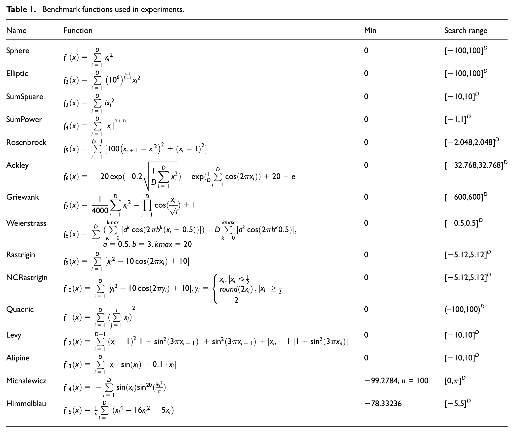
To make a fair comparison among PSO, AFSA, PSO-FSA, PSOEM-FSA and CIAFSA, these algorithms adopt the parameter settings in Table 2. Furthermore, all algorithms run 50 times independently and are stopped when the maximum number of 50,000 function evaluations (FEs) is reached (the population size is 50 and the maximum number of generations is 1000) in the cases of the low-, middle- and high-dimensional benchmark functions. The reported results are the best, the means and standard deviations of the statistical experimental data.

Table 2.

Parameters of the algorithms.

Algorithm	Parameter	Value
PSO	$ω$	[ 0.9, 0.4]
	$c_{1}$ , $c_{2}$	2
CIAFSA	$ξ_{t}$	0.5
PSOEM-FSA	$ξ_{t - 1}$	0.5
PSO-FSA	Visual_min	MaxD/100
	Step_min	MaxD/500
AFSA	Try_number	5
	$δ$	0.75

PSO, particle swarm optimization; AFSA, artificial fish swarm algorithm; CIAFSA, comprehensive improvement on the AFSA; PSOEM-FSA, the AFSA optimized by the PSO algorithm with extended memory; PSO-FSA, the AFSA optimized by PSO algorithm.

Optimization precision analysis

Tables 3 –5 show the best, the mean and the standard deviation of the results obtained by each algorithm under the budgeted FEs over 50 independent runs. In addition, the convergence curves of some benchmark functions are plotted in Figures 4 –6, where the abscissa represents FEs and the vertical axis represents the mean fitness, the value of which is respectively taken by log10.

Table 3.

Result comparisons of five algorithms on 10-dimensional benchmark functions f₁–f₁₃, 50-dimensional benchmark functions f₁₄ and f₁₅.

Function		f ₁	f ₂	f ₃	f ₄	f ₅
PSO	Best	2.1183e − 16	7.4850e + 00	2.7331e − 17	2.4203e − 11	1.7747e − 01
	Mean	3.8368e − 08	3.6207e + 03	1.0854e − 06	3.6816e − 08	3.5058e + 00
	SD	1.1046e − 07	4.2192e + 03	4.8525e − 06	1.0430e − 08	1.9290e + 00
AFSA	Best	1.5799e − 11	1.6055e − 07	3.7780e − 11	2.9407e − 14	5.6536e − 12
	Mean	1.2101e − 07	3.2876e − 02	8.4071e − 08	6.4669e − 12	4.2622e − 08
	SD	1.8393e − 07	6.5721e − 02	1.6023e − 07	1.3810e − 11	7.6992e − 08
PSO-FSA	Best	2.3588e − 07	1.1382e − 02	4.1681e − 08	1.6807e − 17	7.4357e − 11
	Mean	3.6647e − 01	2.0124e + 00	7.5472e − 02	1.9290e − 09	1.3446e − 08
	SD	7.2075e − 01	8.1085e + 00	2.7940e − 01	6.8209e − 09	2.6093e − 07
PSOEM-FSA	Best	6.1574e − 07	1.0290e − 02	5.2391e − 08	1.4275e − 15	1.2170e − 09
	Mean	4.2864e − 01	5.7295e + 00	5.4670e − 02	9.6959e − 10	1.8732e − 07
	SD	8.0407e − 01	1.0371e + 01	2.4446e − 01	1.6928e − 09	2.9746e − 07
CIAFSA	Best	1.0010e − 12	2.1820 + 01	9.7584e − 07	4.5703e − 13	2.5439e − 14
	Mean	6.5142e − 03	8.4034e + 03	4.7124e − 01	1.7204e − 09	1.4539e − 05
	SD	2.5897e − 03	3.5084e + 03	1.6089e + 00	3.4720e − 09	3.8146e − 05

Function		f ₆	f ₇	f ₈	f ₉	f ₁₀
PSO	Best	8.6074e − 06	1.1102e − 16	4.6635e + 00	1.7764e − 15	3.5527e − 15
	Mean	6.6523e − 01	8.1583e − 06	8.3310e + 00	1.9935e + 00	3.2000e + 00
	SD	5.9856e − 01	5.5708e − 05	1.4344e + 00	7.3343e + 00	7.7974e + 00
AFSA	Best	2.5014e − 04	2.4876e − 09	8.7228e − 03	3.1973e − 10	1.3769e − 10
	Mean	3.0884e − 02	7.1076e − 06	1.5537e − 01	2.3801e − 07	1.4520e − 07
	SD	1.9416e − 02	7.5721e − 05	8.4856e − 02	4.4421e − 07	3.5960e − 07
PSO-FSA	Best	5.9324e − 06	3.1972e − 08	7.2685e − 03	1.5313e − 08	3.4147e − 10
	Mean	1.2559e − 04	1.0278e − 01	2.7847e − 02	1.2158e − 06	1.1765e − 06
	SD	1.3162e − 04	1.5232e − 01	1.5109e − 02	1.8658e − 06	2.2431e − 06
PSOEM-FSA	Best	5.1294e − 07	2.9368e − 08	1.1590e − 02	3.0860e − 10	6.1640e − 11
	Mean	1.3177e − 04	1.0712e − 01	3.1737e − 02	8.3388e − 06	1.7111e − 06
	SD	1.2671e − 04	1.8437e − 01	1.0009e − 02	2.3974e − 05	3.4854e − 06
CIAFSA	Best	1.7901e − 06	7.4720e − 06	1.4784e − 03	4.5597e − 09	9.8588e − 12
	Mean	3.5575e − 04	1.5219e − 02	2.6870e − 02	2.0564e − 06	1.7612e − 07
	SD	3.9508e − 04	3.4673e − 01	1.4351e − 02	4.5475e − 06	6.9282e − 07

Function		f ₁₁	f ₁₂	f ₁₃	f ₁₄	f ₁₅
PSO	Best	3.3339e − 14	1.75289-03	9.1790e − 05	−25.8979	−60.397
	Mean	2.4670e − 05	1.4807e + 00	4.2387e − 01	−19.4491	−55.5206
	SD	1.3909e − 04	1.7036e + 00	5.3775e − 01	1.6658e + 00	2.2709e + 00
AFSA	Best	1.9810e − 08	1.3848e − 08	6.4112e − 08	−19.8925	−78.3323
	Mean	5.4407e − 05	2.3383e − 05	4.1416e − 06	−19.8921	−78.3323
	SD	1.2871e − 04	2.6305e − 05	3.6237e − 06	7.5097e − 04	2.9285e − 09
PSO-FSA	Best	1.1388e − 07	4.4483e − 07	5.5208e − 09	−20.5542	−78.3323
	Mean	1.6120e + 00	3.2021e − 06	7.1030e − 06	−19.9256	−78.3323
	SD	3.8659e + 00	2.4371e − 06	7.3669e − 06	1.4796e − 01	1.6244e − 10
PSOEM-FSA	Best	4.1076e − 06	4.7864e − 07	1.7445e − 07	−20.0552	−78.3323
	Mean	1.8184e + 00	6.8713e − 06	7.2759e − 06	−19.9006	−78.3323
	SD	3.9199e + 00	5.3888e − 06	8.5974e − 06	3.6412e − 02	1.1950e − 10
CIAFSA	Best	9.0400e − 05	1.9414e − 06	2.4285e − 06	−26.2018	−78.3323
	Mean	9.3433e + 00	8.9752e − 06	3.2583e − 05	−20.6346	−78.3323
	SD	2.1066e + 01	1.1835e − 05	2.4508e − 05	1.3953e − 04	8.4691e − 11

Abbreviations as in Table 2.

Table 4.

Result comparisons of five algorithms on 30-dimensional benchmark functions f_1–f13, 100-dimensional benchmark functions f₁₄ and f₁₅.

Function		f ₁	f ₂	f ₃	f ₄	f ₅
PSO	Best	1.4734e + 02	1.0096e + 06	3.9396e + 01	3.7076e − 11	3.4161e + 01
	Mean	6.3558e + 02	3.3264e + 06	8.2470e + 01	9.7781e − 08	5.8755e + 01
	SD	4.1107e + 02	1.8250e + 06	3.9077e + 01	9.9756e − 08	1.4691e + 01
AFSA	Best	4.2102e − 11	7.7441e − 06	7.1338e − 08	2.7045e − 13	3.9063e − 13
	Mean	6.7488e − 06	4.1811e − 01	2.7361e − 01	3.2420e − 11	9.3696e − 09
	SD	9.8753e − 06	9.5549e − 01	7.0887e − 01	7.0687e − 11	1.3756e − 08
PSO-FSA	Best	0	5.9855e − 05	1.5005e − 08	2.1995e − 16	1.8654e − 12
	Mean	1.1273e − 06	5.6249e − 02	1.5201e − 05	3.6775e − 12	1.3618e − 09
	SD	1.3107e − 06	9.9267e − 02	4.1582e − 05	1.2065e − 11	1.6820e − 09
PSOEM-FSA	Best	5.2180e − 12	6.8389e − 07	2.1428e − 10	4.7192e − 14	1.6994e − 11
	Mean	4.6360e − 07	1.1115e − 01	7.4587e − 08	3.6404e − 12	1.1804e − 09
	SD	9.8640e − 07	1.7860e − 01	1.5490e − 07	3.5784e − 12	1.6053e − 09
CIAFSA	Best	3.1727e − 16	3.9115e − 02	3.2790e − 12	2.8428e − 15	1.2878e − 15
	Mean	3.3597e − 08	2.0008e + 00	1.5609e − 08	9.1756e − 12	2.0949e − 08
	SD	9.8898e − 08	4.5206e + 00	2.5122e − 08	3.2652e − 11	6.5214e − 08

Function		f ₆	f ₇	f ₈	f ₉	f ₁₀
PSO	Best	1.0351e − 05	1.1102e − 16	3.7269e + 01	6.6407e − 03	5.5470e + 00
	Mean	8.4584e − 01	5.1944e − 06	4.0435e + 01	3.8177e + 01	6.0809e + 01
	SD	6.8172e − 01	2.3230e − 05	1.2113e + 00	2.7717e + 01	3.5086e + 01
AFSA	Best	3.5507e − 05	2.3099e − 09	6.3387e − 02	3.0293e − 09	4.8825e − 10
	Mean	6.0980e − 04	2.1825e − 05	1.4837e − 01	9.0062e − 08	4.1122e − 07
	SD	7.4656e − 04	3.9890e − 05	7.9504e − 02	1.4402e − 07	7.4987e − 07
PSO-FSA	Best	2.1296e − 05	1.6299e − 09	1.6016e − 02	1.2737e − 11	2.9358e − 10
	Mean	2.3202e − 04	1.4460e − 06	5.3924e − 02	3.4954e − 08	2.1094e − 07
	SD	2.6035e − 04	2.4769e − 06	3.7739e − 02	5.0460e − 08	4.5162e − 07
PSOEM-FSA	Best	2.4726e − 06	1.1683e − 10	1.4457e − 02	9.5134e − 09	1.6514e − 11
	Mean	1.1871e − 04	1.2548e − 06	5.8181e − 02	9.7812e − 06	1.8448e − 05
	SD	1.3370e − 04	3.6560e − 06	4.2526e − 02	1.2233e − 05	3.9378e − 05
CIAFSA	Best	3.7534e − 07	0	1.9190e − 03	1.7482e − 09	6.8372e − 11
	Mean	1.6245e − 04	6.5866e − 09	3.4394e − 02	6.8430e − 07	2.2245e − 07
	SD	2.3276e − 04	2.8071e − 08	2.3342e − 02	2.2684e − 06	4.1137e − 07

Function		f ₁₁	f ₁₂	f ₁₃	f ₁₄	f ₁₅
PSO	Best	9.2152e + 02	1.9372e + 01	3.9250e + 00	−41.47	−49.1823
	Mean	1.5473e + 03	4.8423e + 01	1.1329e + 01	−36.3557	−47.2507
	SD	4.9112e + 02	2.1222e + 01	4.2496e + 00	3.0092e + 00	1.2793e + 00
AFSA	Best	1.5314e − 07	2.0671e − 06	1.6129e − 06	−39.7847	−78.3323
	Mean	1.6541e − 03	4.1933e − 05	2.2718e − 05	−38.9807	−78.3323
	SD	2.1799e − 03	4.5220e − 05	2.1135e − 05	1.0805e + 00	8.7403e − 10
PSO-FSA	Best	1.6912e − 07	5.9139e − 07	2.3065e − 06	−41.8825	−78.3323
	Mean	2.2857e − 04	7.3049e − 06	1.2797e − 05	−40.1094	−78.3323
	SD	2.9015e − 04	6.0600e − 06	8.1033e − 06	5.2210e − 01	4.9453e − 10
PSOEM-FSA	Best	2.9224e − 07	3.5160e − 07	2.2575e − 07	−40.5472	−78.3323
	Mean	1.7114e − 04	1.2370e − 05	2.1263e − 05	−39.8189	−78.3323
	SD	3.2918e − 04	8.3940e − 06	3.3271e − 05	1.7163e − 01	6.0642e − 10
CIAFSA	Best	1.3234e − 05	1.3224e − 08	5.1581e − 08	−41.6213	−78.3323
	Mean	8.3256e − 04	1.1621e − 06	1.5394e − 06	−40.0724	−78.3323
	SD	7.7995e − 04	7.7914e − 07	1.3026e − 06	1.5440e − 01	1.9233e − 10

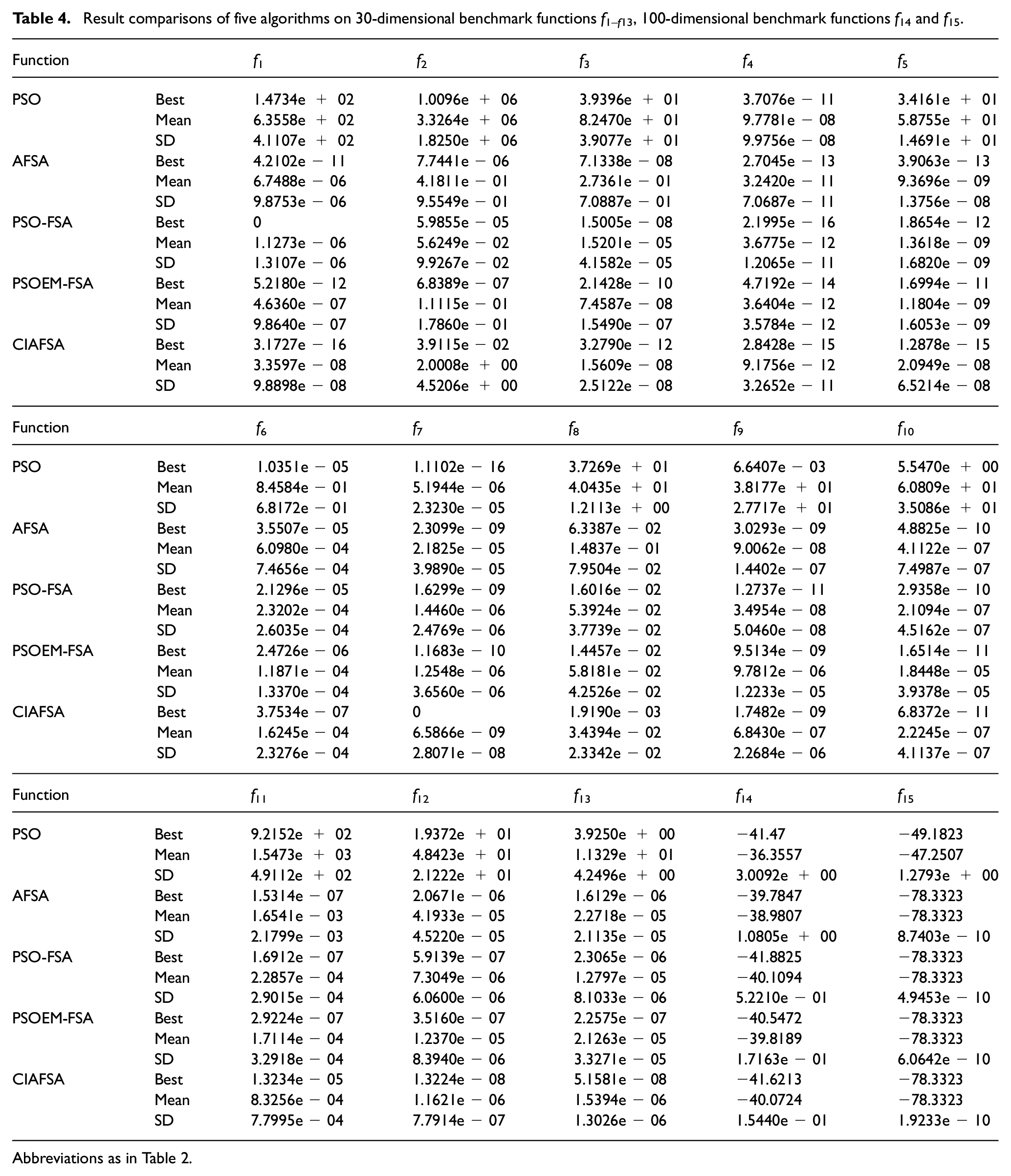
Abbreviations as in Table 2.

Table 5.

Result comparisons of five algorithms on 60-dimensional benchmark functions f₁–f₁₃, 200-dimensional benchmark functions f₁₄ and f₁₅.

Function		f ₁	f ₂	f ₃	f ₄	f ₅
PSO	Best	2.5741e + 03	2.0554e + 07	6.0384e + 02	3.3703e − 10	1.6711e + 00
	Mean	4.2037e + 03	3.7801e + 07	1.0909e + 03	9.6037e − 08	2.0078e + 02
	SD	9.7034e + 02	1.3952e + 07	2.8861e + 02	2.1252e − 07	8.9242e + 01
AFSA	Best	1.3930e − 10	5.3094e − 04	2.1686e − 06	6.6908e − 15	2.9077e − 12
	Mean	2.4935e − 05	1.5971e + 00	2.6475e − 01	4.7713e − 11	8.1679e − 06
	SD	4.2693e − 05	3.5257e + 00	5.7892e − 01	6.9521e − 11	1.4586e − 05
PSO-FSA	Best	2.8724e − 10	1.3299e − 04	4.6270e − 09	3.9070e − 19	1.3884e − 13
	Mean	2.5736e − 06	3.6920e − 01	1.5746e − 06	6.3973e − 12	2.9827e − 09
	SD	4.7670e − 06	8.6628e − 01	2.7154e − 06	1.0558e − 11	1.3447e − 08
PSOEM-FSA	Best	5.3492e − 10	4.6051e − 04	9.5161e − 09	7.5160e − 15	1.0085e − 12
	Mean	1.8649e − 06	2.6562e − 01	1.8444e − 06	8.6518e − 12	3.1231e − 09
	SD	3.5060e − 06	4.9935e − 01	2.4187e − 06	1.1025e − 11	9.4296e − 09
CIAFSA	Best	0	4.9665e − 07	1.2559e − 08	2.8954e − 16	1.9802e − 14
	Mean	5.1510e − 08	1.9624e − 03	1.9108e − 06	3.3259e − 14	2.3955e − 09
	SD	1.6368e − 07	3.8799e − 03	3.9537e − 06	6.6855e − 14	6.6315e − 09

Function		f ₆	f ₇	f ₈	f ₉	f ₁₀
PSO	Best	9.6591e + 00	1.1102e − 016	8.7499e + 01	4.3408e + 01	3.8070e + 01
	Mean	1.1218e + 01	9.0136e + 00	9.225e + 01	1.5217e + 02	1.4656e + 02
	SD	9.3009e − 01	2.7743e + 01	2.3542e + 00	6.4118e + 01	5.0314e + 01
AFSA	Best	8.7200e − 07	1.5964e − 09	8.4760e − 04	2.3377e − 09	6.5391e − 09
	Mean	1.7513e − 03	2.4039e − 05	1.9546e − 01	5.5039e − 07	6.8894e − 07
	SD	5.8452e − 03	5.4480e − 05	2.0196e − 01	8.8707e − 07	7.1208e − 07
PSO-FSA	Best	1.3503e − 05	2.8587e − 09	1.4438e − 01	2.4237e − 10	1.0658e − 13
	Mean	1.9175e − 04	2.7320e − 06	2.9279e − 01	1.1397e − 08	1.1369e − 07
	SD	1.9348-04	4.8729e − 06	1.0316e − 01	2.7316e − 08	1.4725e − 07
PSOEM-FSA	Best	3.8073e − 07	2.8690e − 10	3.5696e − 02	4.0501e − 12	4.3957e − 08
	Mean	2.0146e − 04	2.3149e − 06	2.3734e − 01	1.8252e − 05	6.6718e − 06
	SD	1.6315e − 04	2.6252e − 06	1.5504e − 01	3.3357e − 05	9.6918e − 06
CIAFSA	Best	6.4733e − 07	0	2.7028e − 02	8.5265e − 13	2.5175e − 10
	Mean	1.3092e − 05	0	7.2490e − 02	2.9154e − 06	1.6846e − 06
	SD	1.2073e − 05	0	4.7980e − 02	5.2509e − 06	3.0213e − 06

Function		f ₁₁	f ₁₂	f ₁₃	f ₁₄	f ₁₅
PSO	Best	5.6245e + 03	1.2016e + 02	2.0665 + 00	−67.7555	−42.8697
	Mean	8.8285e + 03	1.9065e + 02	3.2824e + 01	−62.1173	−41.0378
	SD	2.1603e + 03	4.2909e + 01	6.2027e + 00	2.8125e + 00	1.0119e + 00
AFSA	Best	2.4419e − 05	3.7358e − 06	5.8474e − 06	−79.5693	−78.3323
	Mean	2.8879e − 02	5.5957e − 05	9.2802e − 05	−79.5238	−78.3323
	SD	8.3620e − 02	4.5659e − 05	7.8536e − 05	6.6629e − 02	2.9760e − 09
PSO-FSA	Best	4.4900e − 08	3.3989e − 06	3.1541e − 07	−79.5692	−78.3323
	Mean	3.9554e − 03	2.2132e − 05	1.5973e − 05	−79.52	−78.3323
	SD	7.2107e − 03	1.6118e − 05	1.1125e − 05	7.4320e − 02	4.5118e − 10
PSOEM-FSA	Best	1.8260e − 06	1.2959e − 06	1.1584e − 06	−79.5693	−78.3323
	Mean	6.7912e − 03	1.5060e − 05	1.4080e − 05	−79.4369	−78.3323
	SD	1.3759e − 02	1.1628e − 05	1.3926e − 05	2.7556e − 01	1.3840e − 10
CIAFSA	Best	1.6932e − 08	1.4469e − 08	1.0777e − 09	−79.5692	−78.3323
	Mean	2.8163e − 05	1.3262e − 06	3.8972e − 06	−79.3662	−78.3323
	SD	5.3152e − 05	1.1843e − 06	3.3664e − 06	2.8534e − 01	1.2235e − 10

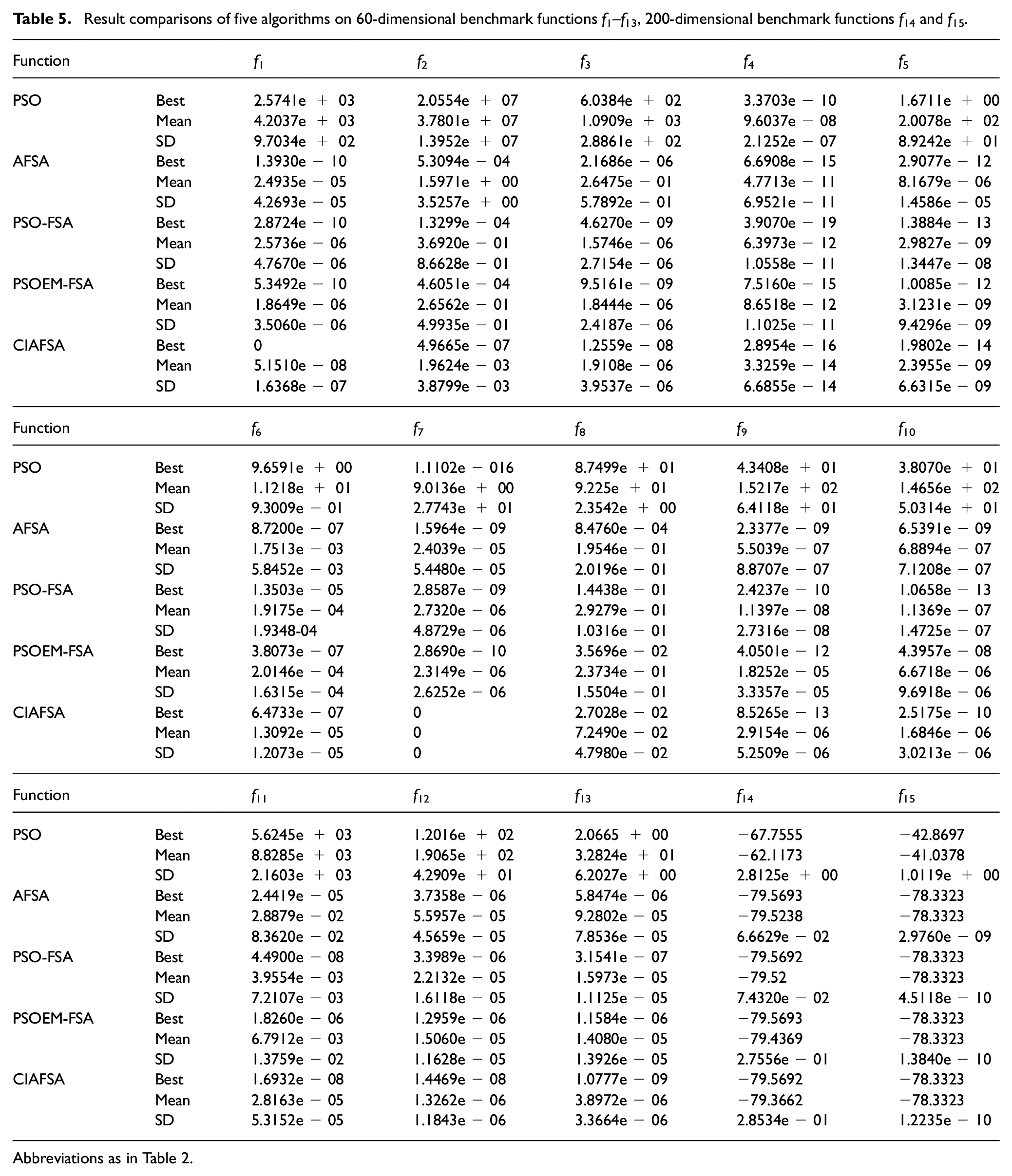
Abbreviations as in Table 2.

Figure 4.

Convergence characteristics of the five different algorithms on 10-dimensional test functions: (a) f₁; (b) f₅; (c) f₆; (d) f₇; (e) f₉; (f) f₁₀; (g) f₁₂; (h) f₁₃.

Figure 5.

Convergence characteristics of the five different algorithms on 30-dimensional test functions: (a) f₁; (b) f₅; (c) f₆; (d) f₇; (e) f₉; (f) f₁₀; (g) f₁₂; (h) f₁₃.

Figure 6.

Convergence characteristics of the five different algorithms on 60-dimensional test functions: (a) f₁; (b) f₅; (c) f₆; (d) f₇; (e) f₉; (f) f₁₀; (g) f₁₂; (h) f₁₃.

Some insightful conclusions can be drawn from Tables 3 –5. CIAFSA performs significantly better than the other compared algorithms on most cases. For the low-dimensional functions in Table 3, the means and standard deviations of the results obtained by CIAFSA are significantly better than PSO, AFSA, PSO-FSA and PSOEM-FSA on 6, 8, 14 and 15 cases, respectively, whereas only PSO surpass CIAFSA on 1, 3, 7 and 11 cases. From the results of the middle-dimensional functions in Table 4, it is clear that CIAFSA consistently outperforms the other compared methods in the majority of the test functions. CIAFSA significantly exceeds PSO, AFSA, PSO-FSA and PSOEM-FSA on 1, 2, 3, 7, 10, 12 and 13 cases, respectively, whereas CIAFSA cannot lose the superiority on all the cases. Differently from the results of the low-dimensional functions, CIAFSA obviously overcomes PSO on any case. From Table 5, similarly to the results of the middle-dimensional functions, CIAFSA also overcomes the other algorithms on most cases. Thus, CIAFSA performs significantly better than PSO, AFSA, PSO-FSA and PSOEM-FSA on 1, 2, 4, 6, 7, 11, 12 and 15 cases, respectively. For the remaining cases, they perform the same, whereas CIAFSA improves the robustness in performance on most cases.

Furthermore, by comparing with Tables 3 –5, it can be seen that the results obtained by CIAFSA in cases of the high-dimensional functions are better than the results obtained by CIAFSA in cases of the low- and middle-dimensional functions on most cases. To describe the advantage of CIAFSA vividly, the convergence graphs of some benchmark functions are plotted in Figures 4 –6. It can be observed from Tables 3 –5 and Figures 4 –6 that CIAFSA exhibits higher convergence accuracy than PSO, AFSA, PSO-FSA and PSOEM-FSA on all cases. In particular, the curves shown in Figures 4 –6 demonstrate that CIAFSA has higher reliability and robustness on most multimodal test functions in the cases of the middle and high dimension. This is because CIAFSA may combine the exploration capabilities of the PSOEM and the adaptive exploitation capabilities of the AFSA with adaptive visual and step, which performs an ideal balance between the exploration and the exploitation.

Volatility analysis of optimal results

To measure the merits of the algorithm performance, one of the criteria is to find the optimal value with the desired precision. After five algorithms ran 100 times independently, we obtained the standard deviations of 100 optimization results of the five algorithms. Moreover, the standard deviations are used to reflect and compare the performance of four algorithms, and are shown in Table 6 and Figure 8.

Table 6.

Standard deviations of optimization results of five algorithms on eight benchmark functions with D = 30.

Function	Algorithm
	PSO	AFSA	PSO-FSA	PSOEM-FSA	CIAFSA
f ₁	1.2065e + 02	4.1582e − 06	1.5784e − 06	2.0949e − 07	3.7739e − 08
f ₅	2.1825e + 01	1.1102e − 08	4.7110e − 09	2.1094e − 09	2.2190e − 09
f ₆	3.7732e − 01	5.4402e − 04	4.5162e − 04	2.6941e − 04	2.4508e − 04
f ₇	7.7441e − 05	3.6404e − 05	3.4954e − 06	3.5086e − 06	6.8172e − 08
f ₉	1.6245e + 01	1.2540e − 07	3.5507e − 08	2.1825e − 05	3.3597e − 07
f ₁₀	2.2857e + 01	4.1107e − 07	2.1273e − 07	3.6775e − 05	1.1804e − 07
f ₁₂	5.3924e + 01	4.1582e − 05	4.6270e − 06	2.0146e − 06	1.9108e − 07
f ₁₃	1.8444e + 00	5.4480e − 05	9.6918e − 06	4.8729e − 05	2.8870e − 06

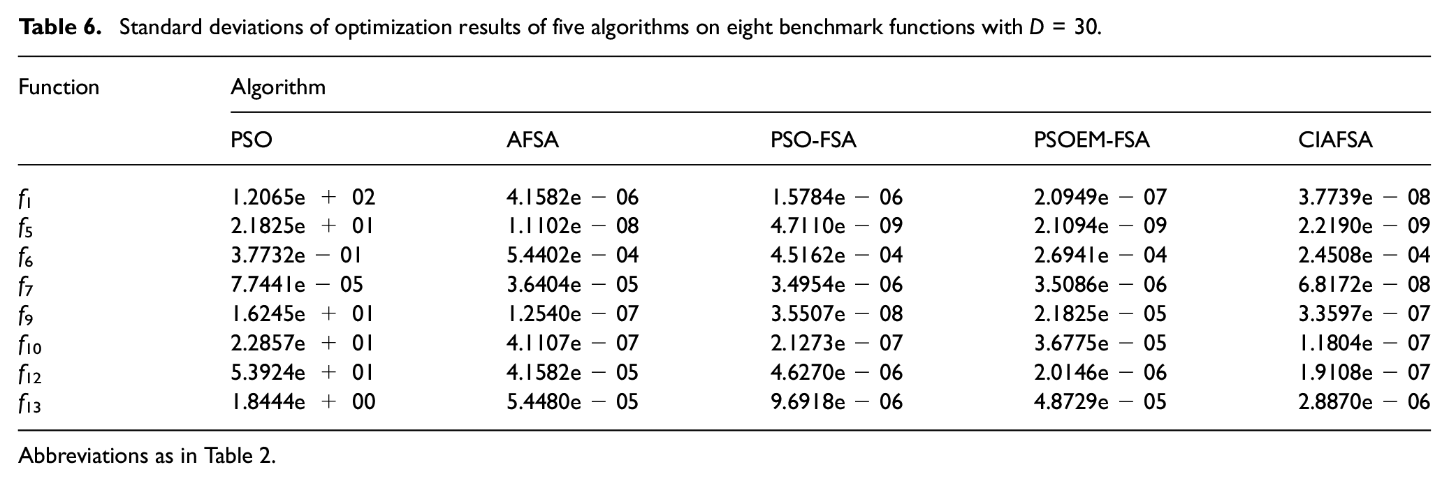
Abbreviations as in Table 2.

From Table 6 and Figure 7, it can be seen that the standard deviations obtained by CIAFSA outperform the other compared methods in the majority of the test functions, indicating that the fluctuation of the optimization results of CIAFSA is the smallest, and this algorithm can guarantee a higher accuracy on most cases, whereas only AFSA and PSO-FSA weakly overcome CIAFSA on f₉. For the remaining cases, CIAFSA improves the performance effectiveness.

Figure 7.

Standard deviations of optimization results of five algorithms.

Algorithm time complexity analysis

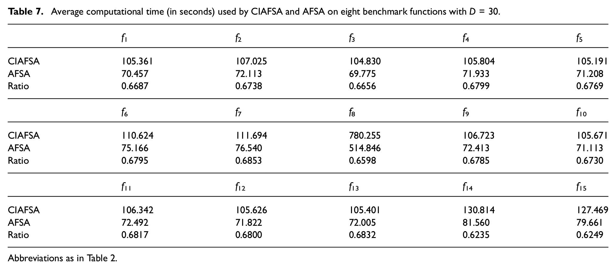
Algorithm complexity is another standard for measuring the merits of an algorithm. Here, we compare the average runtime between CIAFSA and the original AFSA. The convergence precision of the Weierstrass function is set to 1e-2 and the convergence precisions of the other functions is set to 1e-3. All algorithms ran 100 times independently and the average computational time these algorithms demand to achieve the predetermined convergence precision is shown in Table 7.

Table 7.

Average computational time (in seconds) used by CIAFSA and AFSA on eight benchmark functions with D = 30.

	f ₁	f ₂	f ₃	f ₄	f ₅
CIAFSA	105.361	107.025	104.830	105.804	105.191
AFSA	70.457	72.113	69.775	71.933	71.208
Ratio	0.6687	0.6738	0.6656	0.6799	0.6769

	f ₆	f ₇	f ₈	f ₉	f ₁₀
CIAFSA	110.624	111.694	780.255	106.723	105.671
AFSA	75.166	76.540	514.846	72.413	71.113
Ratio	0.6795	0.6853	0.6598	0.6785	0.6730

	f ₁₁	f ₁₂	f ₁₃	f ₁₄	f ₁₅
CIAFSA	106.342	105.626	105.401	130.814	127.469
AFSA	72.492	71.822	72.005	81.560	79.661
Ratio	0.6817	0.6800	0.6832	0.6235	0.6249

Abbreviations as in Table 2.

We can conclude from Table 7 that CIAFSA has an additional computation burden compared with the original AFSA, as discussed in the time complexity analysis. The ratio that is the value of the cost of the original AFSA divided by that of the CIAFSA is also reported in the table. Based on the Table 7, it can be concluded that the runtime of CIAFSA mainly comes from the function evaluation.

Experiments of PV modules in series under PS conditions

Taking 10 PV modules in series as an example, when the entire modules are in an environment at 25°C and irradiance levels of 1000 W/m², the output power–voltage characteristic curve is shown in Figure 8. However, when they are at a temperature of 25°C and irradiance levels 100, 200, 300, 400, 500, 600, 700, 800, 900 and 1000 W/m², the output power–voltage characteristic curve is shown in Figure 9. Figure 9 shows that the characteristic curve appears to be 10 peaks. Obviously, the existence of local minima will lead to failure of the conventional algorithm for MPPT.

Figure 8.

Output characteristics under illumination conditions.

Figure 9.

Output characteristics under partial shading (PS) conditions.

The proposed algorithm for MPPT under PS conditions

In the simulation process, it is assumed that the environmental temperature remains at 25°C. The short circuit current of the arrays described by Equation (13) at T = 25°C and Sun≤1000 W/m² is no more than 4 A, so the optimal range of the algorithm is set to [0, 5]. In addition, the fish scale is set to 5, the number of iterations is set to 10, the value of the MaxD should be set to 4, the values of ξ_t and ξ_t − 1 are separately set to 0.5 and 0.5 (Duan et al., 2011), and other parameters are shown in Table 2.

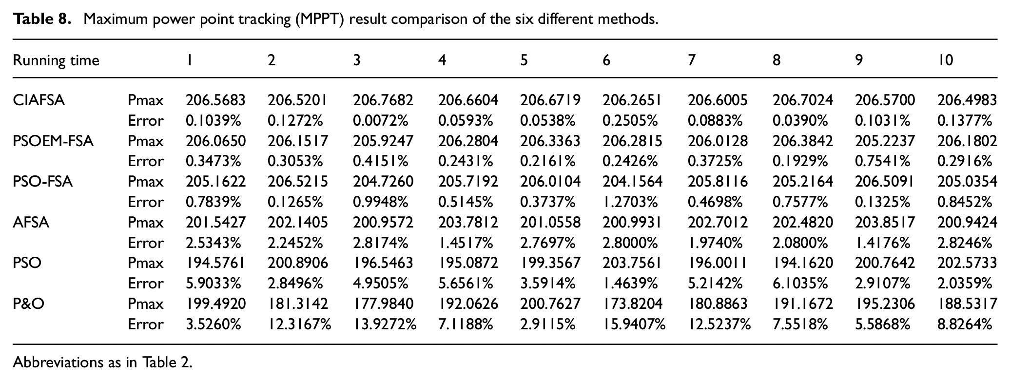
The algorithms independently ran 10 times and the results are shown in Table 8. In addition, the P&O method in engineering is also used in the environment for comparison with CIAFSA. The short circuit current of the arrays described by the formula (13) at T = 25°C and Sun≤1000 W/m² was no more than 4 A, so the working point current of disturbance observation was randomly initialized within the range of [1.5, 2.5] to simulate the working point of the PV system before the PS conditions appeared. The perturbation step length of the P&O method is set to 0.05 and the number of iterations is set to 50.

Table 8.

Maximum power point tracking (MPPT) result comparison of the six different methods.

Running time		1	2	3	4	5	6	7	8	9	10
CIAFSA	Pmax	206.5683	206.5201	206.7682	206.6604	206.6719	206.2651	206.6005	206.7024	206.5700	206.4983
CIAFSA	Error	0.1039%	0.1272%	0.0072%	0.0593%	0.0538%	0.2505%	0.0883%	0.0390%	0.1031%	0.1377%
PSOEM-FSA	Pmax	206.0650	206.1517	205.9247	206.2804	206.3363	206.2815	206.0128	206.3842	205.2237	206.1802
PSOEM-FSA	Error	0.3473%	0.3053%	0.4151%	0.2431%	0.2161%	0.2426%	0.3725%	0.1929%	0.7541%	0.2916%
PSO-FSA	Pmax	205.1622	206.5215	204.7260	205.7192	206.0104	204.1564	205.8116	205.2164	206.5091	205.0354
PSO-FSA	Error	0.7839%	0.1265%	0.9948%	0.5145%	0.3737%	1.2703%	0.4698%	0.7577%	0.1325%	0.8452%
AFSA	Pmax	201.5427	202.1405	200.9572	203.7812	201.0558	200.9931	202.7012	202.4820	203.8517	200.9424
AFSA	Error	2.5343%	2.2452%	2.8174%	1.4517%	2.7697%	2.8000%	1.9740%	2.0800%	1.4176%	2.8246%
PSO	Pmax	194.5761	200.8906	196.5463	195.0872	199.3567	203.7561	196.0011	194.1620	200.7642	202.5733
PSO	Error	5.9033%	2.8496%	4.9505%	5.6561%	3.5914%	1.4639%	5.2142%	6.1035%	2.9107%	2.0359%
P&O	Pmax	199.4920	181.3142	177.9840	192.0626	200.7627	173.8204	180.8863	191.1672	195.2306	188.5317
P&O	Error	3.5260%	12.3167%	13.9272%	7.1188%	2.9115%	15.9407%	12.5237%	7.5518%	5.5868%	8.8264%

Abbreviations as in Table 2.

It can be deduced from Table 8 that the CIAFSA method can catch the MPP with higher precision and more power output than the other five methods, whereas only the PSOEM-FSA method and the PSO-FSA method overcame the proposed method on the sixth and the second operations, respectively. For the remaining cases, the CIAFSA method improves the robustness and effectiveness of the performance. To sum up, CIAFSA obviously improves the reliability and effectiveness of MPPT for the PV system under PS conditions.

Simulation analysis on the experimental platform

The above described control algorithm was applied to control the PV system. The simulation model of PV array is made of two PV modules, which are connected in series. The block diagram of the MPPT system (Veerachary et al., 2002) is shown in Figure 10.

Figure 10.

Photovoltaic (PV) array with maximum power point tracking (MPPT) schematic of the experimental modelling and control scheme.

In order to make comparison of the simulation easier, a boost control circuit adopts the resistance as the load. The MPPT controller respectively adopts the CIAFSA, PSOEM-FSA, PSO-FSA and the traditional point-by-point comparison methods to drive the boost control circuit. In this paper, the shading conditions are divided into two cases, including: Case 1, setting G₁ = 1000 W/m², G₂ = 700 W/m², where the environment temperature is T = 25°C; Case 2, setting G₁ = 1000 W/m², G₂ = 500 W/m², where the environment temperature is T = 25°C. The parameters in simulation are as follows: the boost inductor L = 6.6 mH, the filter capacitor C₁ = 82 μF, the capacitor of the DC bus C₂ = 47 μF and load R = 40 Ω.

Results and discussion

In order to test the effectiveness of the CIAFSA method, this method is compared with the PSOEM-FSA, PSO-FSA and the traditional point-by-point comparison methods in the different shading situations. Results and comparative analysis are as follows.

Case 1: G₁ = 1000 W/m² and G₂ = 700 W/m²

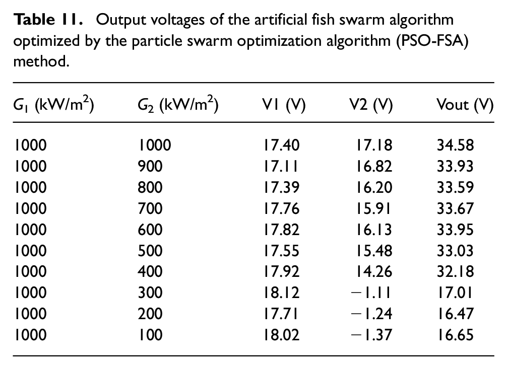
System voltages at different shading conditions, adopting the four methods, are plotted in Figures 11 –14, respectively, where the abscissa represents the time and the vertical axis represents the voltage values. In Figures 11 –14, Vout represents the total voltage value of the two PV modules, V1 represents the output voltage value when the irradiance of the PV module (G₁) is 1000 W/m² and V2 represents the output voltage value when the irradiance of the other module (G₂) is 700 W/m². Furthermore, Tables 9 –12 shows the output voltage values of the four methods when G₁ remains at 1000 W/m² and G₂ changes from 1000 to 100 W/m².

Figure 11.

System voltages tested on the comprehensive improvement on the artificial fish swarm algorithm (CIAFSA) method at different shading conditions (G₁ = 1000 W/m² and G₂ = 700 W/m²).

Figure 12.

System voltages tested on the artificial fish swarm algorithm optimized by particle swarm optimization algorithm with extended memory (PSOEM-FSA) method at different shading conditions (G₁ = 1000 W/m² and G₂ = 700 W/m²).

Figure 13.

System voltages tested on the artificial fish swarm algorithm optimized by particle swarm optimization algorithm (PSO-FSA) method at different shading conditions (G₁ = 1000 W/m² and G₂ = 700 W/m²).

Figure 14.

System voltages tested on the traditional point-by-point comparison method at different shading conditions (G₁ = 1000 W/m² and G₂ = 700 W/m²).

Table 9.

Output voltages of the comprehensive improvement on the artificial fish swarm algorithm (CIAFSA) method.

G₁ (kW/m²)	G₂ (kW/m²)	V1 (V)	V2 (V)	Vout (V)
1000	1000	18.26	18.25	36.51
1000	900	18.20	18.16	36.36
1000	800	18.24	18.11	36.35
1000	700	18.19	18.03	36.22
1000	600	18.25	17.95	36.20
1000	500	18.25	17.73	35.98
1000	400	18.26	17.71	35.97
1000	300	18.17	17.60	35.77
1000	200	18.24	17.52	35.76
1000	100	18.20	16.01	34.21

Table 10.

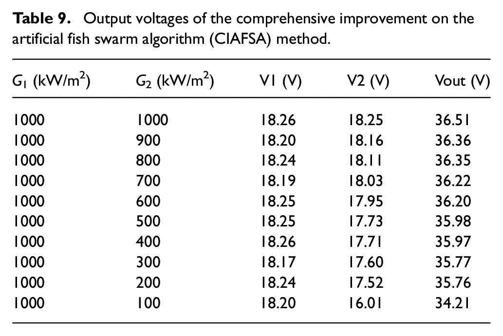
Output voltages of the the artificial fish swarm algorithm optimized by the particle swarm optimization algorithm with extended memory (PSOEM-FSA) method.

G₁ (kW/m²)	G₂ (kW/m²)	V1 (V)	V2 (V)	Vout (V)
1000	1000	18.21	18.13	36.34
1000	900	18.24	18.02	36.26
1000	800	18.19	17.98	36.17
1000	700	18.32	17.94	36.26
1000	600	18.26	17.83	36.09
1000	500	18.25	17.65	35.90
1000	400	18.18	17.60	35.78
1000	300	18.20	17.58	35.78
1000	200	18.23	16.78	35.01
1000	100	18.13	15.31	33.44

Table 11.

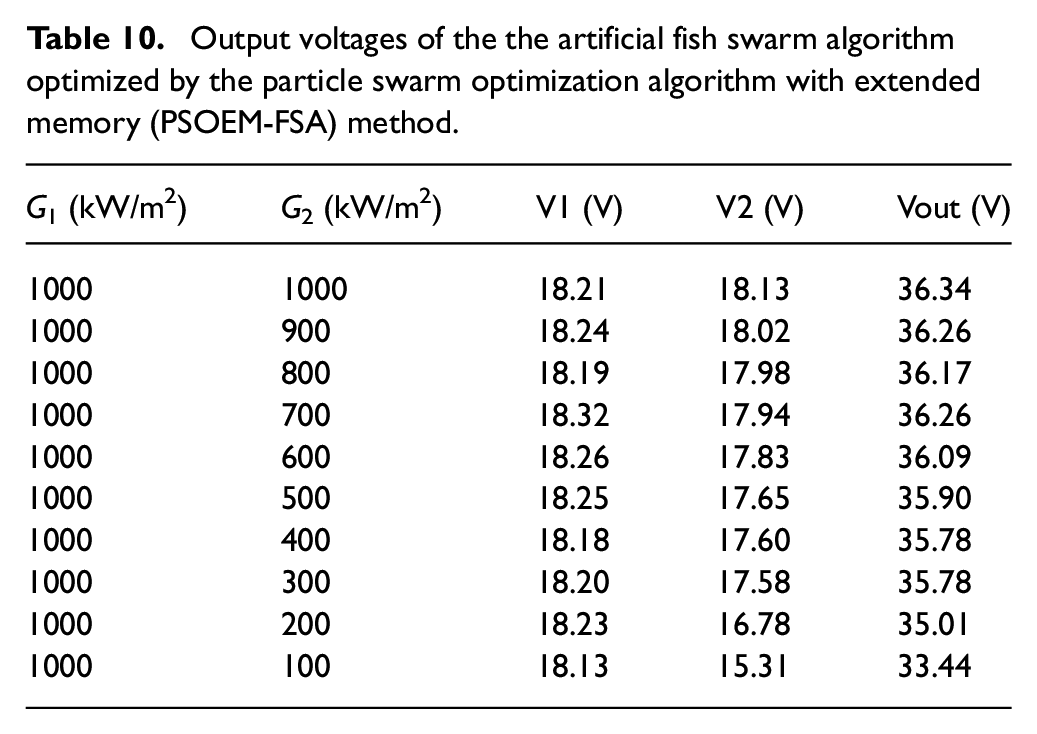
Output voltages of the artificial fish swarm algorithm optimized by the particle swarm optimization algorithm (PSO-FSA) method.

G₁ (kW/m²)	G₂ (kW/m²)	V1 (V)	V2 (V)	Vout (V)
1000	1000	17.40	17.18	34.58
1000	900	17.11	16.82	33.93
1000	800	17.39	16.20	33.59
1000	700	17.76	15.91	33.67
1000	600	17.82	16.13	33.95
1000	500	17.55	15.48	33.03
1000	400	17.92	14.26	32.18
1000	300	18.12	−1.11	17.01
1000	200	17.71	−1.24	16.47
1000	100	18.02	−1.37	16.65

Table 12.

Output voltages of the traditional point-by-point comparison method.

G₁ (kW/m²)	G₂ (kW/m²)	V1 (V)	V2 (V)	Vout (V)
1000	1000	18.18	17.68	35.86
1000	900	17.94	17.25	35.19
1000	800	17.30	16.01	33.31
1000	700	16.55	15.33	31.88
1000	600	17.42	15.89	33.31
1000	500	17.98	15.38	33.36
1000	400	18.01	16.01	34.02
1000	300	16.78	−2.02	14.76
1000	200	17.68	−2.15	15.53
1000	100	18.07	−2.33	15.74

It can be observed from Figures 11 –13 and Tables 9 –11 that CIAFSA consistently outperforms the PSOEM-FSA method and the PSO-FSA method on the stability of the output voltages in most cases. From Figures 11 –14 and Tables 9 –12, it is also clear that the voltage values tested on the traditional point-by-point comparison method are more stable, but the voltage average values tested on the CIAFSA method are more than the values tested on the other methods.

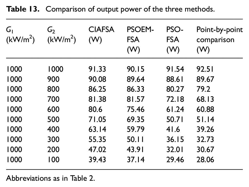
Furthermore, Figure 15 shows the output power curves of the three methods. From Figure 15, it can be seen that the proposed method consistently outperforms the PSOEM-FSA, the PSO-FSA and the traditional point-by-point comparison methods in the first stage (t = 0 to t = 0.02). In the second stage (t = 0.02 to t = 0.04), although the traditional point-by-point comparison method outperforms the other three methods on the stability of the output power, the proposed method obviously improves the output power of the PV array when compared with the other three methods.

Figure 15.

Output power curves of the three methods.

Table 13 shows the output power values of the four methods when G₁ remains at 1000 W/m² and G₂ changes from 1000 to 100 W/m². We can conclude from Table 13 that the CIAFSA method consistently outperforms the other three methods on the stability of the output power when the PV array is under various PS conditions.

Table 13.

Comparison of output power of the three methods.

G₁ (kW/m²)	G₂ (kW/m²)	CIAFSA (W)	PSOEM-FSA (W)	PSO-FSA (W)	Point-by-point comparison (W)
1000	1000	91.33	90.15	91.54	92.51
1000	900	90.08	89.64	88.61	89.67
1000	800	86.25	86.33	80.27	79.2
1000	700	81.38	81.57	72.18	68.13
1000	600	80.6	75.46	61.24	60.88
1000	500	71.05	69.35	50.71	51.14
1000	400	63.14	59.79	41.6	39.26
1000	300	55.35	50.11	36.15	32.73
1000	200	47.02	43.91	32.01	30.67
1000	100	39.43	37.14	29.46	28.06

Abbreviations as in Table 2.

Case 2: G₁ = 1000 W/m² and G₂ = 500 W/m²

System voltages at different shading conditions by adopting the four methods are plotted in Figures 16 –19 respectively, where the abscissa represents the time and the vertical axis represents the voltage values. In Figures 16 –19, Vout represents the total voltage value of the two PV modules, V1 represents the voltage value when the irradiance of the PV module (G₁) is 1000 W/m² and V2 represents the voltage value when the irradiance of the other module (G₂) is 500 W/m².

Figure 16.

System voltages tested on the comprehensive improvement on the artificial fish swarm algorithm (CIAFSA) method at different shading conditions (G₁ = 1000 W/m² and G₂ = 500 W/m²).

Figure 17.

Figure 18.

Figure 19.

System voltages tested on the traditional point-by-point comparison method at different shading conditions (G₁ = 1000 W/m² and G₂ = 500 W/m²).

It can be observed from Figures 16 –18 that the proposed method consistently outperforms the PSOEM-FSA method and the PSO-FSA method on the stability of the output voltages in most cases. From Figures 16 –19, similarly to the results of the Case 1, although the voltage values tested on the traditional point-by-point comparison method are more stable, CIAFSA also overcomes the other algorithms in most cases.

Furthermore, it can be seen from Figure 20 that the CIAFSA method consistently outperforms the PSOEM-FSA, the PSO-FSA and the traditional point-by-point comparison methods in the first stage (t = 0 to t = 0.015). In the second stage (t = 0.015 to t = 0.04), although the traditional point-by-point comparison method outperforms the other three methods on the stability of the output power, the CIAFSA method obviously improves the output power of the PV array when compared with the other three methods. In addition, similarly to the results of the Case 1, some insightful conclusions can be drawn from Figure 20: the CIAFSA method consistently outperforms the other three methods on the stability of the output power when the PV array is under various PS conditions.

Figure 20.

Output power curves of the three methods.

Conclusions

In this paper, a new intelligent algorithm called CIAFSA is proposed and applied to MPPT of the PV system under PS. Finally, various tracking simulation tests have been performed and the four control methods were applied to control the PV system on the experimental platform to verify the effectiveness of the proposed MPPT method. Experimental results show that the CIAFSA method can easily avoid the constraint of multiple local extreme value points and catch the MPP of the current environment with high precision. Compared with the other methods, the proposed method obviously improves the reliability and effectiveness of MPPT for the PV system under PS conditions. In future work, we will conduct more experiments to verify whether the extended memory factor (ξ_t − 1) can be set according to a non-uniform degree of PS conditions to improve the reliability and effectiveness of MPPT under PS further.

Footnotes

Declaration of conflicting interest

The authors declare that there is no conflict of interest.

Funding

This work has been supported by the National Natural Science Foundation of China (Grant No. 51377187), the Graduate Scientific Research and Innovation Foundation of Chongqing (Grant No. CYB16048) and the China Scholarship Council (CSC).

References

Alajmi

Ahmed

Finney

et al . (2011) Fuzzy-logic-control approach of a modified hill-climbing method for maximum power in micro grid standalone PV systems. IEEE Transactions on Power Electronics26(4): 1022–1030.

Banks

Vincent

Anyakoha

(2007) A review of particle swarm optimization. Part I: background and development. Natural Computing6(4): 467–484.

Bendib

Krim

Belmili

et al . (2014) An intelligent MPPT approach based on neural-network voltage estimator and fuzzy controller, applied to a stand-alone PV system. In: Proceedings of the IEEE 23rd International Symposium on Industrial Electronics (ISIE), pp. 404–409.

Bing

Wen

(2010) Scheduling arrival aircrafts on multi-runway based on an improved artificial fish swarm algorithm. In: Proceedings of the International Conference on Computer and Information Science, pp. 499–502.

Carannante

Fraddanno

Pagano

et al . (2009) Experimental performance of MPPT algorithm for photovoltaic sources subject to inhomogeneous insolation. IEEE Transactions on Industrial Electronics56(11): 4374–4380.

Duan

Huang

Lei

et al . (2011) Simulation analysis of particle swarm optimization algorithm with extended memory. Control and Decision26(7): 1087–1100.

Duan

Mao

Duan

et al . (2016) An improved artificial fish swarm algorithm optimized by particle swarm optimization algorithm with extended memory. Kybernetes45(2): 210–222.

Eberhart

Kennedy

(1995) A new optimizer using particle swarm theory. In: Proceedings of the International Symposium on Micro-Machines and Human Science, pp. 39–43.

Eusuff

Lansey

(2003) Optimization of water distribution network design using the shuffled frog leaping algorithm. Journal of Water Resources Planning and Management129: 210–225.

10.

Femia

Petrone

Spagnuolo

et al . (2005) Optimization of perturb and observe maximum power point tracking method. IEEE Transactions on Power Electronics20(4): 963–973.

11.

Gülcü

Kodaz

(2015) A novel parallel multi-swarm algorithm based on comprehensive learning particle swarm optimization. Engineering Applications of Artificial Intelligence45: 33–45.

12.

Huang

Chen

(2013) An improved artificial fish swarm algorithm based on hybrid behavior selection. International Journal of Control and Automation6(5): 103–116.

13.

Ishaque

Salam

Amjad

et al . (2012) An improved particle swarm optimization (PSO)–based MPPT for PV with reduced steady-state oscillation. IEEE Transactions on Power Electronics27(8): 3627–3638.

14.

Y-H

Jung

D-Y

Kim

J-G

et al . (2011) A real maximum power point tracking method for mismatching compensation in PV array under partially shaded conditions. IEEE Transactions on Power Electronics26(4): 1001–1009.

15.

Kadri

Gaubert

Champenois

(2011) An improved maximum power point tracking for photovoltaic grid-connected inverter based on voltage-oriented control. IEEE Transactions on Industrial Electronics58(1): 66–75.

16.

Karaboga

(2005) An idea based on honey bee swarm for numerical optimization. Technical Report—TR06. Erciyes University.

17.

Lei

Seem

(2011) Sequential ESC-based global MPPT control for photovoltaic array with variable shading. IEEE Transactions on Sustainable Energy2(3): 348–358.

18.

Shao

Qian

(2002) An optimizing method based on autonomous animats: fish-swarm algorithm. Systems Engineering – Theory & Practice22(11): 32–38.

19.

Liu

Duan

Cai

(2011) Photovoltaic DC-building-module based BIPV system-concept and design considerations. IEEE Transactions on Power Electronics26(5): 1418–1429.

20.

Luo

Wei

Wang

(2010) The optimization of PID controller parameters based on an improved artificial fish swarm algorithm. In: Proceedings of the International Workshop on Advanced Computational Intelligence, pp. 328–332.

21.

Ngan

Tan

(2016) Photovoltaic multiple peaks power tracking using particle swarm optimization with artificial neural network algorithm. Advances in Solar Photovoltaic Power Plants, pp. 107–138.

22.

Patel

Agarwal

(2008) Maximum power point tracking scheme for PV systems operating under partially shaded conditions. IEEE Transactions on Industrial Electronics55(4): 1689–1698.

23.

Phimmasone

Kondo

Kamejima

Miyatake

(2010) Evaluation of extracted energy from PV with PSO-based MPPT against various types ofsolar irradiation changes. International Conference on Electrical Machines and Systems, pp. 487–492.

24.

Renaudineau

Fontchastagner

Martin

et al . (2015) A PSO-based global MPPT technique for distributed PV power generation. IEEE Transactions on Industrial Electronics62(2): 1047–1058.

25.

Reza

(2014) Empirical study of artificial fish swarm algorithm. International Journal of Computer Communications and Networks3(1): 01–07.S

26.

Safari

Mekhilef

(2011) Simulation and hardware implementation of incremental conductance MPPT with direct control method using CUK converter. IEEE Transactions on Industrial Electronics58(4): 1154–1161.

27.

Shang

Qiu

(2006) A note on the extended Rosenbrock function. Evolutionary Computing14(1): 119–126.

28.

Song

Wang

et al . (2010) A hierarchical routing protocol based on AFSO algorithm for WSN. In: Proceedings of the International Conference on Computer Design and Applications (ICCDA ’10), pp. 635–639.

29.

Song

Bai

Jiang

et al . (2013) An improved artificial fish swarm algorithm for cutting stock problem. International Conference on Natural Computation (ICNC), pp. 501–505.

30.

Tang

Luo

et al . (2015) Multi-strategy adaptive particle swarm optimization for numerical optimization. Engineering Applications of Artificial Intelligence37: 9–19.

31.

Tsai

Lin

(2011) Modification of the fish swarm algorithm with particle swarm optimization formulation and communication behavior. Applied Soft Computing11(8): 5367–5374.

32.

Veerachary

Senjyu

Uezato

(2002) Feedforward maximum power point of PV systems using fuzzy controller. IEEE Transactions on Aerospace and Electronic Systems38(3): 969–981.

33.

Wang

Zhou

(2005) An improved artificial fish-swarm algorithm and its application in feed-forward neural networks. In: Proceedings of the 4th International Conference on Machine Learning and Cybernetics, pp. 2890–2894.

34.

Sun

Zhang

et al . (2012) Local neighborhood artificial fish swarm algorithm based on adaptive visual and step. Computer Engineering and Design33(7): 2815–2821.

35.

Yang

Liao

(2015) MF-APSO-based multiobjective optimization for PV system reactive power regulation. IEEE Transactions on Sustainable Energy6(4): 1346–1355.

36.

Yazdani

Golyari

Meybodi

(2010) A new hybrid algorithm for optimization based on artificial fish swarm algorithm and modular learning automata. In: Proceedings of the International Symposium on Telecommunications (IST), Tehran, pp. 932–937.

37.

Tian

Yin

(2005) Multiuser detector based on adaptive artificial fish school algorithm. In: Proceedings of the IEEE International Symposium on Communications and Information Technologies, pp. 1480–1484.

38.

Zafer

Oğuzhan

(2012) Fractional PID controllers tuned by evolutionary algorithms for robot trajectory control. Turkish Journal of Electrical Engineering & Computer Sciences20(Suppl 1): 1123–1136.

39.

Zhan

Zhang

et al . (2009) Adaptive particle swarm optimization. IEEE Transactions on Systems, Man and Cybernetics, Part B: Cybernetics39(6): 1362–1381.

40.

Zhang

et al . (2014) Improved artificial fish swarm algorithm. Industrial Electronics and Applications (ICIEA), 748–753.

41.

Zhang

Bai

(2008) On-line neural network training for maximum power point tracking of PV power plant. Transactions of the Institute of Measurement and Control30(1): 77–96.

42.

Zhu

Shi

Dan

et al . (2012) Application of PSO algorithm in global MPPT for PV array. Proceedings of the CSEE32(4): 42–48.

Comprehensive improvement of artificial fish swarm algorithm for global MPPT in PV system under partial shading conditions

Abstract

Keywords

Introduction

PV power generation system

The proposed algorithm for MPPT

The standard PSO

Improved PSO

The proposed algorithm

Improved AFSA based on PSOEM

Modified PSOEM-FSA based on adaptive visual and step

PV system under PS conditions

PV array’s mathematical model

Experiments and discussion

Numerical simulation analysis

Experimental settings

Optimization precision analysis

Volatility analysis of optimal results

Algorithm time complexity analysis

Experiments of PV modules in series under PS conditions

The proposed algorithm for MPPT under PS conditions

Simulation analysis on the experimental platform

Results and discussion

Case 1: G1 = 1000 W/m2 and G2 = 700 W/m2

Case 2: G1 = 1000 W/m2 and G2 = 500 W/m2

Conclusions

Footnotes

Declaration of conflicting interest

Funding

References

Case 1: G₁ = 1000 W/m² and G₂ = 700 W/m²

Case 2: G₁ = 1000 W/m² and G₂ = 500 W/m²