A simple approach of partial discharge source location in high voltage cables

Abstract

This article presents a new approach of partial discharges (PD) source location in power cables. The main advantage of this approach is the detection of the propagation direction of the PD. The method provides a pattern named by the authors PD+D, which, in contrast to the well–known phase-resolved partial discharge (PRPD) pattern, graphically shows the direction of PD propagation and uses the polarity of a sensor array on top of the magnitudes of the positive and negative parts of each PD pulse to detect the direction of propagation, is described in detail. The proposed technique is useful for the evaluation and diagnosis of power cables, since it can identify incipient faults. The attained results that demonstrate the value of this methodology and their scope and limitations are discussed.

Keywords

Power transmission sensors signal processing instrumentation signal analysis

Introduction

Among the elements that constitute a power system, cables are the simplest to manufacture and have the lowest apparent cost, depending on the length and voltage of the circuit, compared with the rest of the equipment. These factors often made the importance of cables being underestimated and minimize the fact that cable faults cause service interruptions and deteriorate the flexibility of power transmission and distribution systems. Once a fault occurs, cable replacement operations are slow and costly, especially if the fault occurs at a location where the faulty cable shares the trench with other conductors or circuits. Although faults in cables are infrequent, these elements represent a considerable number of documented faults worldwide. These faults are mainly owing to problems at the time of installation, such as inadequate fabrication of connectors and terminals, defective mounting, excessive bending of the coaxial shield, and inadequate thermal conditions in the trench (Densley, 2001).

Experience with these types of elements has demonstrated that one of the most sensitive diagnosis techniques is the measurement of partial discharge (PD) activity. However, this method has several important disadvantages, such as its susceptibility to external interference and, in some cases, the impossibility of accurately locating the activity source.

Currently, two main approaches are used to address these shortcomings:

Local, isolated measurements are taken at several points along the circuit, and it is assumed that when a PD occurs, its associated electromagnetic activity is attenuated as it propagates (James et al., 2009; Shafiq et al., 2013a, 2013b; Steiner, 1992). This allows reasonable conjectures to be made about the location of the source by detecting the point of highest activity, if it is accessible (El Mountassir et al., 2012; Inatomi et al., 2014; Kim et al., 2014; Mashikian, 2000; Polak, 2014; Shafiq et al., 2014). A frequency-domain approach uses the calculated frequency domain components of a PD pulse and the fact that the energy of these frequency components is correlated to the distance to the PD source. Energy is higher at sensors located near to the PD site. The accuracy of this approach is influenced by the distance between sensors, sensors away from the PD source are less accurate; and sensors frequency range is an important issue, greater bandwidth improve accuracy since wide frequency range is used to estimate the energy, thereby changes with distance.

A similar time-domain approach employs the concept of signal propagation time, where the origin of the PD is defined by a travel–time analysis from either a single measurement point or using multiple sensors (Mardiana and Su, 2011; Mashikian et al., 1990; Sack and Su, 2010). However, this method is subject to the influence of reflections at each characteristic impedance change point within the circuit, which may lead to incorrect conclusions. In addition, if the PD occurs at a certain distance from the evaluation point, the attenuation due to propagation may be considerable, and an adequate sensitivity for detecting the PD is not always possible.

PD source site is further complicated when there are multiple PD sources at different points along the cable (Ishimaru and Kawada, 2011). Different approaches to this topic are being developed by analysing the arrival direction or using directional couplings (James et al., 2009; Sack and Su, 2010). The mere presence of PD activity is sufficient to remove the cable from service and testing offline, regardless of their magnitude. Magnetic or high-frequency current transformer (HFCT) sensors that are placed on top of the shield are commonly used for PD detection. Using these sensors, PD activity is measured mainly at joints (Gong et al., 2014; Sack and Su, 2010).

This article describes a method that allows the origin of PD signals in power cables to be located by means of electromagnetic sensor arrays. This method permits to identify the discharge source while it is accessible. When the source is not accessible, the method allows identifying the part of the cable between two manholes, where the insulation defect is located. In contrast to other methods that have been reported in the literature, this technique uses the polarity direction of the PD energy propagation. The proposed technique detects the propagation direction of PDs and provides a pattern named PD+D, which also allows the user to estimate the magnitude and distinguish the type of PD signals, for diagnosis purposes.

Operating principle

The PD are dielectric breakdown of a small portion of electric insulation and therefore can be modelled by a transient current source. The power related to PD is defined as

P = \int_{T} (V \times I) dt

(1)

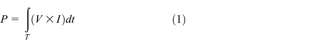
where ‘P’ is the power that flows through the electric circuit per unit of time, ‘V’ and ‘I’ are the PD voltage and PD current, respectively, and ‘T’ is the transient lapse time of each PD. The propagation direction of the power produced by a PD is given by sign of the equation 1 (Hayt, 2011).

The instantaneous power produced by a PD pulse that may flows in both directions for different times during the charge transient. However, the sign of the time integral of the instantaneous power indicates the propagation direction of the transient and is independent of the ‘V’ and ‘I’ waveforms.

Equation 1 implies the sign rule of algebraic multiplication: a change in sign in the voltage ‘V’ results in a change in sign of the current ‘I’ if the direction of the power flow remains constant.

The excitation voltage that produce the PD can be considered constant because its frequency is low in comparison to the transient associated with the PD that has a duration less of one microsecond (James et al., 2009). Therefore, the voltage can be taken out of the integral.

Finally, the integral of the current I(t) can be separated in two components, a positive part, I(+), and a negative part, I(-) of the PD waveform .

sgn [D] = sgn [V * (\int_{T} I (+) dt - \int_{T} I (-) dt)]

(2)

Equation 2 serves as the mathematical basis for the proposed measurement technique. The separation of the two current components I(+) and I(-) and their integration are carried out by signal processing and electronic circuits, which are described in detail in the following sections.

PD propagation

Power cables are designed to convey energy at low frequency, but their configuration makes PD pulses propagate as in a short transmission line.

Partial discharges in cables and accessories, such as joints and terminals, are produced by defects in the insulating material or, in general, in the interconnections between the associated accessories. A PD induces impulsive charge packets, which travel through the conductors that comprise the cables (James et al., 2009). The magnitudes of the PD parameters along the cable, such as the pulse amplitude and waveform, depend strongly on the propagation characteristics of the cable (El Mountassir et al., 2012).

Figure 1a shows a schematic representation of a PD traveling on a typical monophasic power cable, which behaves as a short transmission line. The cable shield is always grounded at least at one end for safety reasons, and only carries low frequency current when there is a fault or an imbalance in the power system. However, at high frequency, there are two main propagation modes: the differential mode (DM) and the common mode (CM). The termination impedances at the cable ends are Z1 and Z2 for the differential mode, and Z3 is the common mode impedance as depicted in Figure 1a.

Figure 1.

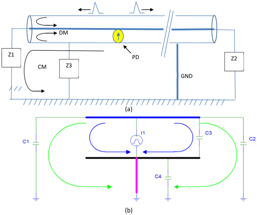
PD propagation modes in a power cable, including common mode and differential mode (a), and the simplified high frequency model (b).

In the DM propagation the currents, generated by the PD, flow through the central conductor until they arrive at the termination impedances and return through the cable shield. This configuration consists of a coaxial cable arrangement where, by symmetry, the magnetic fields produced by the PD are cancelled outside the cable; therefore, they are not detected by using external magnetic sensors.

In contrast, the high–frequency current of the CM propagation flows through the main conductor and return to the cable shield through the ground. The ground connections of the shield at the junctions or terminals are the paths through which the CM current flows. Hence, the current flowing through the main conductor and the cable shield are different and it can be measured by a magnetic field sensor. This current magnitude is a function of PD magnitude and all impedances associated with the cable and loads at high frequency. Consequently, the measured magnitude depends on each particular cable. The simplified transient model circuit is shown in Figure 1b.

Direction of propagation

Electric charges move owing to the presence of an electric potential. In the case of the transients produced by a PD within a cable, the charges move from higher to lower potentials based on the convention that the current moves from the positive to the negative terminal. Owing to the fact that the cable is a passive device, that is, it does not have internal energy sources if charge accumulation due to insulation is not considered; hence it only allows the movement of charges owing to the potential differences applied.

When the cable transports energy at the system frequency (50 or 60 Hz), the voltage changes periodically in a sinusoidal way and the sign alternates once every cycle. However, the current always flows from higher to lower potential. This also occurs with transient currents produced by PD. In contrast to the reactive power, which may flow in either direction, the real power flow always occurs from the source to the load. As an arbitrary convention, the real power is considered positive when it flows out of a component and negative when it flows into a component.

Figure 2 shows the waveforms of a PD current that propagates in a cable under a positive excitation voltage. Current I1 propagates from right to left, whereas current I2 propagates in the opposite direction. The change of direction corresponds to a change in the current’s sign; however, the two waveforms are equal and have opposite signs. If the current sensor polarity is inverted, the sign of the measured current will be also inverted.

Figure 2.

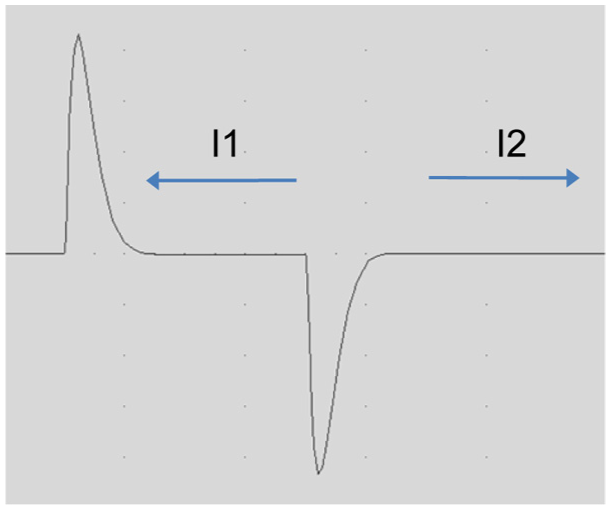
Charge injection generated by a PD that propagates in one direction (I1) and in the opposite direction (I2).

Measurement instrumentation

The instrumentation equipment consists of an electronic signal processing module connected to a sensor array that measures electromagnetic activity when it is placed on top of an active power cable. The currents generated by the PD are detected by means of an inductive magnetic detector, while a Hall Effect sensor provides a phase reference in order to plot the PD pattern.

Sensor array

Locating the sensors on the external surface of a high voltage cable, the PD electric signals are obtained through HFCT magnetic flux measurements at high frequencies, and low frequency sensor (LFS) by means of a Hall Effect sensor at low frequencies (50 to 60 Hz).

Phase reference sensor

When the cable is energized measurements of the potential are not available, therefore, the system obtains a phase reference (PHR) indirectly from the low–frequency magnetic flux produced by the current load in the cable. In the case of a unitary power factor (PF), the current and voltage phases are the same. If the PF is not unitary, a phase shift of

Δ RF = arc Cos (PF)

(3)

must be considered in order to plot the PD pattern, where PF is the operating power factor, and ΔFR is the phase shift that must be considered when the PD+D pattern is constructed.

The LFS sensor consists of a Hall Effect sensor with an array of flexible amorphous steel plates that guide and concentrate the magnetic flux. The signal from the LFS sensor is amplified and converted into a digital signal that is used as a phase reference, which gives a signal of logic ‘1’ when the sign of the current is positive and logic ‘0’ when it is negative. The sensitivity of the Hall Effect sensor is 2.5 mV/A; thus, a minimum of 3 A is required to correctly obtain the phase reference. The phase reference PHR from the LFS sensor is used to graph the PD+D pattern, representing the PD magnitude as a function of phase and coloured it according to propagation direction.

PD sensor

The PD electric signals are obtained via a HFCT sensor located over the high voltage cable external jacket for proper operation. The HFCT sensor operates in the band of 1 to 5 MHz. The sensitivity of the HFCT sensor, in the 1 MHz +- 5% band, is 5.0 mV/pC with a noise level of 20 mV; thus, its sensitivity is 4 pC.

The PD sensor consists of two coils serially connected and wound around two ferrite cores. These coils are mounted in a mechanical array that guarantees their alignment with the power cable to optimally detect the variations of the high–frequency magnetic flux. The mechanical support that holds the sensor array is flexible and adjusts to the cable diameter. This makes possible to obtain maximum sensitivity independently of the cable diameter. The sensor array has a polarity indicator with an arrow that is used as a reference direction. The shielding of the current sensor at high frequencies is indispensable to avoid detection of external electromagnetic noise that may interfere with the measurement of the propagation direction.

Signal processing

The electronic signal processing (SP) module takes as inputs the signals coming from the sensors array and yields as outputs a digital signal that represents the propagation direction of the PD as illustrated by a block diagram in Figure 3a and schematically in Figure 3b.

Figure 3.

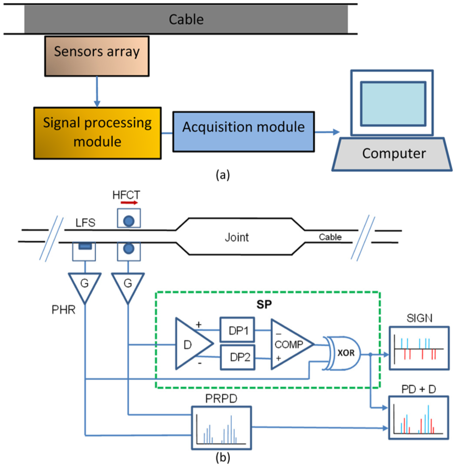
Instrumentation block diagram (a) and detail of the system used to obtain the PD+D pattern (b).

Figure 3b shows the inductive HFCT magnetic and LFS Hall effect sensors placed around the power cable. The signal processing module consists of a double–ended output differential amplifier (D), direct and inverted, of the inductive sensor. These signals are processed with their corresponding rectifiers and peak detectors DP1 and DP2. Subsequently, these signals are compared using a comparator (COMP) that produces the sign of the measured current. Finally, it is carried out a logic XOR of the COMP output and the PHR to obtain the vector SIGN, which assigns a colour to each PD in the PD+D pattern based on its direction.

Thus, a signal SIGN with a value of 1 indicates that the propagation direction coincides with the polarity of the sensor array, whereas a value of 0 indicates the opposite direction. The rectifiers and peak detectors DP1 and DP2 performs two functions: signal rectification and time integration of the PD. This process provides a time constant that widens the PD pulses so they can be correctly digitized at a considerably lower sampling speed than is required to do so directly from the inductive sensor’s output.

With the signal provided by the SP module, a SIGN vector is constructed for the detected PD for each cycle. If a PD is not detected simultaneously by both peak detectors (DP1 and DP2), the PD and its detected signal are discarded. Finally, the PD+D pattern is constructed by combining the well-known phase-resolved partial discharges (PRPD) and their directions. To carry out this task, a three–dimensional vector is formed with the magnitude, the colour associated with the direction, and the phase angle for each detected discharge. The PD+D pattern is updated at every cycle of the power signal by superimposing the new pulse on those obtained previously.

The following convention was established for plotting the PD+D pattern. PD that is plotted in grey colour propagates according with the direction indicated in the sensor array, whereas that in dark grey colour propagates in opposite direction to the polarity. The PD patterns are digitized, processed and displayed using 16 bits commercial acquisition cards with a sampling rate of 100 k samples/s, while a computer program that is implemented in a graphical language controls the data acquisition and display.

There are three main limitations to the equipment operation:

When the PD repetition frequency exceeds 20,000 discharges per second (20 KDP/s), the detection system operates incorrectly due to the integration time constant of the peak detectors, which favours the superposition of consecutive PD pulses. Hence, the signal acquisition sampling frequency limits the maximum repetition frequency.

When the discharge level is such that the amplifiers become saturated, the operational upper limit is exceeded, and the detection circuit operates incorrectly. This is corrected by incorporating an attenuation system that widens the dynamic range of operation.

There is a limit for the appropriate PD detection, which are determined by the minimum PD amplitude at which the signal–to–noise ratio in the measurement frequency band is 3 dB. This limit is defined as the lower limit.

The sensitivity of the detector depends on the gains of the input amplifiers which are variable. In the prototype system, the lower limit is 4 pC, and the upper limit is 20,000 pC.

Experimental setup

Figure 4 shows the experimental setup used to evaluate the proposed methodology. A 15-m-long 34 kV class, XLPE, wired screen cable section equipped with the corresponding terminals was connected to a high voltage power source.

Figure 4.

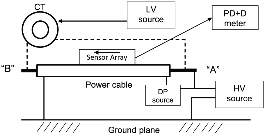
Experimental set up for verifying the sensor operation and detector direction.

A regulated high voltage power source from 0 to 100 kV, 3 mA (HV Source) was used to produce the PD and a 20 kV high voltage probe was used to voltage measurement. Overcurrent protections and insulating supports was also considered.

A current transformer (CT) fed by a regulated low voltage power source (LV Source) 30 A, variac transformer was used to produce a 10 Amp current through the cable main conductor. The current was verified to have the same voltage phase as the high voltage source, simulating the operation of a cable with a unitary power factor.

The sensor array was placed lengthwise in the middle of the cable as shown in Figure 5a, where an arrow is observed indicating the direction of polarity of the sensor array.

Figure 5.

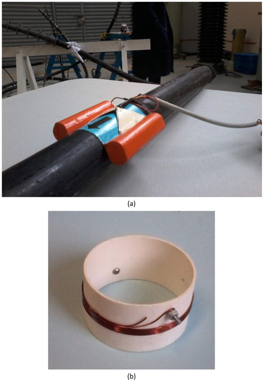
Sensor array used for PD detection on the test cable (a) and the barrier PD generator (b).

The experimental set up allows to simulate when PD occur at a point along a power cable buried in a trench using two cable segments and placing the PD source in their interconnection. In any case, the sensors array can only be placed on the cable at the manhole where the ends of the cable are available.

Results and discussion

A standard PD calibrator was placed between the main conductor’s ‘A’ end and the ground terminal as shown in Figure 4. This operation was performed without exciting the cable sample with a voltage and current. The sensitivity of the test circuit to an applied 200 pC pulse was 100 pC.

The change of direction detected by the instrument was verified by changing the polarity of the pulses generated by the calibrator and inverting the direction of the sensor array on the cable. The PD produced by the calibrator propagated through the main conductor and were capacitive coupled to ground, which allowed them to be detected by the sensor array. Under these measurement conditions, the common mode (CM) is favoured. The DM propagation mode occurs when the calibrator is connected to the ‘B’ end of the central conductor and ground, and the calibration pulses are not distinguished from the background noise. Following, an artificial controlled barrier type PD source, named Dielectric Barrier Discharge (DBD), was placed on end ‘A’ of the power cable (Figure 4), which initially configured the polarity of the sensor array in the direction toward end ‘B’.

The DBD source consisted of a capacitor formed by the geometric arrangement of two 22 AWG enamelled wires (each 1 m long) coiled side by side on a 750 mm diameter insulating cylinder as shown in Figure 5b. Then 1 kV and 10 Amp are applied to experimental setup.

The measured PD+D patterns are shown in Figures 6a and 6b. The PD activity measured throughout 100 cycles shows an average of 4770 discharges with a standard deviation of 112.

Figure 6.

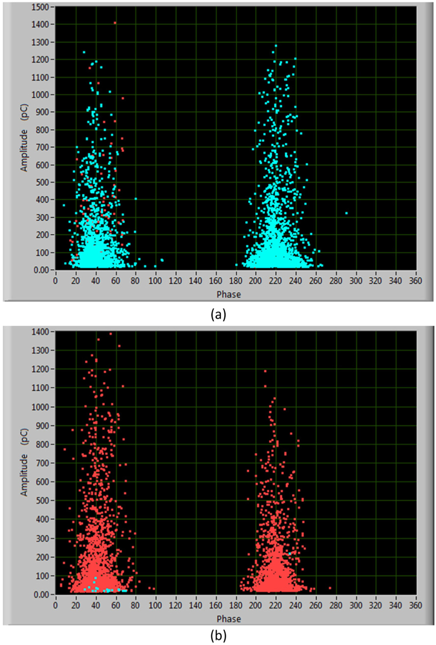
PD+D pattern obtained by the sensor array on top of the cable in a given direction (a) and rotated 180° (b).

Figure 6a shows the PD activity measured throughout 100 cycles. For the phase angles between 0° and 90° and between 180° and 270°, the blue plot indicates that the discharges propagate in the direction of the sensor array’s polarity; that is, the discharges propagate from ‘A’ to ‘B’.

The sensor array was then rotated 180° such that the direction of the sensor array’s polarity pointed toward end ‘A’, which produced the pattern shown in Figure 6b. The principal PD activity is in phase with that of Figure 6a, but the PDs are plotted in red. Therefore, the discharges propagate in the direction opposite to the polarity of the sensor array (from ‘A’ to ‘B’). Figures 6a and 6b show low activities in the opposite directions; that is, red discharges in Figure 6a and blue discharges in Figure 6b. These could be associated with reflections at the end of the cable.

Later, another test was conducted using 15 kV and 10 Amp, at the high voltage cable only without terminals.

Figure 7 shows PD measurements in which corona partial discharges can be observed over the background noise present at both ends of the cable energized at 15 kV in the absence of terminals connected at the ends.

Figure 7.

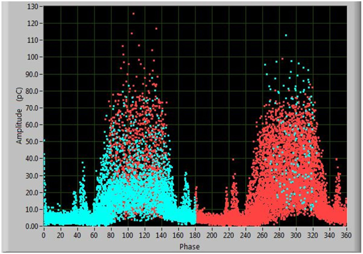
PD+D corona and noise pattern at both ends of the cable.

The maximum sensitivity is obtained by placing the sensor on the conductor grounding cable, however, any DP activity in a cable requires get out of service as soon as possible.

The technique has problems in identifying the propagation direction when the signal to noise ratio is lower than 3 dB. The detection errors were observed to be owing to the superposition of PDs that come from both directions. However, because the patterns are composed of many individual PD, the direction of the origin of the highest amplitude defect will be given by the dominant colour of the point cloud that forms the PD+D pattern.

Conclusions

This study presents a simple approach of PD source location in power cables that allows to know if the PD are propagating in the sensor polarity or in the opposite direction. Laboratory and field measurements were presented and demonstrate that the proposed technique for locating the propagation direction of the PD in a power cable operates correctly. It was also proved identification of PD activity and the location of its source in a power cable by means of magnetic sensors array. The proposed technique for detecting of PD propagation direction is based on the exclusive-or function over the waveforms polarity of PD and the phase reference.

Only a portion of the current produced by the PD is detected by the HFS, therefore, the measured quantities not represent the correct values of the DP. However, any PD activity detected in a cable should be revised. It is important to note that ‘cross bonding’ of the cable shields prevents the proposed method from functioning correctly because the phase references are interchanged. In this case, the measurement must be performed while temporarily reconfiguring the ground connections of the shields. This is a common practice for the use of any PD detection system in the field. Future work comprises optimizing of the electronic circuitry and the graphical interface to produce a complete set of diagnostic equipment. This device should be designed to operate while mounted on a pole to allow the user to take measurements at a longer distance from the manhole, which would improve safety conditions.

Footnotes

Declaration of conflicting interest

The authors declare that there is no conflict of interest.

Funding

This research received no specific grant from any funding agency in the public, commercial, or not-for-profit sectors.

References

Densley

(2001) Aging mechanisms and diagnostics for power cables, an overview. IEEE Electrical Insolation Magazine 17(1): 14–22.

El Mountassir

Stewart

McMeekin

Ahmadinia

(2012) Effect of noise on the location accuracy of partial discharges using radiated RF detection techniques. In: IEEE 47th International Universities Power Engineering Conference (UPEC), 4–7 September, Uxbridge, UK, pp. 1–6.

Gong

Sun

Zhao

(2014) Research on directional coupler measurement in partial discharge monitoring of XLPE cable. In: IEEE Proceedings of 2014 International Symposium on Electrical Insulating Materials (ISEIM), Niigata, Japan, 1–5 June, pp. 253–256.

Hayt

(2011) Engineering Electromagnetics (4th ed.). New York: McGraw-Hill.

Inatomi

Makki

Kozako

et al . (2014) Study of direction identification of partial discharge using multi small loop sensors. In: IEEE Proceedings of 2014 International Symposium on Electrical Insulating Materials (ISEIM), Niigata, Japan, 1–5 June, pp. 245–248.

Ishimaru

Kawada

(2011) Location of multiple partial discharge sources using MAP estimation for consecutive pulses. In: IEEE Proceedings of 2011 International Conference on Electrical Insulating Materials (ISEIM), Kyoto, Japan, 6–10 September, pp. 177–180.

James

Kulkarni

Parekh

(2009) Partial discharge in high voltage equipment-HV cable. In: IEEE 9th International Conference on Properties and Applications of Dielectric Materials, 2009. ICPADM 2009, Harbin, China, 19–23 July, pp. 445–448.

Kim

Youn

et al . (2014) High-resolution partial discharge location estimation in power cables. IEEE Transactions on Dielectrics and Electrical Insulation 21(2): 758–765.

Mardiana

(2011) Phase difference method for two-end partial discharge location in power cables. In: IEEE GCC Conference and Exhibition, Dubai, United Arab Emirates, 19–22 February, pp. 597–600.

10.

Mashikian

(2000) Partial discharge location as a diagnostic tool for power cables. In: IEEE Power Engineering Society Winter Meeting, Vol. 3, Singapore, 23–27 January, pp. 1604, 1608.

11.

Mashikian

Bansal

Northrop

(1990) Location and characterization of partial discharge sites in shielded power cables. IEEE Transactions on Power Delivery 5(2): 833–839.

12.

Polak

Sikorski

Siodla

(2014) Location of partial discharges sources using sensor arrays. In: 2014 International Conference on High Voltage Engineering and Application (ICHVE), Poznan, Poland, 8–11 September, pp. 1–4.

13.

Sack

(2010) A non-contact directional sensor for partial discharge measurements. In: Conference Record of the 2010 IEEE International Symposium on Electrical Insulation (ISEI), San Diego, California, 6–9 June, pp. 1–4.

14.

Shafiq

Lehtonen

Hussain

Kutt

(2014) Performance evaluation of PD monitoring technique integrated into medium voltage cable network for smart condition assessment. In: IEEE Electric Power Quality and Supply Reliability Conference, Rakvere, Estonia, 11–13 June, pp. 351–357.

15.

Shafiq

Kutt

Mahmood

et al . (2013a) An improved technique to determine the wave propagation velocity of medium voltage cables for PD diagnostics. In: IEEE 2013 12th International Conference on Environment and Electrical Engineering (EEEIC), Wroclaw, Poland, 5–8 May, pp. 539–544.

16.

Shafiq

Lehtonen

Isa

Kutt

(2013b) Online partial discharge diagnostics in medium voltage branched cable networks. In: IEEE 2013 4th International Conference on Power Engineering, Energy and Electrical Drives (POWERENG), Istanbul, Turkey, 13–17 May, pp. 246–251.

17.

Steiner

Reynolds

Weeks

(1992) Estimating the location of partial discharges in cables. IEEE Transactions on Electrical Insulation 27(1): 44–59.