
Abstract
Traditional fault diagnosis methods mainly depend on the vector model to describe a signal, which will lead to information loss and the curse of dimensionality. In order to overcome these problems, in this paper an improved multi-linear subspace (MLS) method and locally linear embedding (LLE) are integrated (MLSLLE) to extract significant features. To obtain more information, first it is suggested that multiple sensors should be used to sample the vibration signal of a machine from different positions; then, these data are projected into different subspaces, where each sample is represented as a tensor form, respectively; finally, higher-order singular value decomposition and LLE are introduced to extract significant features. Thus a fault diagnosis method is proposed based on MLSLLE and support vector machines. The advantages of the proposed fault diagnosis method are validated by two real bearing data sets.
Keywords
Introduction
In real-world applications, it is crucial for industrial production to monitor machines’ running states in real time (Li et al., 2016; Yin et al., 2015a). When a machine has faults, a fault diagnosis system can automatically notify the operators to correct the fault, reducing the harm to the industrial production. As we all know, because of a large amount of redundant information fault diagnosis has become far more challenging. Investigation of a highly efficient method to extract significant features from quantities of information has become an urgent issue.
Traditionally, most feature extraction methods focus on space transformation techniques (An and Tang, 2016; Du et al., 2016; Gao et al., 2016b; Yin et al., 2013), such as short-time Fourier transformation (Seryasat et al., 2012), wavelet transformation (WT) (Gaied, 2015), S transformation (ST) (Hao et al., 2016), and so on. The significant features are extracted in these transformed spaces, by which the class of a sample is recognized. However, these kinds of methods can only deal with simple data sets. In order to improve the capability to handle complex data sets, great effort has been made in manifold learning algorithms (Jialiang et al., 2016; Yin et al., 2012) which reduces the dimensionality by exploring the structure information of a data set. Manifold learning can be roughly divided into two categories: linear methods and nonlinear methods. Principal component analysis (PCA) (Zhou et al., 2014) is a classical linear algorithm. The advantage of PCA is that it can construct an explicit projection relationship between an original high-dimensional space and the corresponding embedding space, by which a new sample can be easily mapped into the low-dimensional space. Linear algorithms are not suitable for dealing with data sets whose distribution is nonlinear. Hence, some work has been done to improve the performance of linear algorithms Gao et al. (2016c). Gao constructs a physics model by the inductive thermography mechanism and utilizes sparse greedy-based PCA to deal with this model. Experimental tests have been conducted to verify the efficacy of the proposed method. Ding et al. (2016) propose locality sensitive batch feature extraction (LSBFE) by exploring both the local and the global discriminant structure of the data manifold, and a new gradient optimization model is proposed to obtain the final result. LSBFE has a strong capability to extract significant features of a data set, but LSBFE is a supervised method. When the labels of the data set are unknown, LSBFE will fail. Usually, a complex data set can be better treated by nonlinear manifold learning algorithms (Alkaya and Grimble, 2015; Ding et al., 2015; He, 2013; Wang and Yin, 2014; Yin et al., 2015b). Nonlinear methods explore local structures in the original space and compute the embedding result by these local structures. Locally linear embedding (LLE) (Cheng et al., 2016; Roweis and Saul, 2000) is an unsupervised nonlinear manifold learning algorithm. The computing speed of LLE is fast, and only two parameters need to be set, so LLE has been widely researched.
All the feature extraction methods mentioned above mainly depend on vector form. Vector form not only loses much significant information but also has the small sample size problem. Therefore, dimension reduction algorithms based on tensor form have greatly attracted some researchers within the past decade (Cichocki et al., 2015; Rong et al., 2012; Zhao and Wang, 2017). Tensor-based dimension reduction algorithms have been successfully applied in image processing (Vasilescu and Terzopoulos, 2003), target detection (Du and Zhang, 2014), and industrial process monitoring (Luo et al., 2014), among others (Liu et al., 2013). Many researchers have demonstrated that tensor-based dimension reduction algorithms can also be efficiently used in fault diagnosis (Liu et al., 2014). The multi-linear subspace (MLS) method is a type of classical dimension reduction method based on tensors (Luo et al., 2015; Zhang et al., 2015). As shown in Figure 1, the MLS method first describes a data set using tensor form; then, various decomposition technologies, such as Tucker (Louwerse and Smilde, 2000), higher-order singular value decomposition (HOSVD) (Afra and Gildin, 2016), multiple principal component analysis (MPCA) (Zhang et al., 2016) and parallel factor (PARAFAC) (Rasmus, 1997), are employed to project the data set to feature spaces. For instance, in order to obtain the most significant features, Nomikos and Macgregor (1995) allow MPCA to work directly on matrices (second-order tensors) and the experimental results illustrate that the performance of tensor-based methods is much better than that of vector-based methods. For inspecting a gear, Gao et al. (2016a) developed a physics-based multi-dimensional spatial transient stage tensor model to describe the thermo-optical flow pattern, and a canonical decomposition was introduced to deal with the tensor model. Tests of a helical gear with different cycles of contact fatigue are performed, and the result indicates that the proposed method is effective.
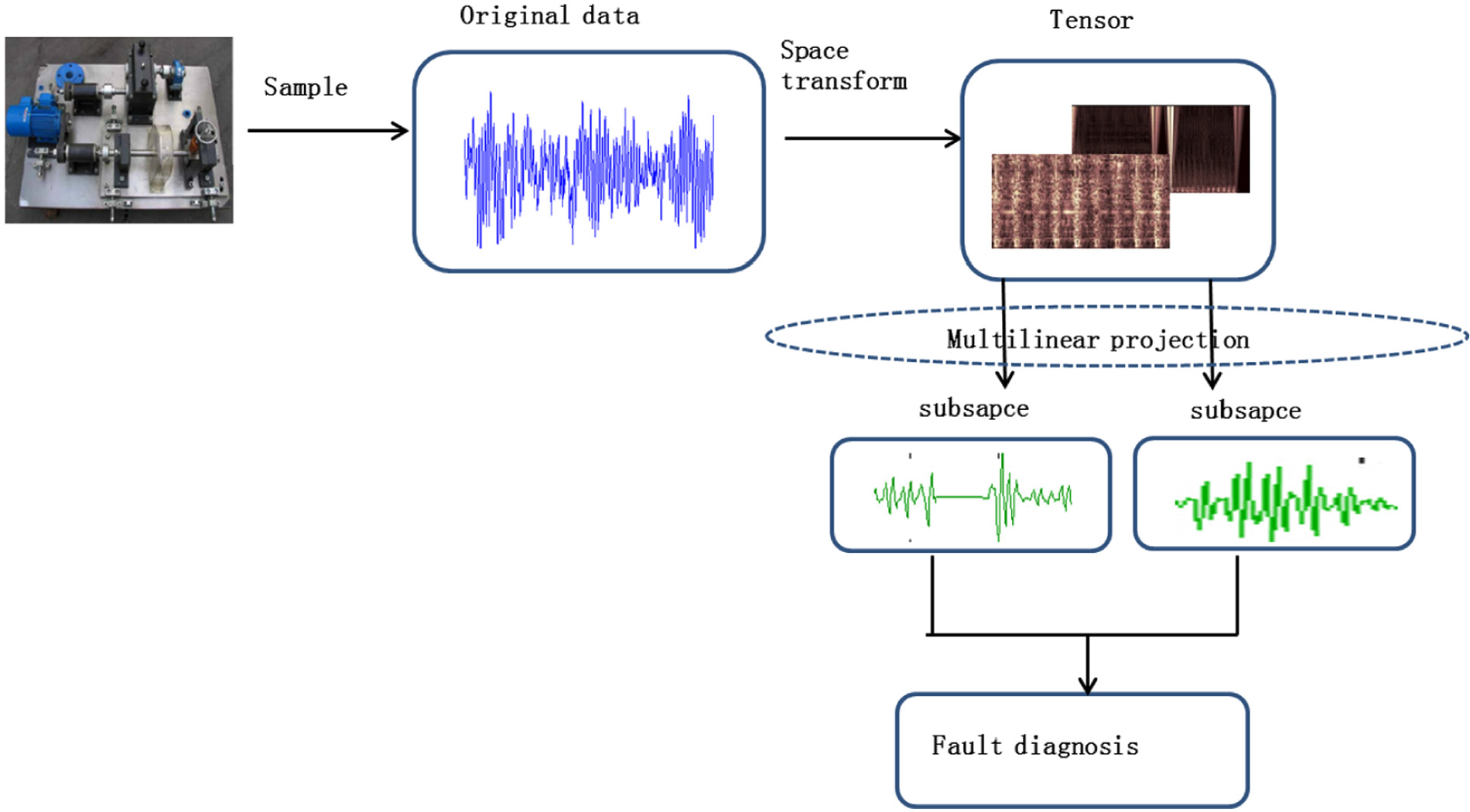
Multi-linear subspace process.
Usually, the expressions of a signal are different in various subspaces. If we can simultaneously observe this signal from all the subspaces, it will improve the recognition accuracy. MLS can project a signal into several subspaces. Most importantly, with all the factors considered in each subspace, we can better observe the signal. Hence, in this paper, we propose a new feature extraction method called MLSLLE that constructs a tensor for each sample and decomposes these tensors by HOSVD respectively, based on which LLE is employed to obtain the final features. The rest of this paper is organized as follows: in ‘Feature extraction’, the process of MLSLLE is illustrated in detail. Based on MLSLLE, a highly efficient fault diagnosis method is presented in ‘Fault diagnosis’. Experiments on two real bearing data sets are reported in ‘Experiments’. Finally, the conclusion is given in the last section.
Feature extraction
Basically, a tensor is just a high-order matrix that can utilize most known information in a frame to describe a signal. It is beneficial for us to fully observe a signal using a tensor model. This is illustrated by Figure 2. In this paper, we will perform WT and ST on the data sampled from different sensors and construct a tensor for each sample.
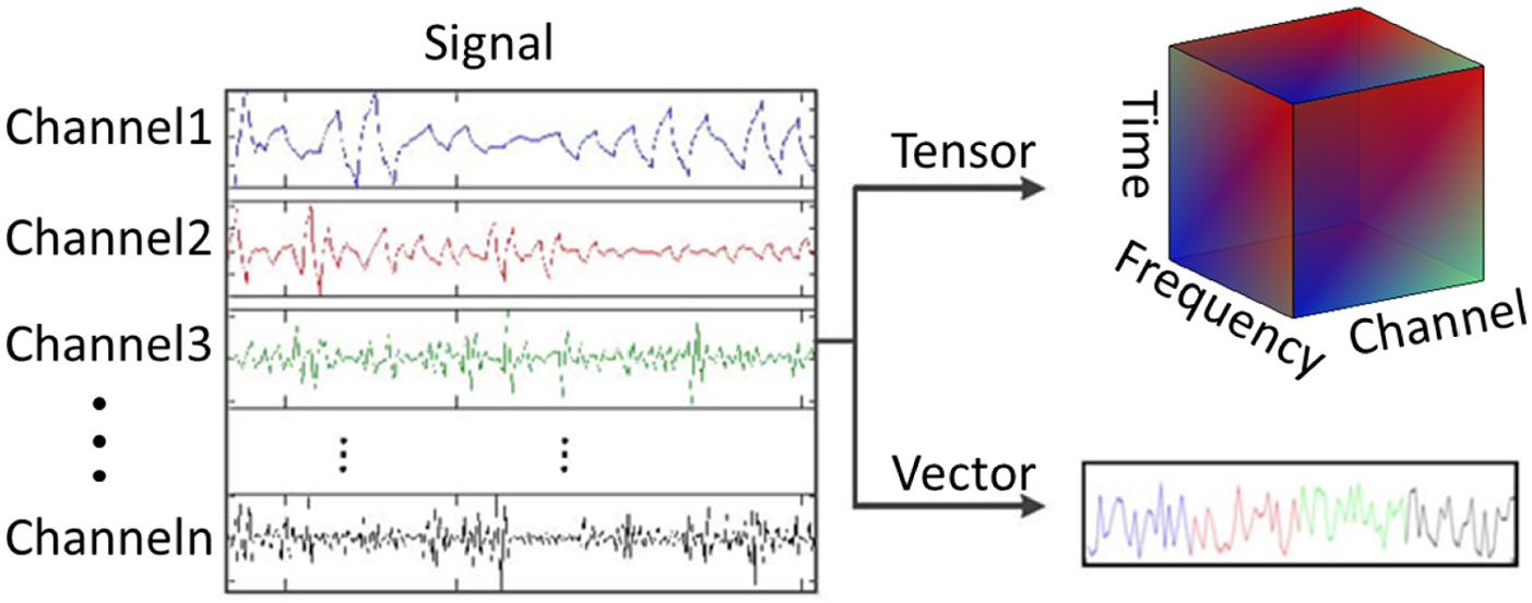
Comparing tensor form with vector form.
WT
WT is one of the classical signal processing tools, and is frequently used in analysing non-stationary signals. WT can project a signal into time–frequency space, where some significant features can be easily found. Let
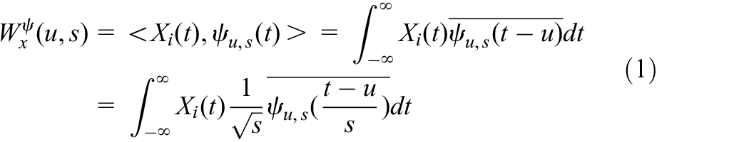
where
where
We project each sample to a time–frequency space by WT, and the
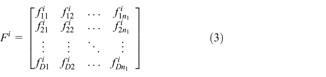
where
ST
ST is an extension of WT and it can overcome some disadvantages of WT. Unlike WT, ST can simultaneously provide the amplitude and the phase information, and, furthermore, ST is not sensitive to noise. ST can be defined as (Lin and Meng, 2011)

where
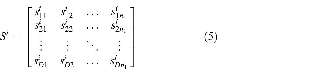
where
Tensor construction and decomposition
In this case, based on the two time–frequency spaces built above, we construct a tensor model for each sample. The number of subspaces is two, and the size of each subspace is
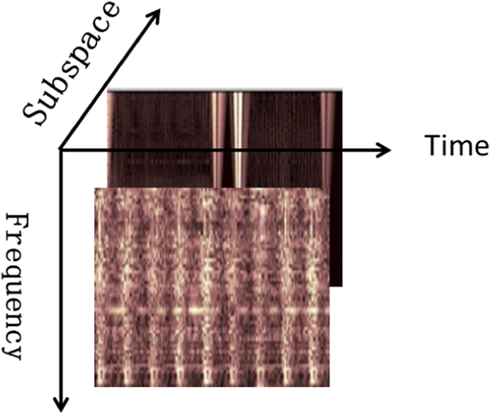
Tensor representation.
In order to explore the intrinsic features of a tensor, HOSVD, that is, an extension of singular value decomposition (SVD), is employed to decompose the tensor. Compared with SVD, HOSVD is more efficient at extracting significant features. Before decomposition, HOSVD must flatten a tensor to a series of matrices along various dimensions of the tensor (see Figure 4). Then SVD is introduced to decompose these matrices, that is, HOSVD still works based on the matrix. However, the matrix flattened by the tensor contains all the information regarding various factors. For example,
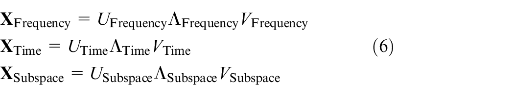
where
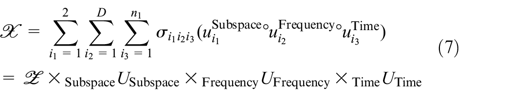
where ∘ denotes the outer product,

where

where the
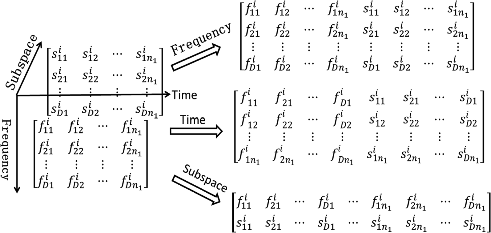
Flattening a tensor along different dimensions.
LLE
Although
Compute the neighbours of each point by the k nearest neighbor (k-NN) method or
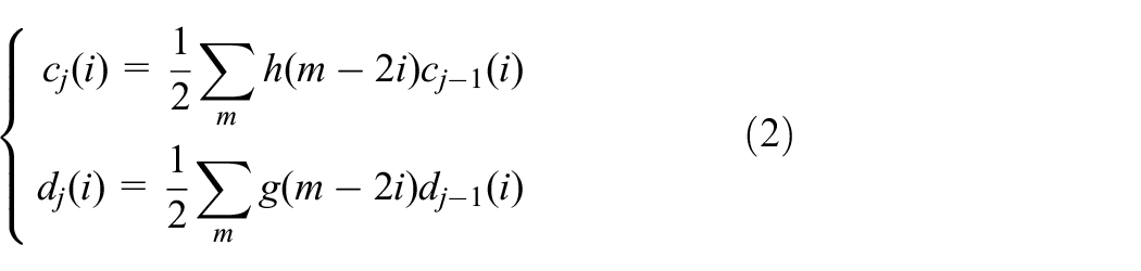
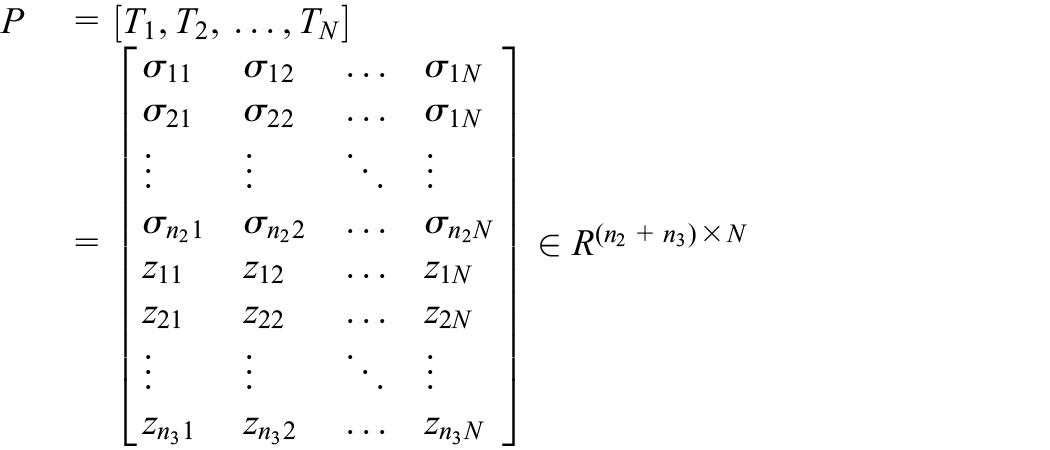
Explore the local structure information from the original data set. LLE treats the local reconstruction weight coefficient as the structure information. The weight coefficients can be computed as follows:
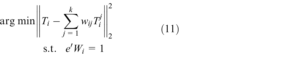
where

Compute the embedding result
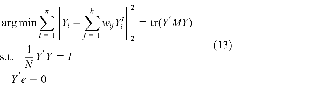
where
Fault diagnosis
Based on the MLSLLE algorithm, a novel machinery fault diagnosis method is developed. First, the features of the training and test data sets are simultaneously extracted by MLSLLE; then, the support vector machine (SVM) is trained by the features of training data set; finally, the classes of the test samples are recognized by the trained SVM. The complete fault diagnosis process is shown in Figure 5, and the detailed description of the process is as follows.
Sample the data from a machine, then divide the data into training and test samples.
WT and ST are introduced to decompose each sample respectively, by which a tensor form of each sample is constructed.
Respectively perform HOSVD on the constructed tensors to obtain the initial features
Reduce the dimensionality of
Train SVM in the low-dimensional space obtained by step 4.
Compute the features of the test samples by the technology described in step 2 to step 4.
Recognize the classes of the test samples using the trained SVM.
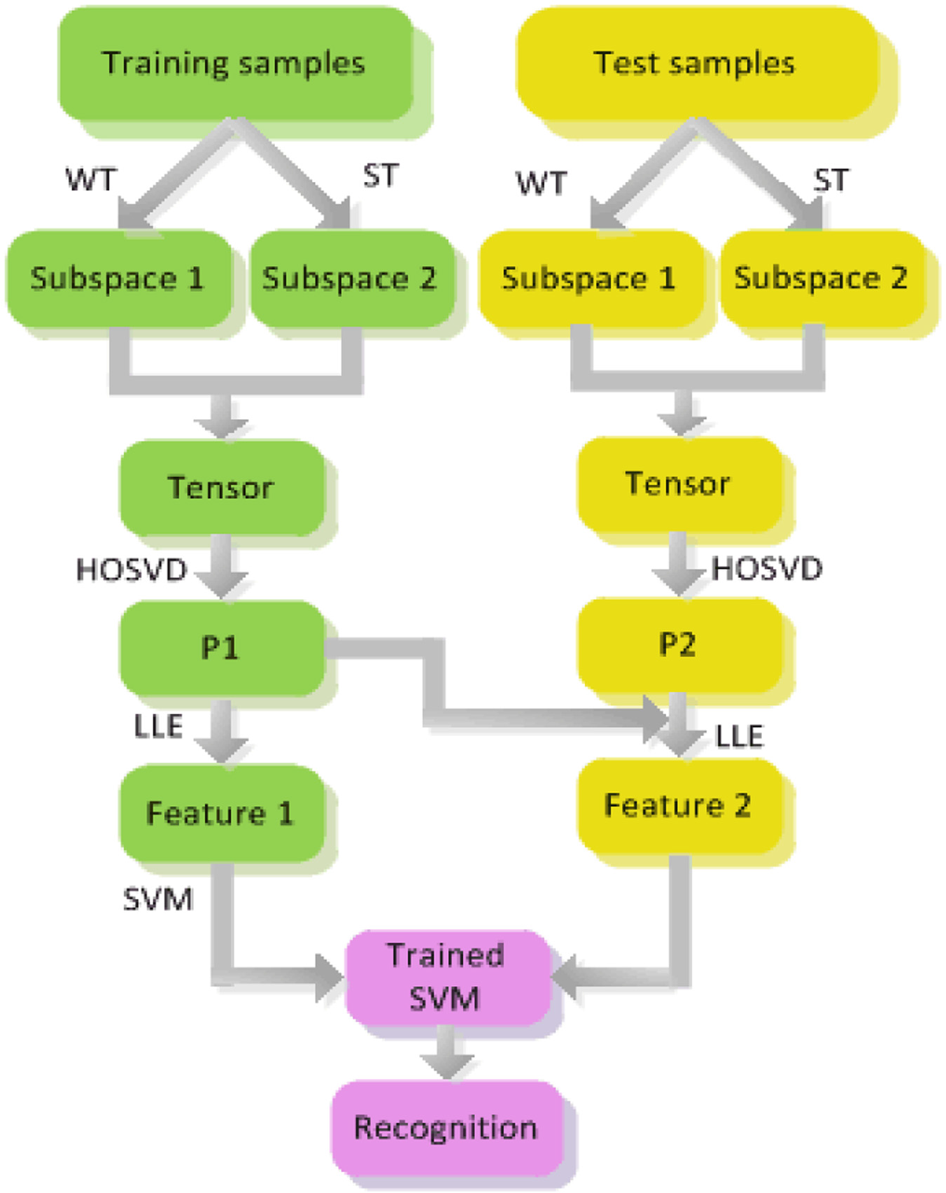
Fault diagnosis based on MLSLLE.
Experiments
In this section, two real bearing data sets are utilized to validate the effectiveness of our proposed method.
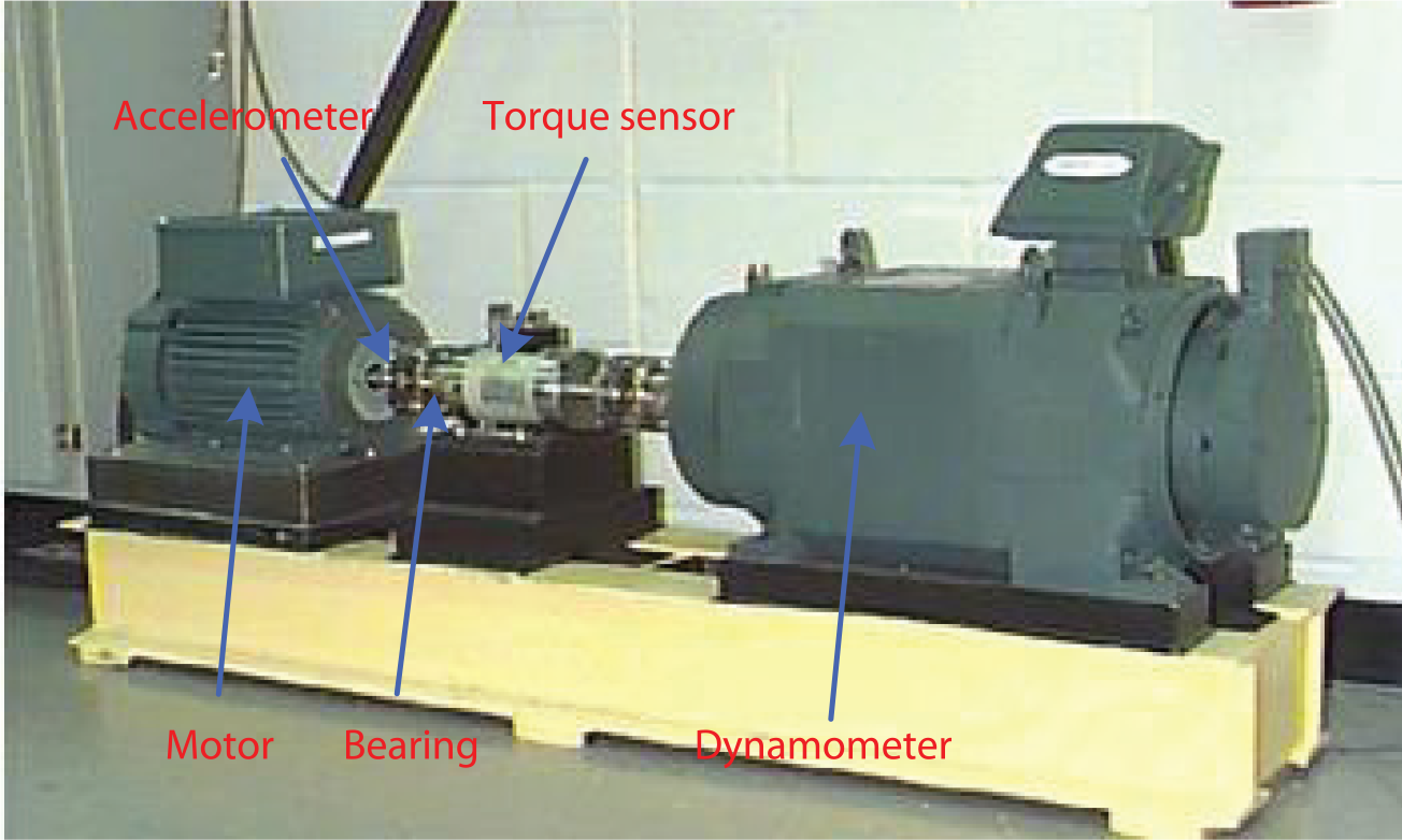
Bearing test platform 1.
Time-domain signals of bearing data set 1.
In this experiment, we mainly analyse the performance of MLSLLE in terms of feature extraction. According to the characters of the signal, sym3 is selected as the mother wavelet, and each sample is decomposed into eight layers by WT. In addition, to ensure that the sizes of the two subspaces are equal, we only select eight important frequency ranges from ST. In order to compare their capability for feature extraction, PCA, tensor locality preserving projections (TENSORLPP) (He et al., 2005, 2006), conventional MLS and our improved MLS are all performed on the bearing data set, and the most significant feature and the top three significant features of each sample are shown in Figure 8.
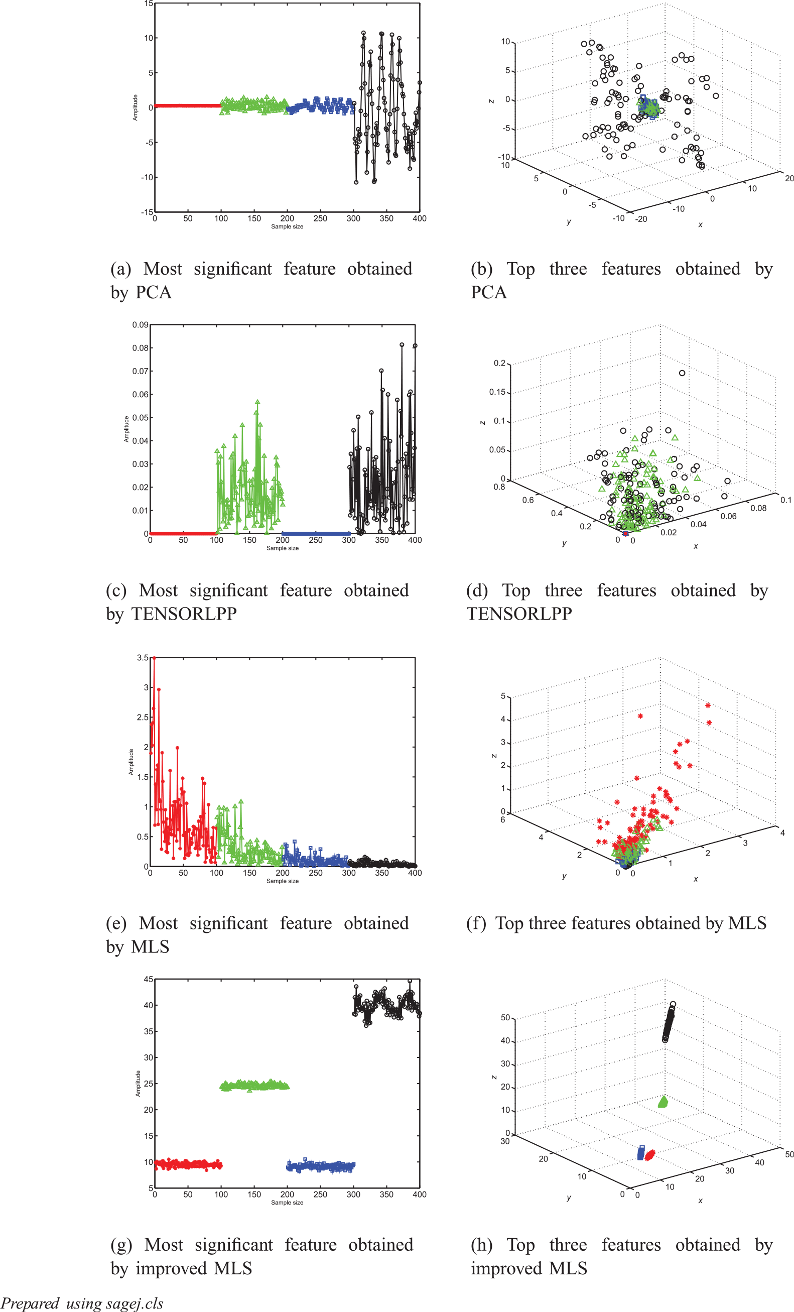
Features of bearing data 1 extracted by different algorithms. (The red ‘*’ denotes ball fault data; the green ‘▵’ represents inner race fault data; the blue ‘□’ denotes outer race fault data; the black ‘o’ indicates normal data.)
Since PCA belongs to a linear dimension reduction algorithm, PCA can only deal with simple linear data sets. Hence, the features extracted by PCA are not suitable for classification. The fact can be demonstrated by Figure 8(a) and 8(b), where most of the samples overlap. Although TENSORLPP and MLS describe a signal using tensor models, all the algorithms construct a tensor model for the whole data set, for which features of each sample are only extracted from the tensor model. In other words, TENSORLPP and MLS belong to global algorithms ignoring the local information, so the features obtained by the two algorithms are still not suitable for recognition. As shown in Figure 8(g) and 8(h), although the two kinds of data are close, all the samples can be recognized in three-dimensional space. This is because each sample is described in tensor form, increasing the amount of useful information. Furthermore, the features of each sample are independently extracted, which will be benefit feature extraction. We perform the K-NN method on the one-dimensional and the three-dimensional feature spaces obtained by improved MLS, and find that the normal and the inner samples can be fully recognized (accuracy can reach 100%). Because the features of the ball and outer samples are very similar in one-dimensional space, K-NN method cannot distinguish between the two classes. However, in three-dimensional space, the inter-class separability between the ball and outer samples increases, so the recognition accuracy is 100%. Finally, we use LLE to reduce the dimensions of the features obtained by improved MLS (
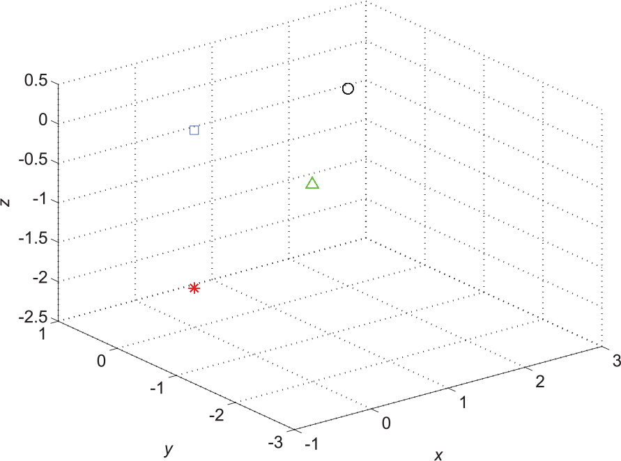
Features of bearing data set 1 extracted by MLSLLE. (The red ‘*’ denotes ball fault data; the green ‘▵’ represents inner race fault data; the blue ‘□’ denotes outer race fault data; the black ‘o’ indicates normal data.)
The computational cost of MLSLLE can be roughly divided into three parts including tensor construction, HOSVD decomposition and LLE. In order to test the computational cost of MLSLLE, we use MLSLLE to deal with the bearing data set, whose size is 400 and whose dimensionality is 1024. The result shows that MLSLLE only takes 15.6 s to deal with this data set, so MLSLLE can meet the requirements of industrial applications.
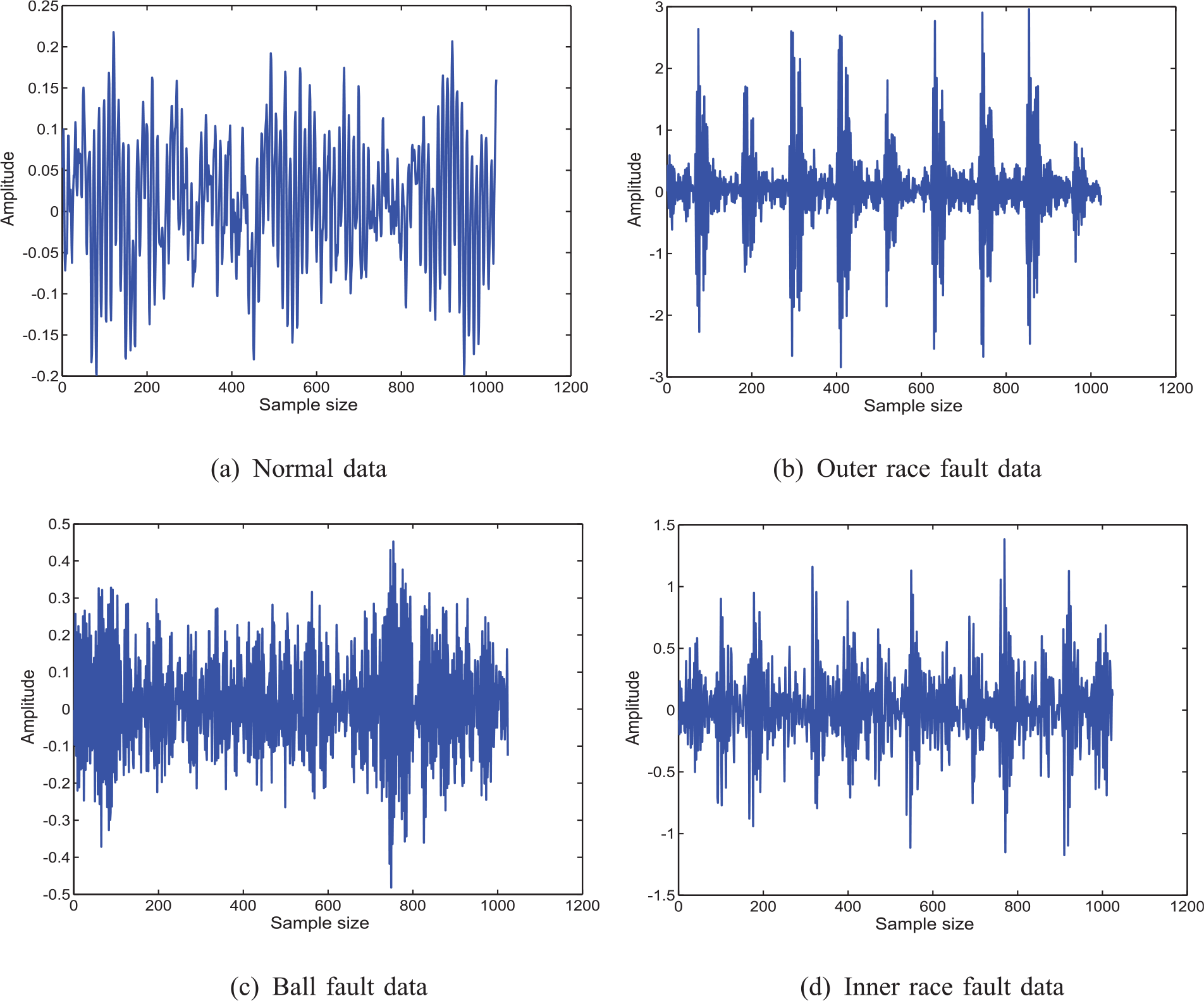
Bearing data set 2: This bearing data set is collected from a real test platform installed in our own laboratory. As shown in Figure 10(a), the test platform mainly consists of a motor, a gearbox and a bearing. Each kind of data can be generated by replacing bearings with different faults (see Figure 10(b)). It can generate four kinds of data: normal data, inner race fault data, outer race fault data and ball fault data. All the data is sampled from two accelerometer sensors mounted in the test platform’s horizontal and vertical directions. The bearing is driven by the rotating motor with a frequency of 1200 rpm, and the sampling frequency is set to 10 kHz. For convenience, the feature number of each sample is 1024, and the size of each type of data is 80. The one-dimensional signals in the time domain are shown in Figure 11.
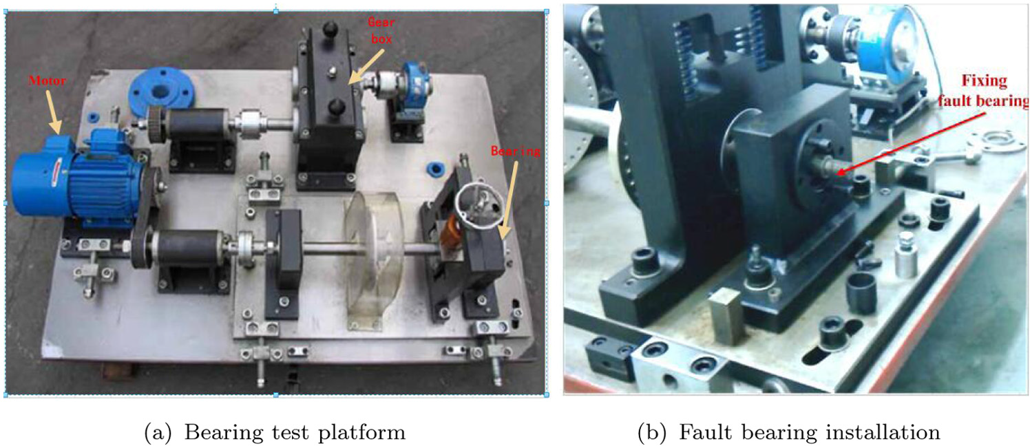
Bearing test platform 2.
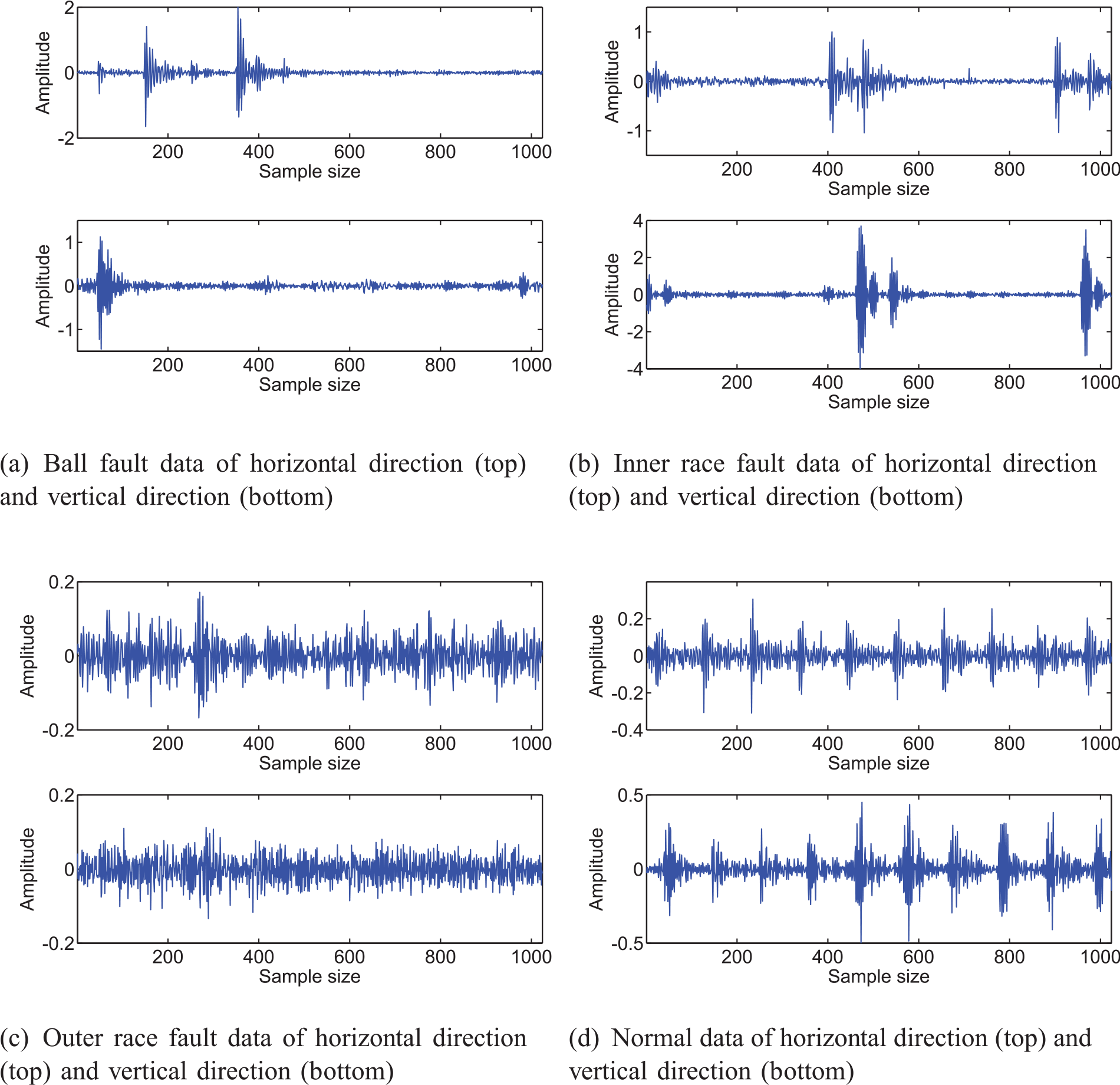
Four typical vibration signals of bearing data set 2.
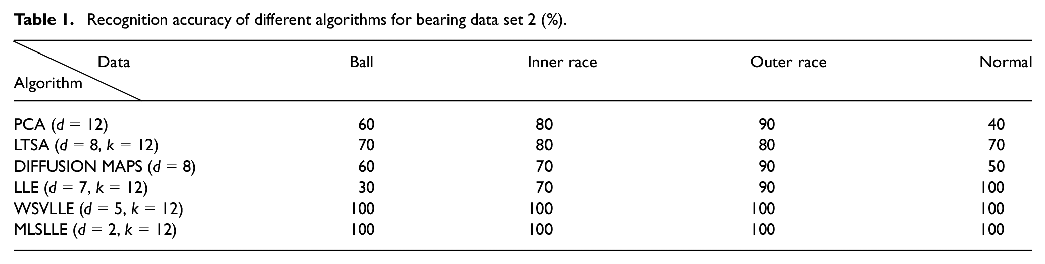
In this experiment, we addressed a classification problem using bearing data set 2. MLSLLE is used on the data sets to extract the features. Additionally, PCA, local tangent space alignment (LTSA), WSVLLE (Liu et al., 2016), DIFFUSION MAP, and LLE are also introduced to deal with the data set sampled from the vertical direction, for comparison with MLSLLE. All the optimal parameters of these algorithms are selected, and the visualizations are shown in Figure 12. It is clear that the features extracted by the algorithms depending on vector models completely overlap in three-dimensional space, and the classes of each sample cannot be directly recognized. Since they use tensor models, the features obtained by WSVLLE and MLSLLE have better intra-class compactness and inter-class separability. Finally, we conduct SVM on the embedding results to quantitatively analyse the performance of our proposed method in machinery fault diagnosis. The highest accuracy of each algorithm and the corresponding dimensionality are listed in Table 1. Although the accuracy of both WSVLLE and MLSLLE is 100%, the minimum dimensionality of features obtained by WSVLLE and MLSLLE is five and two, respectively. It implies that the features obtained by MLSLLE are more significant than the ones obtained by WSVLLE, so our proposed method has perfect performance in terms of fault diagnosis.
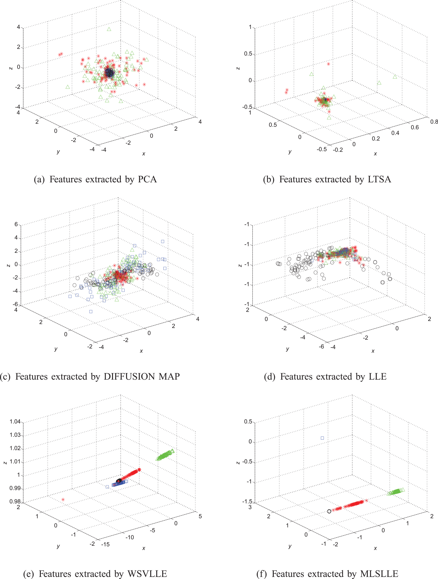
Features of bearing data 2 extracted by different algorithms. (The red ‘*’ denotes ball fault data; the green ‘▵’ represents inner race fault data; the blue ‘□’ denotes outer race fault data; the black ‘o’ indicates normal data.)
Recognition accuracy of different algorithms for bearing data set 2 (%).
Conclusion
This paper developed a tensor-based machinery fault diagnosis method called MLSLLE. MLSLLE uses the tensor model to describe each sample and employs HOSVD and LLE to explore the intrinsic features. We performed the proposed fault diagnosis method on two real bearing data sets, and the experimental results show that the proposed method can efficiently extract significant features and can obtain high recognition accuracy. In future work we will mainly consider how to directly use the tensor form with LLE. We will also take note of supervised or semi-supervised MLSLLE cases.
Footnotes
Declaration of conflicting interests
The authors declare that there is no conflict of interest.
Funding
This work is supported by the National Natural Science Foundation of China (number 61673102).