Hybrid extended-unscented Kalman filters (HEUKFs) for continuous-time nonlinear fractional-order systems with process and measurement noises are investigated in this paper. The Grünwald-Letnikov difference and the fractional-order average derivative (FOAD) method are adopted to discretize the investigated nonlinear fractional-order system, and the nonlinear functions in the system description are coped with the extended Kalman filter (EKF) and the unscented Kalman filter (UKF). The first-order Taylor expansion used in the EKF method is performed for the nonlinear function at the current time. Meanwhile, the unscented transformation used in the UKF is also concerned for the nonlinear function at the previous time. By using the HEUKF designed in this paper, the third-order approximations for the nonlinear function can be achieved to enhance the accuracy of state estimation and estimation error matrix. Finally, numerical examples are provided to illustrate the effectiveness of the proposed HEUKF for nonlinear fractional-order systems.
The thought of fractional-order calculus originates from an extension of integral-order calculus, and this idea can be traced back to 1695 by Leibniz and Hopital. For recent years, many engineers have been interested in this powerful tool, and the fractional-order calculus has been developed into an independent academic subject in Machado et al. (2014). The fractional-order calculus has been found to be a very useful tool to simulate the behaviors of real-world systems in Huang et al. (2018). Also, fractional-order models are more accurate than traditional models to reveal the dynamic of complex systems. Therefore, fractional-order models have been widely applied in the economics in Tarasov and Tarasova (2018), the biotechnology in Ionescu et al. (2017), the energy engineering in Huang et al. (2018), the agricultural engineering in Zhang et al. (2013), the automation and control in Sadeghzadeh and Momeni (2016) and so on. Besides, the fractional-order calculus has developed rapidly in the field of control engineering to produce many fractional-order controllers, such as the fractional-order sliding mode controller in Zhan and Liu (2018), the fractional-order proportional-integral- derivative (PID) controller in Hamamci (2008), the fractional-order fuzzy control in Li et al. (2018) and so on.
The memory property of fractional-order calculus can be used to reveal the essential properties and behaviors of real-world systems in Tarasov and Tarasova, (2018) and Pu et al., (2018). In the field of science and engineering, fractional-order calculus has been considered as an ideal mathematical tool to characterize complex systems with memory properties. For a fractional-order control system, the analysis of system stability and performance are of great significance to guide the design of fractional-order controllers. Because some controllers need to obtain the state information, it is very essential to estimate the state information effectively. Noting that the sampling values of measurement signals in fractional-order control systems are often subjected to many types of noises, some filters are required to gain the effective state information. Besides, some state information can not be measured directly, we also need to adopt some filters to obtain the state estimations such as the filter in Chen et al. (2018), the particle filter in Dong et al. (2018) and so on.
Kalman filter (KF) is an optimized algorithm to estimate the state information in the presence of noises, and it is increasingly widely used in real-world systems. In Sierociuk and Ziubinski, (2014), the estimation scheme of integer-order state space system was proposed, which is also suitable for nonlinear systems. In Simon (2010), various methods of incorporating state constraints into KF and its nonlinear correction was presented. A closed-loop adaptive KF for nonlinear continuous-time and discrete-time systems was presented in Wang et al. (2018). In Zhang JF et al. (2017), the robust optimal filter issue for one type of linear time-invariant systems with stochastic uncertainties was studied. For the problem that stochastic faults and unknown inputs seriously affect the performance of KF in engineering, the adaptive three-stage extended Kalman filter (EKF) for nonlinear systems was proposed in Xiao et al., (2018). In He et al., (2013), the parameters of the model were self-tuned based on unscented Kalman filter (UKF) and the state estimation was carried out under charge experiments. Moreover, the cubature Kalman filter (CKF) was also an effective state estimation method for nonlinear control systems. A variational Bayesian adaptive CKF was proposed for nonlinear state estimation in Miao et al. (2017). In Zhang L et al. (2017), a robust measure of nonlinear CKF was proposed to reduce the computational complexity and obtain satisfactory performance.
KF is generally used for integer-order systems, but the study of KF for fractional-order systems has been reported recently. In the wake of the development of fractional-order applications, fractional-order Kalman filters (FKFs) have been widely investigated in Yang et al. (2019). In Gao (2018), the FKF based on Tustin generating function for continuous-time fractional-order systems was demonstrated. FKFs can deal with correlated and uncorrelated process and measurement noises in Liu et al. (2019) in continuous-time fractional-order systems. The FKF can more accurately solve the state estimation issues for fractional-order systems in Chen and Zhanmei (2012) and Sierociuk and Dzielinski (2006). A KF was investigated based on some conditions of solvability, regularity and causality for discrete-time linear stochastic fractional-order singular systems in Nosrati and Shafiee (2018). In Zarei and Tabatabaei (2018), FKF for estimating the state information of discrete-time linear fractional-order systems with unknown disturbances was investigated. The KF algorithm in the discrete-time linear and nonlinear fractional-order systems was discussed in Sadeghian et al. (2013) and Nosrati and Shafiee (2018). A method of designing a fuzzy FKF was proposed to estimate the states with noises in Senthil et al. (2006). Furthermore, the non-Gaussian noise problem is an important issue in the design of fractional-order Kalman filters such as Lévy noises, colored noises and Brownian noises in Zhou et al. (2017). In Sun et al. (2017), the design strategies on fractional-order EKFs for discrete-time fractional-order nonlinear systems involving Lévy noises were proposed. The EKF algorithm for state estimations of nonlinear fractional-order systems with colored measurement noises in Safarinejadian et al. (2018) was proposed. For some systems with strong nonlinearity, the estimation effect of the EKF algorithm is not satisfactory. Hence, the UKF was considered to improve the estimation accuracy of fractional-order systems in Gao et al. (2019). A method based on fuzzy logic was proposed to improve the fractional-order UKF with the adaptive noise covariance in Ramezani and Safarinejadian (2018), and the convergence and accuracy of the state estimation was improved. The application of UKF in non-Gaussian measurement noises for nonlinear systems was studied in Zhu et al. (2018). Meanwhile, fractional-order UKF was investigated to estimate the state of charge, and the static and dynamic discharge experiments of the battery in Sun et al. (2011).
The accuracy of state estimation for nonlinear fractional-order systems based on nonlinear Kalman filters is determined by the treating on nonlinear functions in the system models. In this paper, the fractional-order average derivative (FOAD) method discussed in Yang et al. (2018) is used to discretize the investigated nonlinear fractional-order system, and the corresponding difference equation is established to improve the estimate accuracy. In the discretized system model, there are nonlinear functions related to the current time and the previous time. The first-order Taylor expansion and unscented transformation are used to deal with the nonlinear functions respectively. This paper combines the advantages of two treating methods for nonlinear function to improve the accuracy of state estimation to propose the hybrid extended-unscented Kalman filters (HEUKFs) for nonlinear fractional-order systems.
The main highlights of this paper are summarized as follows: (1) The estimation of nonlinear continuous-time fractional-order system is discretized by fractional-order average derivative in Yang et al. (2018) and the Grünwald-Letnikov differential (GLD) definition in Gao et al. (2019), and the sampling period is also a parameter of the nonlinear function. The nonlinear difference equation is obtained to reveal the dynamic characteristics. (2) The design of HEUKF based on FOAD method is further studied, and the theoretical basis of the third-order approximations of nonlinear functions in the system is given. Theoretically, the fractional-order HEUKFs are better state estimation compared with the fractional-order EKF and UKF based on GLD definition. (3) Compared with the UKF based on GLD definition, the HEUKF proposed in this paper can effectively estimate the state changed dramatically in a sampling period. (4) For fractional-order systems involving process and measurement noises, this paper proposes HEUKF to deal with uncorrelated noise problems. (5) Considering the computational burden in engineering applications, the HEUKF algorithm proposed in this paper is discussed to achieve effectively truncation.
The remaining sections of this paper are summarized as follows. In Section 2, we firstly use the definition of fractional-order calculus, and the discretized nonlinear fractional-order systems using FOAD are proposed. In Section 3, the design method of HEUKF is discussed, and the accuracy of estimation is also analyzed. In Section 4, two simulation examples are presented to test and verify the effectiveness of the investigated fractional-order HEUKF algorithm. Finally, the conclusion is given in Section 5.
By using the Caputo definition, we consider an estimated nonlinear system containing process and measurement noises to be investigated as follows
where is the -order derivative with . The state vector, the input and the measurement output are represented as , and respectively, the nonlinear functions are represented by and with class, and and are the process and measurement noises respectively.
For the convenience of calculation, the sampling period is denoted as the sampling time . , and are defined as the sampling values of , and . The mathematical expectations of and are , and is the zero matrix or vector with the appropriate dimension. Meanwhile, the covariance matrices of and are and , and and are uncorrelated.
By using the GLD definition, the derivative can be approximated by
where
In order to gain more accurate estimation, we further investigate design KFs based on FOAD method for nonlinear systems with the uncorrelated noises. Within a sampling period , the derivative can be approximated using the FOAD method for as
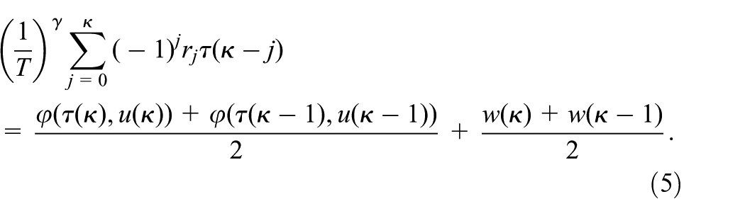
Therefore, the fractional-order nonlinear system (1) can be descretized by (4) as follows
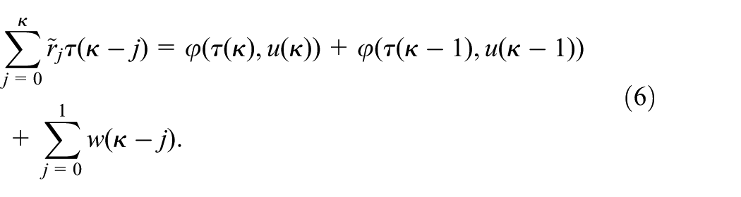
By choosing , the equation (5) can be represented by
Compared with the UKF and EKF based on the GLD definition, the FOAD method can further strengthen the accuracy of state estimation. In the following section, HEUKFs for nonlinear fractional-order systems are proposed.
Main results
Design method of hybrid extended-unscented Kalman filters
In this subsection, the design method of the corresponding HEUKF is studied with the uncorrelated noises on the difference equation (6) derived by the GLD definition. According to the design method of extended Kalman filter, the calculation method of the first-order Taylor expansion is given for the nonlinear function at the current time.
The estimation of is defined as , where involves , then the first-order Taylor expression of the nonlinear function at is given as follows
where
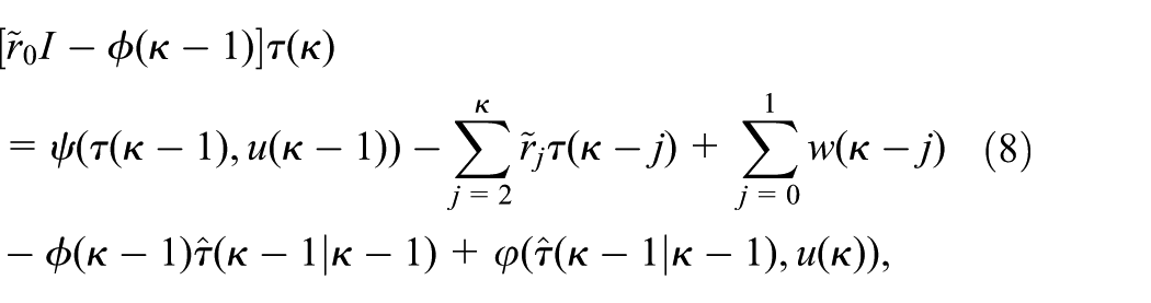
Defining the nonlinear function and substituting (7) into (6), we have
where is the identity matrix.
The nonlinear function and the matrices , are denoted for as follows
Meanwhile, and are determined by and , which are used in the proposed HEUKFs.
Therefore, the difference equation (6) can be represented by
Then, the predication of is defined as , where relates to , , …, , , ,…,. We assume that the condition can be obtained as follows
For the uncorrelated noises and , the unscented Kalman filter is investigated. According to the viewpoint of unscented transformation (U-T), the calculation method of the points in terms of the nonlinear function is given as below
where , is the square root of the matrix , is the th row of the matrix , , is a very small positive number, for white Gaussian noises and is the estimation error matrix for th iteration.
We investigate the estimation of and with for . By defining symbol , the Taylor expansion for the nonlinear function with respect to at is given by
By denoting , we obtain
For the function term , we get
We assume that is a mathematical expectation of the random variable . If the probability density is symmetric with respect to , we have for .
From (14), the estimation of the nonlinear function with the definition of as can be represented by
where .
From the points defined by (11), the nonlinear function is yielded by . According to for and for , the Taylor expansion of at for is determined by
where
For the case , we know that holds to obtain
We denote the following weights to estimate using points as
Accordingly, we get
Because the variable is symmetric with respect to mathematical expectation , we get for , it follows that
By using the condition (22), equation (21) can be rewritten as follows
where .
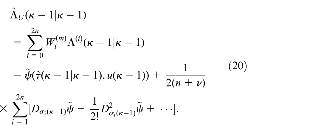
From (15) and (23), the th order terms with in and are similar to achieve the third-order approximations. If is used to replace , a more satisfactory approximation of in (10) is achieved.
Substituting (15) into (10), we obtain
Replacing with into (10), we also obtain
Consequently, the three-order approximations with respect to can be achieved by replacing with .
Approximations of state predication and predication error matrix
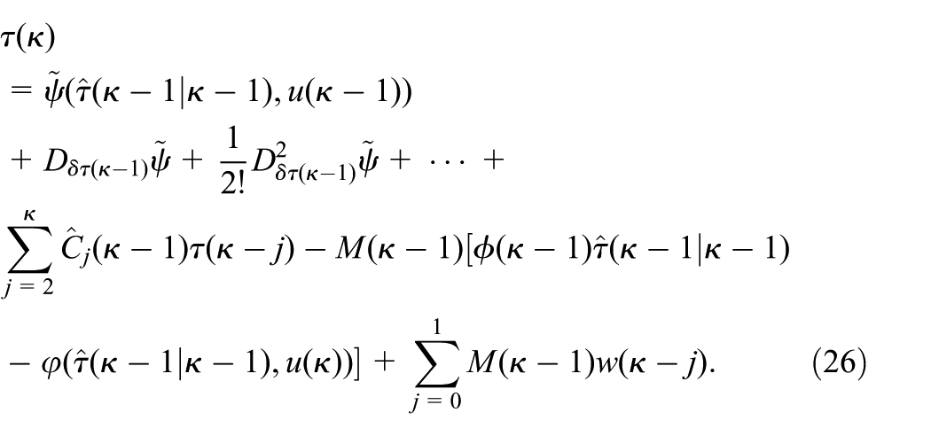
Substituting (13) into (9), the difference equation (9) can be represented by
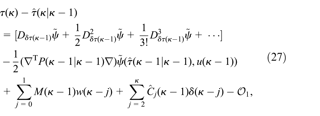
From (24) and (26), the predication error is calculated as follows
where .
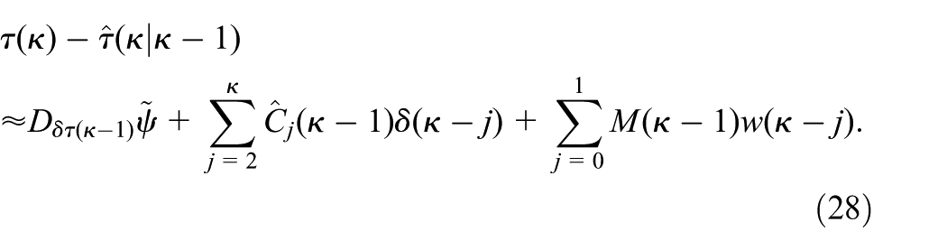
By neglecting higher-order terms, equation (27) can be approximated by
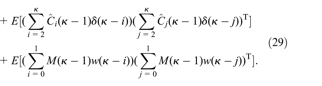
Let be the covariance matrix of estimation error by using (28), then is represented by
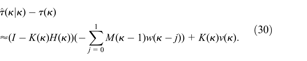
The estimation of the state vector is chosen as . Noting that with , the estimation error by supposing that holds is calculated by
For the case , we obtain
where and .
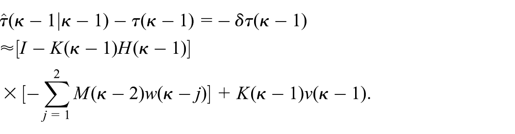
For the case , we give
Meanwhile, we have
Besides, we use equation (30) and replace with to obtain
Based on the definition of , we yield
From (34), we get
and
where .
It also has
Based on the covariance matrix of the process noise , it yields
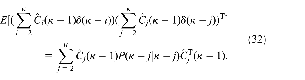
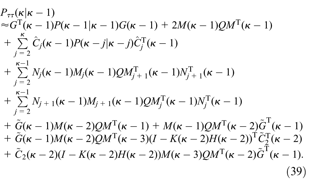
According to (32)–(38) and defining , is approximated by
Defining the following weights
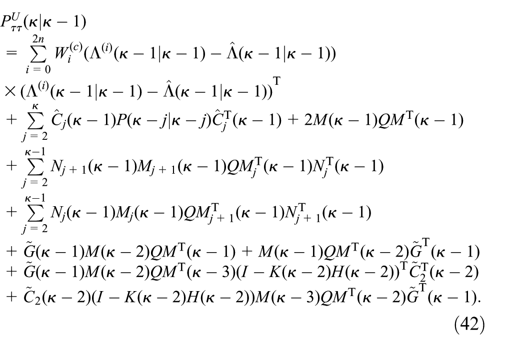
where is related with the probability distribution. For the normal distribution, we set . Therefore, based on , the prediction error matrix is obtained by
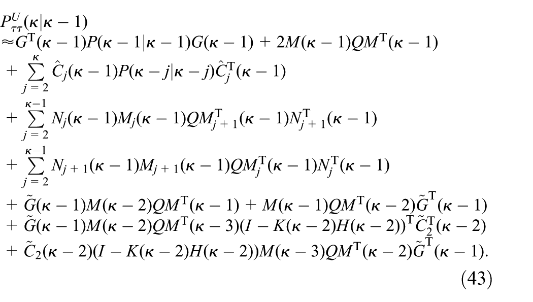
By using Appendix A, the predication error matrix is obtained by
Owing to (39) and (43), we can obviously know that the predication error matrix and are approximate. Thus, we can replace with .
Approximations of measurement output predication and predication error matrix
From (11), the predication is obtained as
The approximate predication error matrix is given by (42). According to the concept of U-T, the calculation method of the points considering the nonlinear function is given as follows
where .
We denote and with for . The measurement output can be represented by
The predication of the measurement output can be represented by
where .
Letting for and for , the predication of the measurement output for the th points is combined by (45) as
Obviously, the predication of the measurement and are the third-order approximations.
By using for , Appendix B and , the measurement error matrix is given by
where is the sum of the th order terms for with respect to .
From Appendix B, the measurement error matrix is derived by
where is the sum of the th order terms for with respect to .
Based on is the estimation error covariance matrix. Thus, becomes
where is the sum of the th order terms for with respect to .
By using , the error matrix is derived by
where is the sum of the th order terms for with respect to .
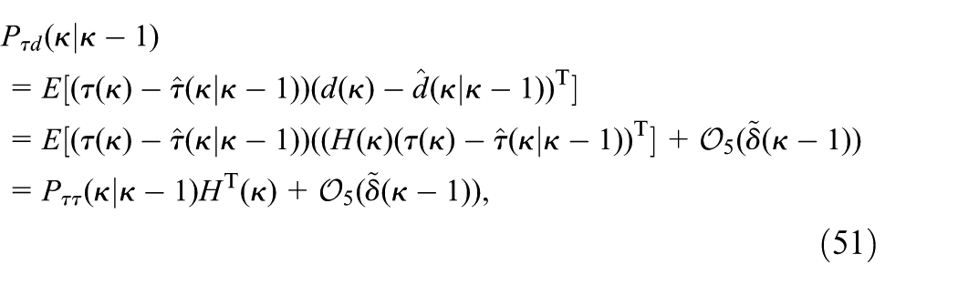
According to (49)–(52), the satisfactory approximation can be obtained by replacing and with and .
The Kalman gain matrix is determined by . Then, the updating equations for and the estimation error matrix are given by
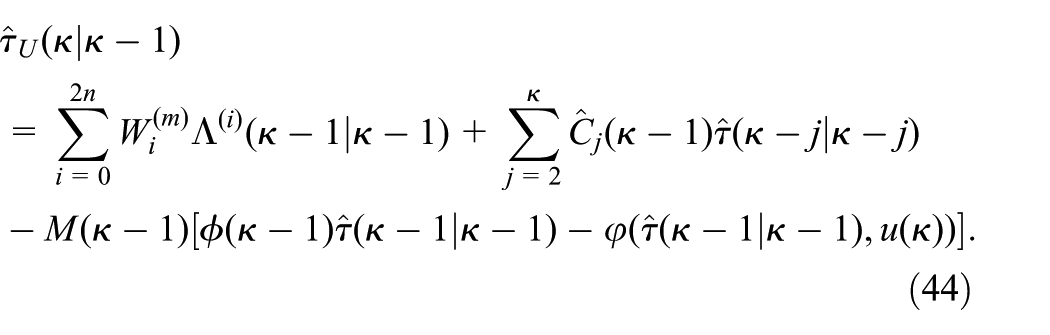
Remark 1: For the increase of index , the absolute value of the parameter becomes small rapidly. Hence, the predication of and for are calculated with the truncation to solve the limitation of storage space. The predication and the predication error matrix are written as follows
where .
Algorithm 1: The fractional-order HEUKFs for fractional-order nonlinear system (1) with the measurement output (2) for uncorrelated noises are divided into as the following steps.
Utilize the first-order Taylor expansion and U-T based on FOAD to obtain the system model difference equation.
Give the points for to get and by using (55) and (56).
Give the points for to obtain .
Calculate and based on (50) and (52).
Use the approximations of and to obtain the Kalman gain matrix .
Compute the state estimation and the estimation error matrix by using (53) and (54).
Simulation examples
A nonlinear fractional-order system involving process noise and measurement noise is presented as follows
where with the input frequency , and the initial state is . The measurement is selected as . The sampling period s and the running time 30s are set for this example. The sampling values of the noises and are white Gaussian noises with the covariance matrices and .
Select = 0.5, = 2, = 2 for the parameters of the fractional-order HEUKFs. The initial value of estimation vector and the error matrix are set as and respectively. In order to obtain more accurate error estimation
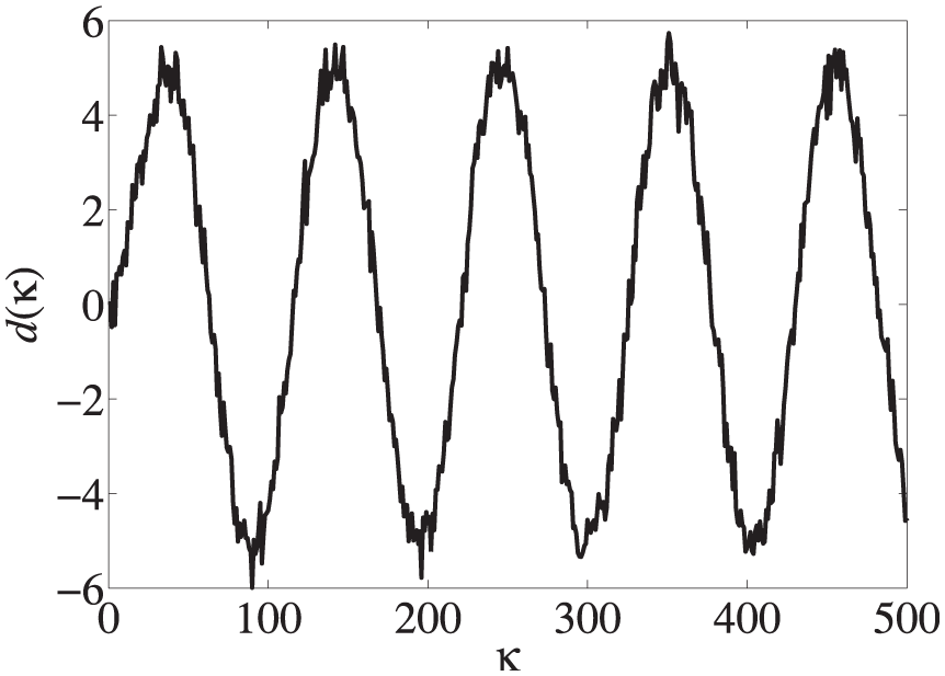
is defined as the error index, and the number of sampling values is . The simulation software is MATLAB 2009a, and the hardware configuration is Intel (R) Core (TM) i3-2350M, with the CPU processing speed of 2.30 GHz and 2 GB of RAM. The measurement with =500 is drawn in Figure 1.
Measurement in Example 1.
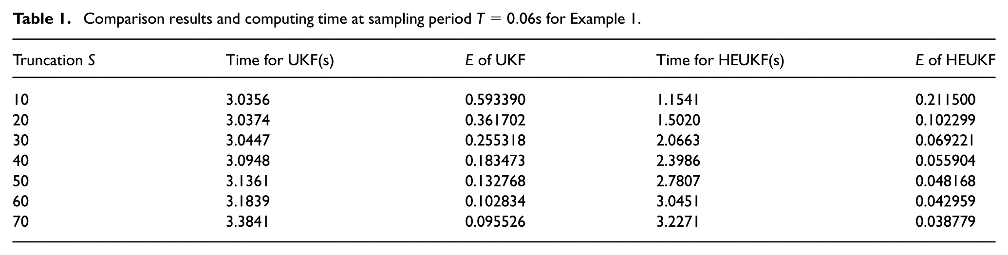
To determine the appropriate truncation , the parameters = 0.06s, = 0.8 and = 1 rad/s are selected. The comparison results and computing time with respect to the state estimation accuracy using the fractional-order HEUKF and UKF with different truncations are given in Table 1.
Comparison results and computing time at sampling period s for Example 1.
Truncation
Time for UKF(s)
of UKF
Time for HEUKF(s)
of HEUKF
10
3.0356
0.593390
1.1541
0.211500
20
3.0374
0.361702
1.5020
0.102299
30
3.0447
0.255318
2.0663
0.069221
40
3.0948
0.183473
2.3986
0.055904
50
3.1361
0.132768
2.7807
0.048168
60
3.1839
0.102834
3.0451
0.042959
70
3.3841
0.095526
3.2271
0.038779
From the results in Table 1, these conclusions can be drawn: As the truncation increases, the error index derived from the fractional-order HEUKF and the fractional-order UKF gradually becomes smaller. For each fixed truncation , the estimation error index using the fractional-order HEUKF is smaller than the corresponding one using the fractional-order UKF. Meanwhile, as the truncation increases, the computation time for the fractional-order UKF using GLD definition becomes longer compared with the fractional-order HEUKF using the FOAD. However, a larger truncation results in an increase of the computational burden. Therefore, it is necessary to choose a suitable truncation .
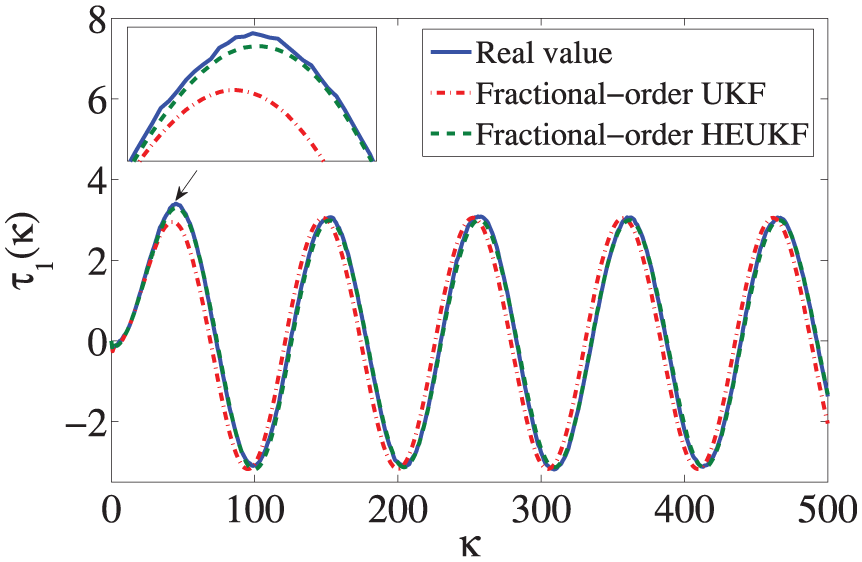
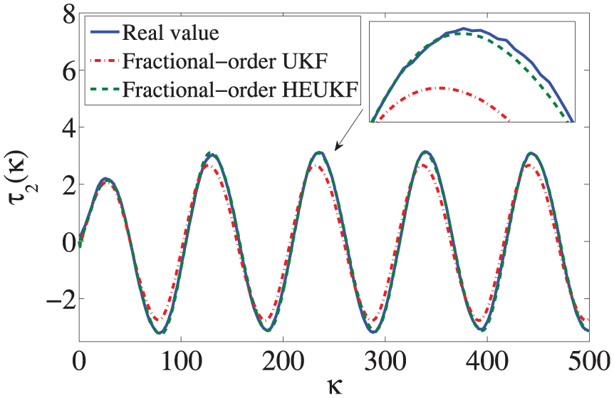
If the parameters = 30, = 0.8, = 1 rad/s and s are fixed, the error comparison results using the fractional-order HEUKF and UKF are shown in Figure 2 and Figure 3, respectively.
and its estimations in Example 1.
and its estimations in Example 1.
It can be seen from Figure 2 and Figure 3 that the responses obtained by the fractional-order HEUKF and the fractional-order UKF methods can estimate the dynamic responses of the fractional-order system in this example. But, the tracking effect produced by the proposed fractional-order HEUKF is better than the corresponding one using fractional-order UKF.
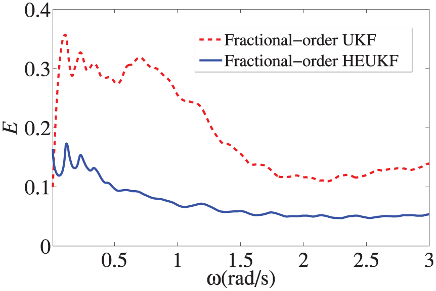
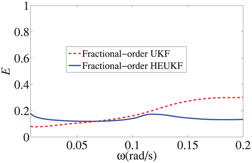
Meanwhile, the results of error index correspond to different frequencies using the fractional-order HEUKF and UKF are depicted in Figure 4 and Figure 5 with the truncation = 30, the sampling period = 0.06s and the order = 0.8.
Error indexes with different frequencies in Example 1.
Error indexes with the input signal different frequencies in Example 1.
Figure 4 shows the estimation error from the input signal frequency = 0.01 rad/s to 3 rad/s with the step 0.002 rad/s using the fractional-order HEUKF and the fractional-order UKF. Figure 5 shows the estimation error from the input signal frequency = 0.01 rad/s to 0.2 rad/s with the step 0.002 rad/s using the fractional-order HEUKF and the fractional-order UKF.
From the results in Figure 4 and Figure 5, these conclusions can be drawn: The UKF algorithm is better than the proposed HEUKF algorithm if the frequency in the input signal is small, which is shown in Figure 5; that is, the dynamic response of the nonlinear fractional-order system does not change significantly in a period. However, with the increase of input frequency , the index obtained by the HEUKF algorithm proposed in this paper is significantly smaller than that obtained by the UKF algorithm. This phenomenon shows that the HEUKF algorithm based on FOAD algorithm is more effective than UKF algorithm for estimating the nonlinear fractional-order system with obvious changes in a sampling period, which is also the advantage of FOAD algorithm. It can be seen from the comparison curves shown in Figure 4 that the fractional-order HEUKF with the increase of input frequency can obtain more accurate estimation results than the fractional-order UKF method for this example.
To compare the state estimation with different orders and different truncations , the parameters = 0.06s and = 1rad/s are selected. The accuracy comparison results of the state estimation using the fractional-order HEUKF and UKF with different orders and different truncations are given in Table 2 and Table 3.
Comparison results with different orders and truncations using fractional-order UKF for Example 1.
Order
=10
=20
=30
=40
=50
=60
=70
0.70
0.581189
0.366055
0.257556
0.182077
0.129360
0.098768
0.089721
0.75
0.596198
0.367925
0.257983
0.182842
0.129807
0.098712
0.090059
0.85
0.563275
0.345552
0.249679
0.185031
0.140111
0.114855
0.109606
0.90
0.490951
0.315858
0.240071
0.188056
0.152952
0.134760
0.131696
0.95
0.356141
0.264789
0.221202
0.189985
0.169920
0.160467
0.159182
Comparison results with different orders and truncations using fractional-order HEUKF for Example 1.
Order
=10
=20
=30
=40
=50
=60
=70
0.70
0.248477
0.127111
0.088710
0.071834
0.061153
0.053340
0.046864
0.75
0.233745
0.116660
0.080045
0.064458
0.055028
0.048389
0.043022
0.85
0.180100
0.084049
0.056598
0.046566
0.040905
0.037294
0.034298
0.90
0.138962
0.063806
0.044467
0.038566
0.035430
0.033394
0.031480
0.95
0.085110
0.042269
0.033966
0.032628
0.032015
0.031289
0.030353
Table 2 and Table 3 offer the comparison results of the state estimation using the fractional-order HEUKF and UKF with different truncations and different orders . For all of the orders , each estimation error index using the fractional-order HEUKF is smaller than the corresponding one using the fractional-order UKF. Therefore, the fractional-order HEUKF can achieve more accurate state estimation.
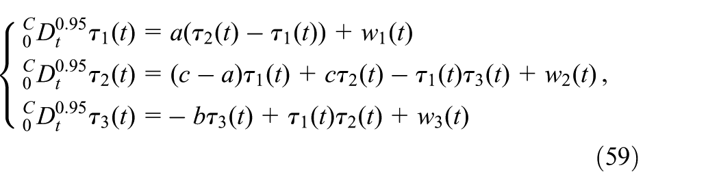
Example 2: Consider the following fractional-order Chen system in Gao et al. (2019) discussed as
where , and .
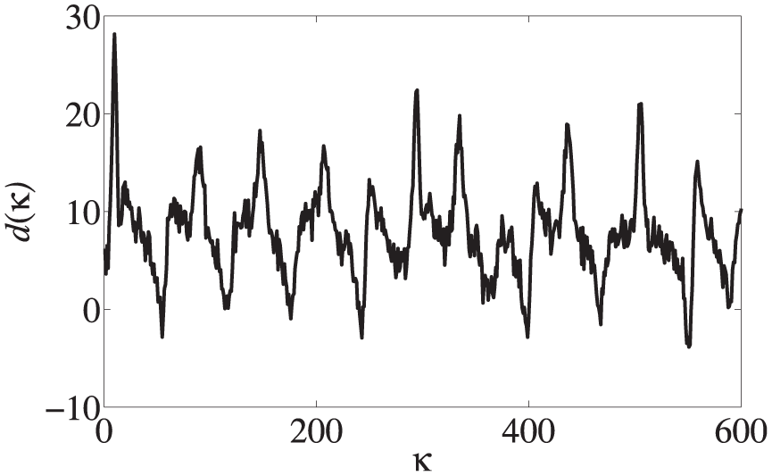
The initial state is . The measurement is chosen as . The sampling period s and the running time 30s are set for this example. The sampling values of the noises and are white Gaussian noises with the covariance matrices and . The parameters of the fractional-order HEUKF are selected = 0.5, = 2 and = 3. The initial values of estimation vector and the error matrix are set as and , respectively. Besides, the measurement with =600 is drawn in Figure 6.
Measurement in Example 2.
The comparison results and computing time using the fractional-order EKF and HEUKF with different truncations and sampling period s are given in Table 4.
Comparison results and computing time with sampling period s for Example 2.
Truncation
Time for EKF(s)
of EKF
Time for HEUKF(s)
of HEUKF
10
2.5122
0.230290
1.0629
0.129695
20
2.6455
0.196711
1.6580
0.080027
30
2.6855
0.190266
2.0995
0.067747
40
2.7116
0.187947
2.2448
0.063153
50
3.0076
0.187222
2.7120
0.061414
60
3.1125
0.186246
3.0242
0.060224
70
4.4726
0.185436
3.4120
0.059320
In Table 4, the comparison results demonstrate that the error index defined in (58) using the fractional-order EKF and HEUKF become smaller, as the truncation increases. Meanwhile, the computation time for the fractional-order EKF using GLD definition with increasing of truncation becomes longer compared with the fractional-order HEUKF using FOAD. Compared with the fractional-order EKF, the fractional-order HEUKF can improve the state estimation accuracy of fractional-order Chen system discussed in the example. Considering the estimation accuracy and the computational complexity, the truncation = 30 is suitable for this system.
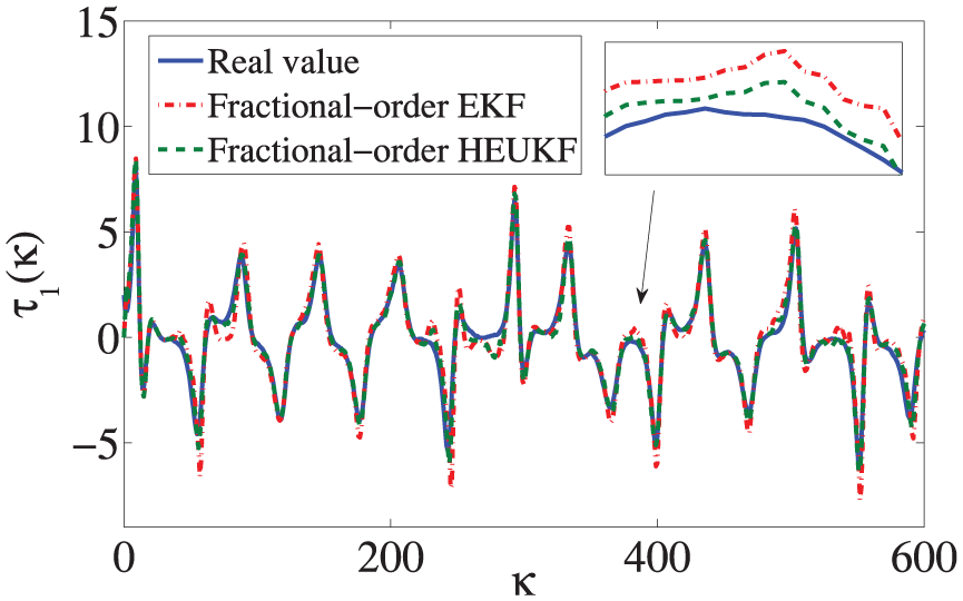
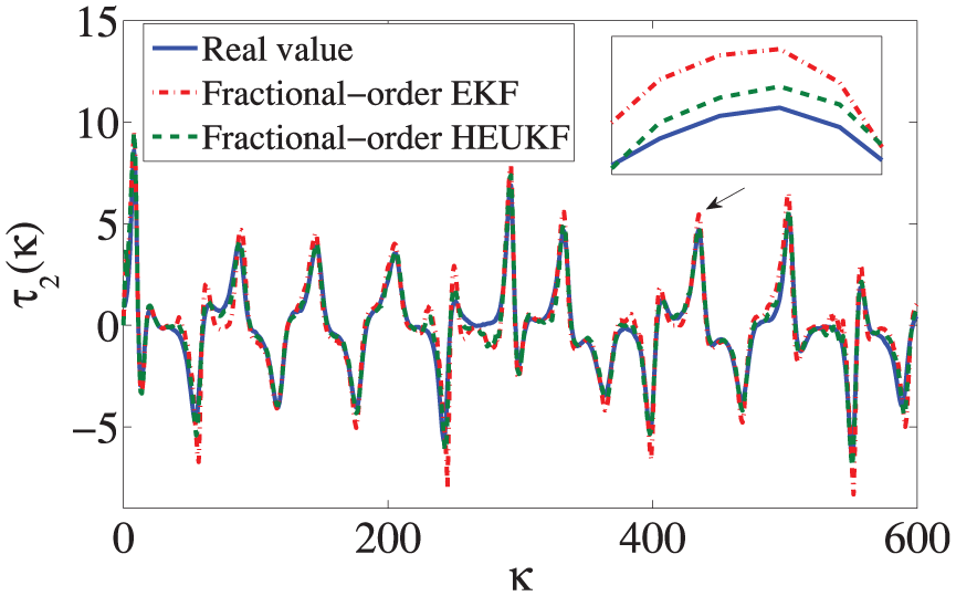
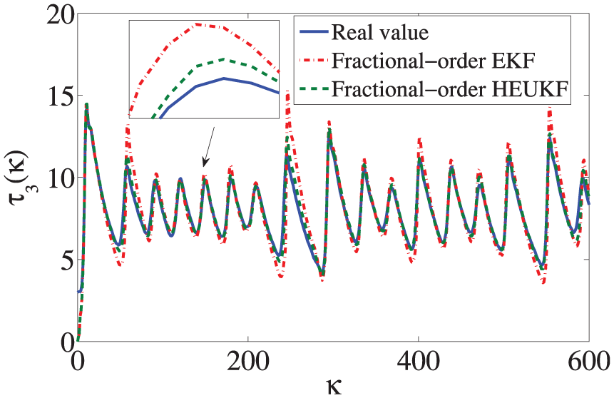
The estimation values of the state vector using fractional-order HEUKF and EKF with the truncation = 30 and the sampling period = 0.05s are shown in Figures 7–9.
and its estimations in Example 2.
and its estimations in Example 2.
and its estimations in Example 2.
From Figures 7–9, it can be seen that the studied fractional-order HEUKF can effectively track the dynamic behavior of the fractional-order Chen system involving process and measurement noises. Although the characteristics of the fractional-order Chen system as a strong nonlinear fractional-order system affect the dynamic behavior, the proposed the fractional-order HEUKF can still achieve the state estimation. Thus, the fractional-order HEUKF designed in this paper is a powerful state observer to improve the estimation accuracy involving process and measurement noises.
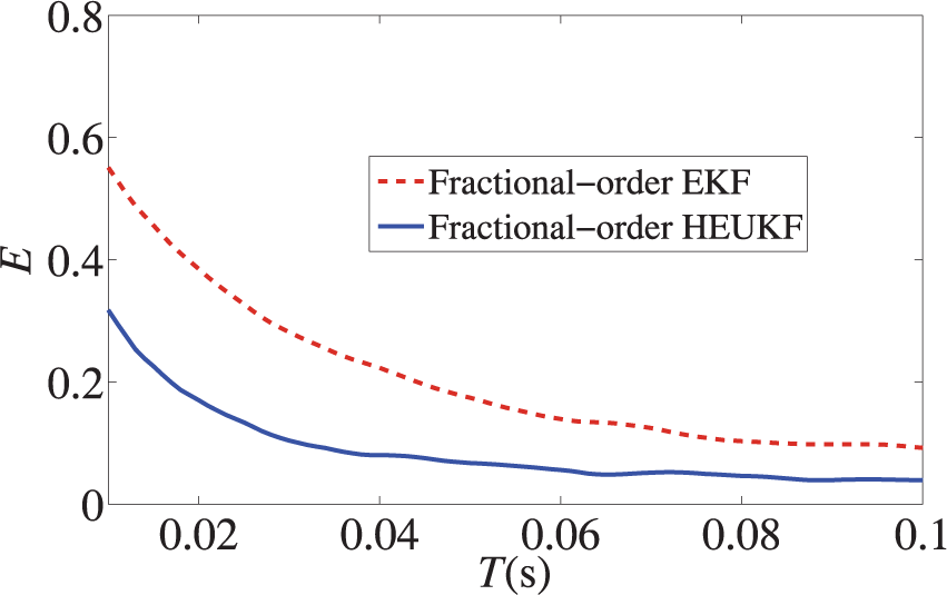
Meanwhile, the curves of error index correspond to different sampling periods with the truncation = 30 for the fractional-order EKF and the fractional-order HEUKF are depicted in Figure 10.
Error indexes with different sampling periods in Example 2.
Figure 10 shows the error indexes from = 0.01s to 0.1s with the step 0.001s using fractional-order HEUKF and EKF. For the selected sampling period, the error index produced by proposed fractional-order HEUKF is smaller than the corresponding one produced by the fractional-order EKF. Therefore, the fractional-order HEUKF is more suitable for the state estimation of the nonlinear system with strong nonlinearity.
Conclusion
In this paper, a HEUKF design method is proposed for the state estimation of continuous-time nonlinear fractional-order systems with process and measurement noises. The GLD definition and the FOAD method are used to obtain the system model with the difference equation description. The first-order Taylor expansion used in the EKF method is performed for a nonlinear function at the current time. Meanwhile, the U-T used in the UKF also focuses on the previous time nonlinear function. Based on the U-T concept, the Taylor expansion is applied to the nonlinear function at the points, and the theoretical basis of the third-order approximations of the nonlinear function is realized. Through numerical examples, we verify that the HEUKFs by FOAD is different from the UKF and EKF based on the GLD definition. Compared with the fractional-order EKF and UKF by using GLD definition, the proposed HEUKFs can effectively track the dynamic response of continuous-time nonlinear fractional-order systems. Therefore, the state estimation of the fractional-order nonlinear systems are completed, and the uncorrelated process and measurement noises problem are solved. In future work, the fractional-order Kalman filters to deal with some unknown parameters and correlated noises for the state estimation of the nonlinear fractional-order systems will be investigated.
Footnotes
Appendix A
Furthermore, from (16) and (21), the errors for and are yielded by
Appendix B
By using (46)–(48), we obtain the measurement error and as follows
and
Meanwhile, we have as follows
Declaration of conflicting interests
The author(s) declared no potential conflicts of interest with respect to the research, authorship, and/or publication of this article.
Funding
The author(s) disclosed receipt of the following financial support for the research, authorship, and/or publication of this article: This work was supported by Liaoning Revitalization Talents Program under Grant XLYC1807229, Liaoning University Science Research Fund LDGY2019020, Natural Science Foundation of Liaoning Province, China under Grant 20180520009 and China Postdoctoral Science Foundation Funded Project under Grant 2019M651206.
ORCID iD
Zhe Gao
References
1.
ChenCYDongWJDjapicV (2018) Distributed H-2/H filtering over infinite horizon. International Journal of Adaptive Control and Signal Processing32(2): 330–343.
2.
ChenYZhanmeiLV (2012) Positive solutions for fractional differential equations with variable coefficients. Electronic Journal of Differential Equations2012(80): 1–10.
3.
DongGZChenZHWeiJWLingQ (2018) Battery health prognosis using brownian motion modeling and particle filtering. IEEE Transactions on Industrial Electronics65(11): 8646–8655.
4.
GaoZ (2018) Kalman filters for continuous-time fractional-order systems involving fractional-order colored noises using Tustin Generating function. International Journal of Control Automation and System16(3): 1049–1059.
5.
GaoZLiuYTYangCChenXJ (2019) Unscended Kalman filter for continuous-time nonlinear fractional-order systems with process and measurement noises. Asian Journal of Control. DOI: 10.1002/asjc.2077.
6.
HamamciSE (2008) Stabilization using fractional-order PI and PID controllers. Nonlinear Dynamics51 (1–2): 329–343,.
7.
HeWWilliardNChenCCPechtM (2013) State of charge estimation for electric vehicle batteries using unscented Kalman filtering, Microelectronics Reliability53(6): 840–847.
8.
HuangLLBaleanuDMoZWWuGC (2018) Fractional discrete-time diffusion equation with uncertainty: Applications of fuzzy discrete fractional calculus. Physica A-Ststistical Mechanics and Its Applications508: 166–175.
9.
HuangSHZhouBLiCBWuQW (2018) Fractional-order modeling and sliding mode control of energy-saving and emission-reduction dynamic evolution system. International Journal of Electrical Power and Energy Systems100: 400–410.
10.
IonescuCLopesACopotD, et al. (2017) The role of fractional calculus in modeling biological phenomena: A review. Communications in Nonlinear Science and Numerical Simulation51: 141–159.
11.
LiGJCaoJDAlsaediAAhmadB (2018) Limit cycle oscillation in aeroelastic systems and its adaptive fractional-order fuzzy control. International Journal of Machine Learning and Cybernetics9(8): 1297–1305.
12.
LiuFHGaoZYangCMaRC (2019) Fractional-order Kalman filters for continuous-time fractional-order systems involving correlated and uncorrelated process and measurement noises. Transactions of the Institute of Measurement and Control41(7): 1933–1947.
13.
MachadoJATGalhanoAMTrujilloJJ (2014) On development of fractional calculus during the last fifty years. Scientometrics98(1): 577–582.
14.
MiaoZYShiHYZhangYXuF (2017) Neural network-aided variational Bayesian adaptive cubature Kalman filtering for nonlinear state estimation. Measurement Science and Technology28(10): 105003.
15.
NosratiKShafieeM (2018) Kalman filtering for discrete-time linear fractional-order singular systems. IET Control Theory and Applications12(9): 1254–1266.
RamezaniASafarinejadianB (2018) A modified fractional-order unscented Kalman filter for nonlinear fractional-order systems. Circuits Systems and Signal Processing37(9): 3756–3784.
18.
SadeghianHSalariehHAlastyAMeghdariA (2013) On the general Kalman filter for discrete time stochastic fractional systems. Mechatronics23(7): 764–771.
19.
SadeghzadehAMomeniH (2016) Robust output feedback control for discrete-time systems with ellipsoidal uncertainty. IMA Journal of Mathematical Control and Information33(4): 911–932.
20.
SafarinejadianBKianpourNMojtabaA(2018) State estimation in fractional-order systems with coloured measurement noise. Transactions of the Institute of Masurement and Control40(6): 1819–1835.
21.
SenthilRJanarthananKPrakashJ (2006) Nonlinear state estimation using fuzzy Kalman filter. Indutrial and Engineering Chemistry Research45(25): 8678–8688.
22.
SierociukDDzielinskiA (2006) Fractional Kalman filter algorithm for the states, parameters and order of fractional system estimation. International Journal of Applied Mathematics and Computer Science16(1): 129–140.
23.
SierociukDZiubinskiP (2014) Fractional order estimation schemes for fractional and integer order systems with constant and variable fractional order colored noise. Circuits, Systems and Signal Processing33(12): 3861–3882.
24.
SimonD (2010) Kalman filtering with state constraints: a survey of linear and nonlinear algorithms. IET Control Theory and Applications4 (8): 1303–1318.
25.
SunFCHuXSZouYLiSG (2011) Adaptive unscented Kalman filtering for state of charge estimation of a lithium-ion battery for electric vehicles. Energy36(5): 3531–3540.
26.
SunYHWuXPRajchakitGWeiZN (2017) Fractional extended Kalman filtering for non-linear fractional system with Lévy noises. IET Control Theory and Applications11(3): 349–359.
27.
TarasovVETarasovaVV (2018) Macroeconomic models with long dynamic memory: Fractional calculus approach. Applied Mathematics and Computation338: 466–486.
28.
WangJLWangJHZhangDXShaoXW (2018) Stochastic feedback based Kalman Filter for nonlinear continuous-discrete systems. IEEE Transactions on Automatic Control63(9): 3002–3009.
29.
XiaoMLZhangYBWangZHFuHM (2018) An adaptive three-stage extended Kalman filter for nonlinear discrete-time system in presence of unknown inputs. ISA Transactions75: 101–117.
30.
YangCGaoZLiuFH (2018) Kalman filters for linear continuous-time fractional-order systems involving coloured noises using fractional-order average derivative. IET Control Theory and Applications12(4): 456–465.
31.
YangCGaoZLiuFHMaRC (2019) Extended Kalman filters for nonlinear fractional-order systems perturbed by colored noises. ISA Transactions. DOI: 10.1016/j.isatra.2019.07.010.
32.
ZareiJTabatabaeiM (2018) Fractional order unknown input filter design for fault detection of discrete fractional order linear systems. Transactions of the Institute of Measurement and Control40(16): 4321–4329.
33.
ZhanTLiuXZ (2018) A new singular system approach to output feedback sliding mode control for fractional order nonlinear systems. Journal of the Franklin Institute-Engineering and Applied Mathematics355(14): 6746–6762.
34.
ZhangJFHeXZhouDH (2017) Robust optimal filtering for linear time-varying systems with stochastic uncertainties. IET Control Theory and Applications11(18): 3297–3304.
35.
ZhangLLiSZhangEZChenQW (2017) Robust measure of non-linearity-based cubature Kalman filter. IET Science Measurement and Technology11(7): 929–938.
36.
ZhangMNlinXZYinWQ (2013) An improved tuning method of fractional order proportional differentiation (FOPD) controller for the path tracking control of tractors. Biosystems Engineering116(4): 478–486.
37.
ZhouXHYangJZhouWETongDB (2017) Stability analysis based on partition trajectory approach for switched neural networks with fractional Brown noise disturbance. International Journal of Control90(10): 2165–2177.
38.
ZhuBChangLBXuJNZhaFLiJS (2018) Huber-based adaptive Unscented Kalman Filter with non-Gaussian measurement noise. Circuits Systems and Signal Processing3 (9): 3842–3861.