Sliding mode control revisited

Abstract

Controller design for nonlinear systems in its general form is complicated and an open problem. Finding a solution to this problem becomes more complicated when unwanted terms, such as disturbance, are taken into account. To provide a robust design for a subclass of nonlinear systems, sliding mode controllers (SMCs) are used. These controllers have a systematic design procedure and can reject bounded disturbances and at the same time guarantee stability. The guaranteed stability is achieved by separating system states into two parts and assuming that the input to state stability (ISS) condition holds for internal dynamics. This condition restricts the applicability of the SMC and limits the system performance when the controller is designed based on that. In order to remove this restriction and improve the performance, the ISS condition has been relaxed in this study. The relaxation is performed by redesigning SMCs based on suggested Lyapunov functions. The proposed idea insures global asymptotic stability of the closed loop system and is used to revise different well-known SMCs such as conventional SMC, terminal SMC, non-singular terminal SMC, integral SMC, super-twisting SMC, and super-twisting integral SMC. Comparisons between conventional and revised versions are made using simulation to demonstrate excellence of the revisited controllers.

Keywords

Sliding mode control terminal sliding mode control integral sliding mode control Lyapunov-based design super twisting sliding mode control

Introduction

A well-known method with robustness against bounded matched uncertainties is sliding mode control (SMC) (Khalil, 2002). The SMC has been extended in many ways; for example, output regulation using dynamic SMC is proposed in Lu et al. (1999), where authors estimate states to be used in the feedback function for multiple input multiple output systems. Although many SMCs have been proposed and used in a wide range of applications, these methods have their limitations and research on the SMC is still a hot topic (Asl et al., 2017; Ding and Li, 2017; Han et al., 2017; Shtessel et al., 2017).

In SMC, the finite time convergence to the sliding surface is an interesting feature. The finite time reaching phase of the SMC, minimum time controllers, and dead-beat strategy in digital control were motivations for the introduction and development of the finite time stability concept and finite time controllers (Bhat and Bernstein, 2000). The finite time stability increases the robustness of the system, and this became a motivation for the introduction of finite time SMCs such as terminal SMC (TSMC) (Zhihong et al., 1994), non-singular TSMC (NTSMC) (Feng et al., 2002), and super-twisting SMC (STSMC) (Moreno and Osorio, 2012). In addition, in integral SMC (ISMC), one can use a finite time nominal controller to render the finite time convergence for the system (Yu and Long, 2015).

Some versions of SMCs have specific drawbacks such as the chattering phenomenon. A remedy to the chattering phenomenon is usage of higher order SMC (HOSMC) techniques (Laghrouche et al., 2007; Levant, 2005). While HOSMCs have been successfully extended for different applications such as observers for multiple input multiple output (MIMO) systems (Fridman et al., 2008), their stability analysis could be tricky. For some HOSMCs, stability analysis is not Lyapunov based and finding Lyapunov functions to prove their stability is important (Moreno and Osorio, 2012).

The SMC is a powerful strategy and it is used in to address many problems despite its drawbacks. One of such problems is fault tolerant control in which the SMC has been widely used in observer design. For instance, sliding mode observer (SMO) is used in Li et al. (2014) for Markovian jump stochastic systems (MJS) to eliminate effects of sensor faults and disturbances. The SMO has been also used for MJS with time-delays (Yang et al., 2018). In order to eliminate the sliding surface switches, a reduced order SMO has been proposed in Yang et al. (2019) for MJS in case of sensor and actuator faults. Another SMO for MJS has been also designed in Yang et al. (2018), which eliminates sliding mode surface switches.

Recently, the research focus is more on applications of SMC while its classical core has remained untouched. The SMC scheme involves: (i) the selection of a hypersurface or a manifold (i.e. the sliding manifold) such that the system trajectory exhibits desirable behaviour when confined to this sliding manifold and (ii) finding feedback gains so that the system trajectory intersects and stays on the sliding manifold (Azar et al., 2015). Lyapunov stability analysis in the conventional SMC is divided into two successive steps: the reaching phase and the sliding phase. In the first phase, only finite time convergence to the sliding surface is considered and boundedness of other states, that is, internal dynamics, is not proved in the stability analysis. After finite time convergence of the first phase, the system stability is guaranteed using a Lyapunov function in the second phase. However, even when the sliding phase convergence is exponential, only local stability of the conventional SMC is guaranteed (Khalil, 2002). Global stability can only be guaranteed when the internal dynamics satisfies the input to state stability (ISS) condition. An attempt to relax the ISS condition is to define the sliding surface to be zero at the beginning, like how the sliding surface in the ISMC is defined. However, to be able to start on the sliding surface, the exact initial condition of the system is needed. Furthermore, a small perturbation can cause state deviation from the sliding surface. Therefore, it is not enough to start on the sliding surface in order to relax the ISS condition. For more details on stability analysis of the SMC, we refer to a survey that discusses available mathematical tools regarding stability, discontinuity of the right-hand side, and the ISS condition importance (Polyakov and Fridman, 2014).

To relax the ISS condition, we have proposed revised SMCs by guaranteeing the system stability in a single phase. The strategy is to consider a single Lyapunov function for the system stability analysis, which leads to a redesigned control signal. Consequently, the risk of finite escape time during the reaching phase will be eliminated without the ISS assumption. Not only does the proposed method guarantees the SMC global stability, but it also demonstrates more robustness against unexpected perturbations. Furthermore, the finite reaching time to the sliding surface holds, although it is not needed for the stability of the revised SMC versions.

The main novelty of this paper is relaxation of the ISS condition for the SMC by control redesign. Contributions of this paper are:

The ISS condition relaxation for the SMC;

Guaranteeing global asymptotic stability of the SMC;

Robustness improvement of the SMC using direct Lyapunov design;

Providing a framework to redesign all Lyapunov-based SMC schemes.

The rest of the paper is organized as follows. In the second section, the revised versions of SMC, TSMC, NTSMC, ISMC, STSMC, and STISMC are presented. In the third section, several numerical examples are provided to illustrate merits of the redesigned controllers. Finally, conclusions are drawn in the last section.

Main results

The main contribution of this paper is relaxation of the ISS condition in SMCs. In this section, we revise six SMC methods. The global asymptotic stability of each revised controller is proved using the Lyapunov theory.

SMC

Consider a nonlinear system presented in the regular form as

(\begin{matrix} \overset{\cdot}{η} \\ \overset{\cdot}{ζ} \end{matrix}) = (\begin{matrix} f_{a} (η, ζ) \\ f_{b} (η, ζ) + g (η, ζ) u + d (t) \end{matrix}),

(1)

where $(η, ζ) \in R^{n}$ is the system state, $u \in R^{p}$ is the system input, $d \in R^{p}$ is a bounded disturbance such that $d {(t)}_{\infty} < l$ , function $f_{a} (η, ζ)$ is continuously differentiable, and matrix $g (η, ζ)$ is non-singular and invertible. Furthermore, we assume that sliding surface s $(η, ζ) = ζ - ϕ (η)$ and radially unbounded Lyapunov candidate $V_{1} (η)$ exist such that $V_{1} (η)$ is a Lyapunov function when the sliding surface is reached, i.e., s $(η, ζ) = 0$ . Then, using the conventional SMC, the control law for system (1) is as

\begin{matrix} u (η, ζ) = - g^{- 1} (η, ζ) \\ (f_{b} (η, ζ) - \frac{\partial ϕ}{\partial η} f_{a} (η, ζ) + γ sign (s (η, ζ))), γ > l, \end{matrix}

(2)

where $γ$ is a constant scalar; see Khalil (2002) for more details. We note that u has the same dimension as $ζ$ and invertibility of $g (η, ζ)$ holds in practical systems. For instance, in single input systems, $g (η, ζ)$ is typically a non-zero constant number and therefore, invertible. In (2), function $sign (s)$ is considered as a vector whose i’th element is $sign (s_{i})$ .

In the conventional SMC, one cannot guarantee the global asymptotic stability of the system without additional assumptions. Even when the convergence to the sliding surface is finite time and it is exponential on the sliding surface, only the local stability is guaranteed Khalil (2002). In order to check the global asymptotic stability, we represent (1) as

(\begin{matrix} \overset{\cdot}{η} \\ \overset{\cdot}{s} \end{matrix}) = (\begin{matrix} f_{1} (η, s) \\ ν + d (t) \end{matrix}),

(3)

ν = - γ sign (s),

(4)

where $u (η, ζ) : = - g^{- 1} (η, ζ) (f_{b} (η, ζ) - \frac{\partial ϕ}{\partial η} f_{a} (η, ζ) - ν)$ and $f_{1} (η, s) : = f_{a} (η, s + ϕ (η))$ . Note that this transformation needs no condition other than invertibility of $g (η, ζ)$ . Note that function $f_{1} (η, s)$ is continuously differentiable and control signal $ν$ , defined in (4), is designed based on the conventional SMC. Lyapunov function $V_{1} (η)$ shows the asymptotic stability of the zero dynamics in (3), that is, $η$ ; the sliding surface s converges to zero in a finite time that implies that s is a vanishing input for the internal dynamics. Hence, the SMC method guarantees the global asymptotic stability of (3) if and only if the $η$ subsystem is input, that is, s, to state stable, that is, the ISS condition holds. The ISS condition for subsystem $η$ (t) with external input $ζ (t)$ , described in (1), is defined as

Definition 1: The subsystem $η$ with input $ζ$ is said to be input to state stable if there exists a class $K L$ function $α$ and a class $K$ function $β$ such that for any initial state $η (0)$ and any bounded input $ζ (t)$ , the solution $η (t)$ exists for all $t \geq 0$ and satisfies

‖ η (t) ‖ \leq α (‖ η (0) ‖, t) + β (sup_{0 \leq τ \leq t} ‖ ζ (τ) ‖) .

(5)

Inequality (5) guarantees that $η (t)$ remains bounded for any bounded input $ζ (t)$ . Furthermore, one can show that if $ζ (t)$ converges to zero as $t \to \infty$ , so does $η (t)$ (Khalil, 2002). Definition 1 implies the ISS condition does not hold for any unforced system, that is, when the input is zero, that is not globally stable. We refer to Sontag (2008) for more details on the ISS condition and its relevance to the control of practical systems.

In order to relax the ISS condition while assuring the global asymptotic stability, we combine the reaching and the sliding phases in the controller design as follows.

Theorem 1: Consider system (3) in which $f_{1} (η, s)$ is continuously differentiable and the radially unbounded Lyapunov function $V_{1} (η)$ exists that proves the system global asymptotic stability when s=0. Then, control law

ν = - γ_{2} \frac{\partial V_{1}}{\partial η} \bar{f} (η, s) - γ_{1} sign (s),

(6)

guarantees global asymptotic stability where function $\bar{f} (η, s)$ is defined such that

f_{1} (η, s) - f_{1} (η, 0) = diag {s_{1}, \dots, s_{p}} \bar{f} (η, s),

(7)

holds and $γ_{1} > l, γ_{2} > 0 .$

Proof: Since $f_{1} (η, s)$ is continuously differentiable, $\bar{f} (η, s)$ defined in (7) exists and is well-defined (Vidyasagar, 2002). Consider $V (η, s) = V_{1} (η) + \frac{1}{2 γ_{2}} s^{T} s$ as a Lyapunov candidate. The Lyapunov candidate derivative is as

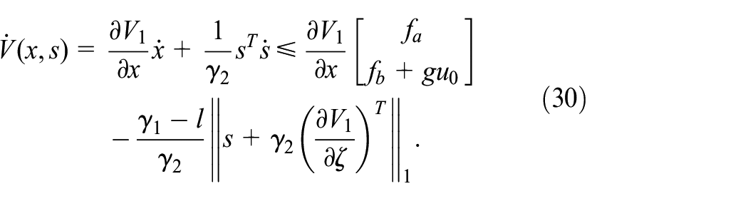
\overset{\cdot}{V} (η, s) = \frac{\partial V_{1}}{\partial η} f_{1} (η, s) + \frac{1}{γ_{2}} s^{T} \overset{\cdot}{s},

(8)

which in combination with (7) and (6) imply

\overset{\cdot}{V} (η, s) = \frac{\partial V_{1}}{\partial η} f_{1} (η, 0) + \frac{1}{γ_{2}} s^{T} (- γ_{1} sign (s) + d (t)) .

(9)

Since $‖ d (t) ‖_{\infty} < l$ , one can conclude

\overset{\cdot}{V} (η, s) \leq \frac{\partial V_{1}}{\partial η} f_{1} (η, 0) - \frac{γ_{1} - l}{γ_{2}} ‖ s ‖_{1} .

(10)

Since $V_{1} (η)$ guarantees the system stability when $s = 0$ , the term ${\overset{\cdot}{V}}_{1} (η) = \frac{\partial V_{1}}{\partial η} f_{1} (η, 0)$ is negative definite (ND) and as a result, $\overset{\cdot}{V} (η, s)$ is ND as well.

Remark 1: When $γ_{2} \to 0$ , the proposed control signal $ν$ , defined in (6), converges to its conventional version, that is, (4). Therefore, the proposed control law is a generalization of the conventional SMC and they are equivalent when $γ_{2} = 0$ . Nevertheless, the global asymptotic stability is guaranteed only when $γ_{2} > 0$ .

Remark 2: The control signal $ν$ , defined in (4), remains unchanged for all positive/negative s values. We suggest making the control signal dependent on the s value not only to guarantee the global stability but also to improve the transient behaviour of the system. Assuming $λ > 0$ , $ψ_{i} (0) = 0$ , and $s_{i} ψ_{i} (s_{i})$ for all $s_{i} \neq 0$ , adding the vector $- λ ψ (s)$ to the control signal improves the system convergence and the controller robustness specially when $ψ (s) \in K L_{\infty}$ . This additional term makes the Lyapunov function derivative more negative for both conventional and revised SMC methods.

Corollary 1: The revised SMC rejects any bounded matched disturbance with a known upper bound. Furthermore, the finite time convergence to the sliding surface in the revised SMC is preserved although it is not needed to prove the global asymptotic stability of the system.

Proof: The rejection of any bounded matched disturbance with a known upper bound is proved in Theorem 1. To prove the finite time convergence to the sliding surface, consider

V (s) = \frac{1}{2} s^{T} s,

(11)

\overset{\cdot}{V} (s) = - s^{T} (γ_{1} sign (s) - d (t) + γ_{2} \frac{\partial V_{1}}{\partial η} \bar{f} (η, s)) .

(12)

Assume $γ_{1} = l + \bar{l}$ with $\bar{l} > 0$ . According to Theorem 1, the system is globally asymptotically stable; hence, $\frac{\partial V_{1}}{\partial η} \bar{f} (η, s)$ converges to zero and

\exists T > 0 : \forall t > T \Rightarrow | γ_{2} \frac{\partial V_{1}}{\partial η} \bar{f} (η, s) | < \bar{l} - δ,

(13)

holds where $0 < δ < \bar{l}$ and $T < \infty$ . Consequently, the states are bounded for all $t \leq T$ and

t > T \Rightarrow \overset{\cdot}{V} (s) \leq - δ ‖ s ‖_{1},

(14)

holds. The Lyapunov function is second order and its derivative has a lower order, that is, one in this case, which implies s reaches zero in a finite time.

TSMC

In the terminal SMC, the conventional SMC is adjusted to get the finite time convergence for the system. Consider system (1) with $n = 2$ and $s = x_{2} + {kx}_{1}^{\frac{q}{p}}$ where k is a positive constant, and p and q are positive odd integers that satisfy $p > q$ .

According to the TSMC, the control input

\begin{matrix} u (x) = \frac{- 1}{β (x)} (α (x) + k \frac{q}{p} x_{1}^{\frac{q}{p} - 1} x_{2} + γ sign (s)), \\ γ > l, t_{r} \leq \frac{s (0)}{γ - l}, t_{s} = \frac{p}{k (p - q)} {| x_{1} (t_{r}) |}^{1 - \frac{q}{p}}, \end{matrix}

(15)

stabilizes

(\begin{matrix} {\overset{\cdot}{x}}_{1} \\ {\overset{\cdot}{x}}_{2} \end{matrix}) = (\begin{matrix} x_{2} \\ α (x) + β (x) u + d (t) \end{matrix}),

(16)

in a finite time (Feng et al., 2002). In (15), variables $t_{r}$ and $t_{s}$ are the surface reaching time and the system convergence after the reaching time, respectively. We revise the TSMC as follows.

Proposition 1: System (16) is globally asymptotically stable and it converges to zero in a finite time when the control input is designed as

u (x) = \frac{- 1}{β (x)} (α (x) + k \frac{q}{p} x_{1}^{\frac{q}{p} - 1} x_{2} + γ_{1} sign (s) + γ_{2} x_{1}),

(17)

Where $γ_{1} > l$ and $γ_{2} > 0$ .

Proof: Consider

V (x_{1}, s) = \frac{1}{2} x_{1}^{2} + \frac{1}{2 γ_{2}} s^{2},

(18)

as a Lyapunov candidate. The derivative of the sliding surface is

\overset{\cdot}{s} = α (x) + β (x) u + d (t) + k \frac{q}{p} x_{1}^{\frac{q}{p} - 1} x_{2} .

(19)

Using this derivative, one can conclude

\overset{\cdot}{V} \leq - {kx}_{1}^{1 + \frac{q}{p}} - \frac{γ_{1} - l}{γ_{2}} | s | .

(20)

Hence, the Lyapunov derivative is ND and the system is globally asymptotically stable. Proofs of the finite reaching time to the sliding surface and the system finite time stability on the surface are similar to the conventional TSMC (Feng et al., 2002).

Proposition 1 stated the global stability of the revised TSMC. In TSMC, state $x_{1}$ with a negative power is used in the controller which entails a singularity. The non-singular TSMC was proposed to solve this problem. Consider $s = x_{1} + \frac{1}{k} x_{2}^{\frac{p}{q}}$ as the sliding surface where $k > 0$ , $1 < \frac{p}{q} < 2$ , and p and q are positive odd integers. According to the NTSMC, control signal

u (x) = \frac{- 1}{β (x)} (α (x) + k \frac{q}{p} x_{2}^{2 - \frac{p}{q}} + γ sign (s)), γ > l,

(21)

stabilizes the system (16) in a finite time Feng, Y. et al, (2002). We revise the NTSMC as follows.

Proposition 2: System (16) is globally stable with the control input

u (x) = \frac{- 1}{β (x)} (α (x) + k \frac{q}{p} x_{2}^{2 - \frac{p}{q}} + γ_{1} sign (s) + γ_{2} x_{2}),

(22)

in a finite time when $γ_{1} > l$ and $γ_{2} > 0$ .

Proof: Consider the Lyapunov candidate

V (x_{1}, s) = \frac{1}{2} x_{1}^{2} + \frac{1}{2 γ_{2}} s^{2},

(23)

The sliding surface derivative is

\overset{\cdot}{s} = x_{2} + \frac{1}{k} \frac{p}{q} x_{1}^{\frac{p}{q} - 1} (α (x) + β (x) u + d (t)),

(24)

using which one can conclude

\overset{\cdot}{V} \leq - \frac{1}{k} {(ks - k x_{1})}^{1 + \frac{q}{p}} - \frac{γ_{1} - l}{γ_{2}} | s | .

(25)

Therefore, the Lyapunov derivative is ND and the system is globally asymptotically stable. The finite time convergence to the sliding surface and the finite time stability of the system is similar to the conventional NTSMS (Feng et al., 2002).

ISMC

The ISMC is a creative strategy to eliminate a few drawbacks of the conventional SMC. This controller rejects any bounded matched disturbance with a discontinuous control signal similar to the SMC. Unlike the SMC, the ISMC starts on the sliding surface and $s = 0$ at the beginning which implies global asymptotic stability. Furthermore, any control law that stabilize the nominal system can be used in the ISMC as the nominal controller, that is, the ISMC compensates the disturbance effects and uses the nominal controller to stabilize the nominal system.

Consider system (1) with $u_{0} (x)$ as its nominal controller and assume that Lyapunov function $V_{1} (x)$ proves the asymptotic stability of the nominal system using the nominal controller. The ISMC suggests

\begin{matrix} u (x) = u_{0} (x) - γ g^{- 1} sign (s), \\ s = ζ (t) - ζ (0) - \int_{0}^{t} (f_{b} (η, ζ) + g (η, ζ) u_{0} (x)) d t, \end{matrix}

(26)

as the control input and the sliding surface, respectively. This feedback law guarantees the system stability in the presence of bounded disturbance $d (t)$ (Utkin and Shi, 1996). One can see that $s (0) = 0$ by construction; in fact, s is a measure indicating the deviation of $ζ (t)$ from its nominal trajectory. Hence, staying on the sliding surface implies the disturbance effects on the system is rejected. Despite the ISMC merits, it uses the initial condition of the system in the sliding surface definition which might not be available. Consequently, the reaching phase might still exist, and the system stability analysis would rely on the ISS condition. We revise the ISMC as follows.

Proposition 3: Assume that function $f_{a} (η, ζ)$ in (1) is continuously differentiable and radially unbounded.

Lyapunov function $V_{1} (x)$ exists that proves the nominal system stability, i.e., when $d (t) = 0$ and $u (x) = u_{0} (x)$ . Then, system (1) is globally asymptotically stable using the control input

u (x) = u_{0} (x) - γ_{1} g^{- 1} sign (s + γ_{2} {(\frac{\partial V_{1}}{\partial ζ})}^{T}),

(27)

when $γ_{1} > l$ and $γ_{2} > 0$ .

Proof: Consider

V (x_{1}, s) = V_{1} (x) + \frac{1}{2 γ_{2}} s^{T} s,

(28)

as the Lyapunov candidate. The sliding surface derivative is

\overset{\cdot}{s} = - γ_{1} sign (s + γ_{2} {(\frac{\partial V_{1}}{\partial ζ})}^{T}) + d (t),

(29)

using which one can conclude

\begin{matrix} \overset{\cdot}{V} (x, s) = \frac{\partial V_{1}}{\partial x} \overset{\cdot}{x} + \frac{1}{γ_{2}} s^{T} \overset{\cdot}{s} \leq \frac{\partial V_{1}}{\partial x} [\begin{matrix} f_{a} \\ f_{b} + g u_{0} \end{matrix}] \\ - \frac{γ_{1} - l}{γ_{2}} ‖ s + γ_{2} {(\frac{\partial V_{1}}{\partial ζ})}^{T} ‖_{1} . \end{matrix}

(30)

The first term in the upper bound of $\overset{\cdot}{V} (x, s)$ is the Lyapunov derivative of the nominal system which was assumed to be ND; consequently, V $(x, s)$ is also ND and the system is globally asymptotically stable.

STSMC

The control signals in the introduced SMC methods are discontinuous, which result in the so-called chattering phenomenon. Higher order SMC algorithms were proposed to eliminate the chattering phenomenon. When discontinuity occurs in the n’th derivative of the sliding surface s, the design order is $n - 1$ and when $n \geq 2$ , the method is called a higher order SMC in which the chattering phenomenon does not appear in the sliding surface. Discontinuity of the control signal is another issue of the SMCs that one might hope to overcome using higher order SMCs. Nevertheless, usage of a higher order SMC does not imply that the control signal is continuous. In fact, the control signal cannot be continuous and reject any bounded disturbance at the same time unless the disturbance derivative would also be bounded. Even when the disturbance derivative is bounded, the control signal might be discontinuous in some higher order SMC methods such as the twisting SMC (Bartolini et al., 2003).

Assume the disturbance and its derivative values are bounded, then the STSMC method has a second order sliding surface and its control signal is continuous. Consider system (3) and assume $d (t)$ is bounded, $| \overset{\cdot}{d} (t) | < l$ , and radially unbounded Lyapunov function $V_{1} (η)$ exists that proves the system stability when $s (t) = 0$ and $d (t) = 0$ . Then, the STSMC suggests

\begin{matrix} ν = - γ_{1} \sqrt{| s |} sign (s) + ρ, \\ \overset{\cdot}{ρ} = - γ_{2} sign (s), \end{matrix}

(31)

as the control law. In (31), $ρ$ is the estimation of $- d (t)$ and the STSMC guarantees the system stability for some $γ_{1}$ and $γ_{2}$ , see Moreno and Osorio (2012), such as

γ_{1} = κ \sqrt{\frac{2 γ l}{(1 - β) α}}, γ_{2} = (\frac{1 + β}{1 - β}) l,

(32)

where

α = \frac{β γ - 1}{γ (1 - β^{2})}, κ = \frac{γ + β (β γ - 2)}{γ (1 - β^{2})}, 0 < β < 1, \frac{1}{β} < γ,

(33)

The STSMC asymptotic stability can be proved using Lyapunov method; for example, see Moreno and Osorio (2012). Define $z : = ρ + d (t)$ , and $ξ^{T} : = [\begin{matrix} \sqrt{| s |} sign (s) & z \end{matrix}]$ consider $V_{2} (ξ) = ξ^{T} P ξ$ as a Lyapunov function with a PD matrix P. Then

\overset{\cdot}{ξ} = \frac{1}{ξ_{1}} A ξ + [\begin{matrix} 0 \\ \overset{\cdot}{d} (t) \end{matrix}], A = [\begin{matrix} - \frac{1}{2} γ_{1} & \frac{1}{2} \\ - γ_{2} & 0 \end{matrix}],

(34)

holds and

{\overset{\cdot}{V}}_{2} (ξ) \leq - {| ξ_{1} |}^{- 0.5} ξ^{T} Q ξ,

(35)

shows the system stability where Q is a PD matrix. For instance, such P and Q matrices could be

P = [\begin{matrix} 1 & - \sqrt{\frac{(1 - β) α}{2 l γ}} \\ - \sqrt{\frac{(1 - β) α}{2 l γ}} & \frac{(1 - β) α}{2 l} \end{matrix}],

(36)

Q = [\begin{matrix} γ_{1} + 2 P_{12} (γ_{2} + l) + 2 l (1 - γ_{1} P_{12}) \frac{P_{22}}{P_{12}} - \frac{1}{2} (1 - γ_{1} P_{12}) + (γ_{2} + l) P_{22} \\ - \frac{1}{2} (1 - γ_{1} P_{12}) + (γ_{2} + l) P_{22} - P_{12} \end{matrix}],

(37)

where $P_{22} : = P (i, j)$ . Although the STSMC does not have some of the drawbacks of the SMC, the system convergence is not guaranteed during the reaching phase. The revised STSMC eliminates this issue and guarantees global asymptotic stability regardless of the ISS condition.

Proposition 4: Consider the conventional STSMC assumptions and $V_{1} (η)$ as a radially unbounded Lyapunov function that proves system (3) stability when $s = 0$ . Then, the system is globally asymptotically stable using

\begin{matrix} ν = - γ_{1} \sqrt{| s |} sign (s) + ρ + u_{m}, \\ \overset{\cdot}{ρ} = - γ_{2} sign (s) + u_{b}, \\ u_{m} = \frac{- P_{22}}{P_{11} P_{22} - P_{12}^{2}} \frac{\partial V_{1}}{\partial η} | s | \bar{f} (η, s), \\ u_{b} = \frac{P_{12}}{2 P_{11} P_{22} - 2 P_{12}^{2}} \frac{\partial V_{1}}{\partial η} \sqrt{| s |} \bar{f} (η, s), \end{matrix}

(38)

as the control law.

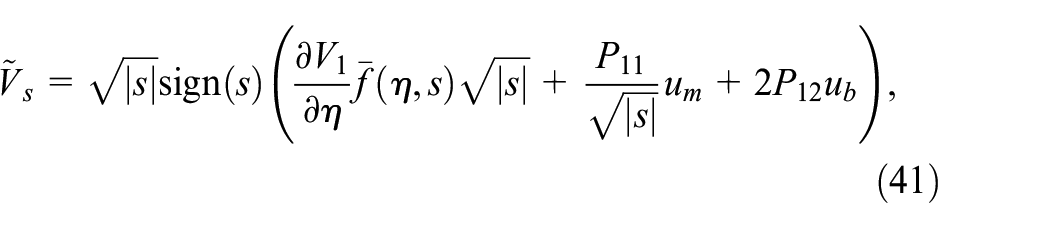
Proof: Assume $z : = ρ + d (t)$ , $V (η, ξ) = V_{1} (η) + V_{2} (ξ)$ , and $ξ^{T} : = [\begin{matrix} \sqrt{| s |} sign (s) & z \end{matrix}]$ . Then

\overset{\cdot}{V} (x, ξ) \leq \frac{\partial V_{1}}{\partial η} \bar{f} (η, 0) - {| ξ_{1} |}^{- 0.5} ξ^{T} Q ξ + {\tilde{V}}_{z} + {\tilde{V}}_{s},

(39)

{\tilde{V}}_{z} = z (\frac{P_{12}}{\sqrt{| s |}} u_{m} + 2 P_{22} u_{b}),

(40)

{\tilde{V}}_{s} = \sqrt{| s |} sign (s) (\frac{\partial V_{1}}{\partial η} \bar{f} (η, s) \sqrt{| s |} + \frac{P_{11}}{\sqrt{| s |}} u_{m} + 2 P_{12} u_{b}),

(41)

holds where $f_{1} (η, s) - f_{1} (η, 0) = s \bar{f} (η, s)$ . Substitution of $u_{m}$ and $u_{b}$ , defined in (38), in the Lyapunov function derivative implies ${\tilde{V}}_{z} = {\tilde{V}}_{s} = 0$ . Since $\frac{\partial V_{1}}{\partial η} \bar{f} (η, 0)$ is ND, the Lyapunov function derivative is also ND. This implies that the system is globally asymptotically stable.

STISMC

Consider system (1) and assume $u \in R$ and $| \frac{d}{d t} (\frac{d (t)}{g (x)}) | < l$ . In addition, assume that a nominal controller $u_{0} (x)$ and a Lyapunov function $V_{1} (x)$ exist such that $V_{1} (x)$ proves stability of the nominal system with the nominal controller. Then, the STISMC guarantees the system stability when

\begin{matrix} u (x) = u_{0} (x) + \frac{1}{g (x)} (- γ_{1} \sqrt{| s |} sign (s) + ρ), \\ s = x_{n} (t) - x_{n} (0) - \int_{0}^{t} (f_{b} (x) + g (x) u_{0} (x)) d t, \\ \overset{\cdot}{ρ} = - γ_{2} sign (s), \end{matrix}

(42)

is used. In (42), $γ_{1}$ and $γ_{2}$ are defined as in (32) and $ρ$ is estimation of $- d (t)$ . The system stability using the STISMC is proved using the Lyapunov function $V_{2} (ξ) = ξ^{T} P ξ$ and similar to the STSMC method.

The STISMC method uses the system initial condition in definition of the sliding surface which might not be available at the beginning; therefore, the reaching phase to the sliding surface still exists and the ISS condition is necessary for the global stability of the system. The revised STISMC eliminates this issue and guarantees the system stability, whether the system is on the sliding surface at the beginning or not.

Proposition 5: Consider the conventional STISMC assumptions on the system (1), nominal control law $u_{0} (x)$ , and $V_{1} (x)$ as a radially unbounded Lyapunov function that proves nominal system stability. Then, the system is globally asymptotically stable using

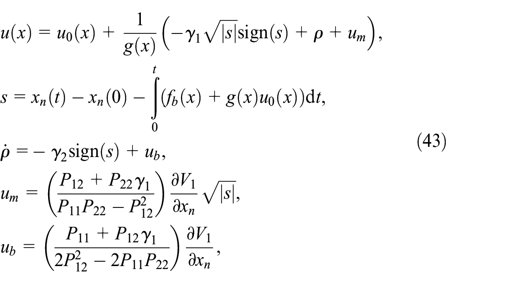
\begin{matrix} u (x) = u_{0} (x) + \frac{1}{g (x)} (- γ_{1} \sqrt{| s |} sign (s) + ρ + u_{m}), \\ s = x_{n} (t) - x_{n} (0) - \int_{0}^{t} (f_{b} (x) + g (x) u_{0} (x)) d t, \\ \overset{\cdot}{ρ} = - γ_{2} sign (s) + u_{b}, \\ u_{m} = (\frac{P_{12} + P_{22} γ_{1}}{P_{11} P_{22} - P_{12}^{2}}) \frac{\partial V_{1}}{\partial x_{n}} \sqrt{| s |}, \\ u_{b} = (\frac{P_{11} + P_{12} γ_{1}}{2 P_{12}^{2} - 2 P_{11} P_{22}}) \frac{\partial V_{1}}{\partial x_{n}}, \end{matrix}

(43)

as the new control law.

Proof: $z : = ρ + d (t)$ , $V (x, ξ) = V_{1} (x) + V_{2} (ξ)$ , and $ξ^{T} : = [\begin{matrix} \sqrt{| s |} sign (s) & z \end{matrix}]$ . Then

\overset{\cdot}{V} (x, ξ) \leq \frac{\partial V_{1}}{\partial x} [\begin{matrix} f_{a} \\ f_{b} + g u_{0} \end{matrix}] - {| ξ_{1} |}^{- 0.5} ξ^{T} Q ξ + {\tilde{V}}_{z} + {\tilde{V}}_{s},

(44)

{\tilde{V}}_{z} = z (\frac{\partial V_{1}}{\partial x_{n}} + \frac{P_{12}}{\sqrt{| s |}} u_{m} + 2 P_{22} u_{b}),

(45)

{\tilde{V}}_{s} = \sqrt{| s |} sign (s) (- γ_{1} \frac{\partial V_{1}}{\partial x_{n}} + \frac{P_{11}}{\sqrt{| s |}} u_{m} + 2 P_{12} u_{b}),

(46)

holds. Substitution of the $u_{m}$ and $u_{b}$ implies ${\tilde{V}}_{z} = {\tilde{V}}_{s} = 0$ . Therefore, the Lyapunov function derivative is ND and the system is globally asymptotically stable.

Remark 3: The conventional SMCs have been used successfully in the literature. Nevertheless, the conventional SMCs have been used either to provide local stability or in cases that ISS condition holds. Note that the ISS condition might or might not hold for a system based on the sliding surface definition. While the ISS condition does not hold in all cases, it inherently holds in ISMC and STISMC cases due to their sliding surface definition. Therefore, the revised ISMC and STISMC, with respect to their conventional versions, might just improve the transient behaviour of the system. Nevertheless, as we show next, one can come up with cases for which the revised SMC and STSMC stabilize the system while the conventional versions do not.

Numerical simulations

This section is devoted to provide numerical examples to illustrate merits of the revised controllers over their conventional counterparts.

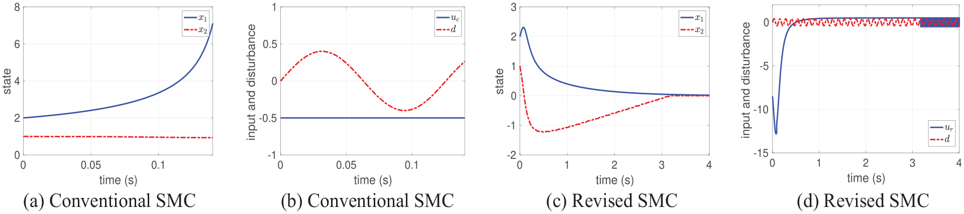
Example 1: Conventional versus revised SMC: Consider

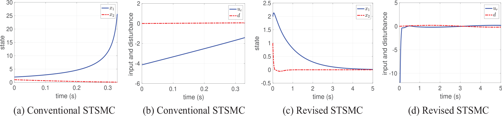
(\begin{matrix} {\overset{\cdot}{x}}_{1} \\ {\overset{\cdot}{x}}_{2} \end{matrix}) = (\begin{matrix} - x_{1} + x_{2} x_{1}^{3} \\ u + d (t) \end{matrix}),

(47)

where $x_{1}$ and $x_{2}$ are system states, u is the control signal, and $d (t) = 0.4 \sin (50 t)$ is the unknown, bounded disturbance. Consider the sliding surface as $s = x_{2}$ and the control input as $u : = u_{c} = - γ sign (s)$ , which are designed based on the conventional SMC. The Lyapunov function $V_{1} (x_{1}) = \frac{1}{2} x_{1}^{2}$ can be used to show the system stability when $s = 0$ . Likewise, the Lyapunov function $V_{2} (s) = \frac{1}{2} s^{2}$ can be used to prove finite reaching time when $γ > | d (t) |$ . According to Theorem 1, the revised control law would be $: = u_{r} = - γ_{1} sign (s) - x_{1}^{3}$ when $γ_{2} = 1$ and $γ_{1} = γ$ . The simulation results are presented in Figure 1. Sub-figure 1(a) shows $x_{1}$ goes to infinity, which implies that the conventional SMC might not be globally stable without the ISS condition; in contradiction, sub-figure 1(c) demonstrates that the revised method stabilizes the system.

Figure 1.

Simulation of the conventional and revised SMC for Example 1.

In Example 1, the conventional SMC is not globally stable. In fact, in this case, $x_{1} (t)$ has a finite escape time and it goes to infinity before $s = 0$ can be achieved. On the other hand, the system is globally asymptotically stable using the revised SMC.

Example 2: Conventional versus revised STSMC: Consider system (47) given in Example 1 with $d (t) = 0.2 \sin (t)$ and consider $s = x_{2}$ as the sliding surface. Using the conventional STSMC, the designed controller is

u_{c} = - γ_{1} \sqrt{| s |} sign (s) + ρ_{c},

(48)

{\overset{\cdot}{ρ}}_{c} = - γ_{2} sign (s) .

(49)

Consider Lyapunov function $V_{1} (x_{1}) = \frac{1}{2} x_{1}^{2}$ , which can be used to prove the system stability when $s = 0$ . Based on Proposition 4, the revised control signal is

u_{r} = - γ_{1} \sqrt{| s |} sign (s) + ρ_{r} + u_{m},

(50)

{\overset{\cdot}{ρ}}_{r} = - γ_{2} sign (s) + u_{b},

(51)

u_{m} = \frac{- P_{22}}{P_{11} P_{22} - P_{12}^{2}} x_{1}^{4} | s |,

(52)

u_{b} = \frac{P_{12}}{2 P_{11} P_{22} - 2 P_{12}^{2}} x_{1}^{4} \sqrt{| s |} .

(53)

By choosing $β = 0.5$ and $γ = 4$ , one can compute

P = [\begin{matrix} 1 & - 0.3227 \\ - 0.3227 & 0.4167 \end{matrix}], γ_{1} = 4.1312, γ_{2} = 0.6 .

(54)

Simulation results are given in Figure 2 for the conventional and the revised STSMC. State $x_{1}$ in sub-figure 2(a) goes to infinity, and this example shows that the conventional STSMC might not be globally stable. In contradiction, states converge to zero in the revised STSMC case, as shown in sub-figure 2(c).

Figure 2.

Simulation of the conventional and revised STSMC for Example 2.

Example 3: Conventional versus revised ISMC: Consider system (47) given in Example 1 with $d (t) = 0.2 \sin (t)$ . The conventional ISMC can be designed as

u (x) = u_{0} (x) - sign (s (t)),

(55)

u_{0} (x) = - x_{2} + x_{1}^{2} - x_{1}^{4} - 2 x_{1}^{4} x_{2},

(56)

s (t) = x_{2} (t) - x_{2} (0) - \int_{0}^{t} u_{0} (x) d t,

(57)

On the other hand, the revised ISMC, see (27), can be designed as

u (x) = u_{0} (x) - sign (s (t) + 100 (x_{2} + x_{1}^{2})),

(58)

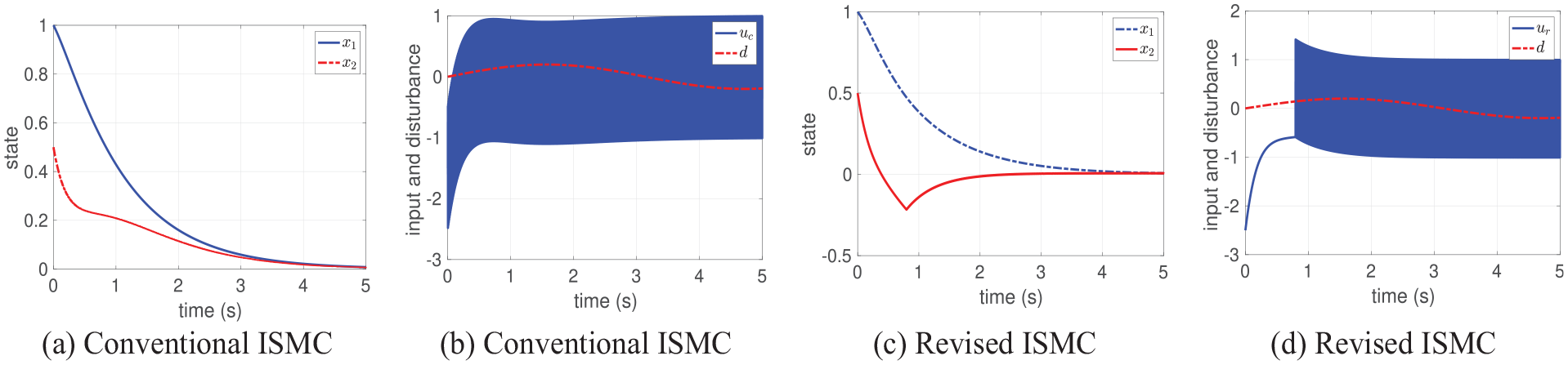
The simulation results are presented in Figure 3. ISMC satisfies the ISS condition by design and therefore, both conventional and revised ISMC are stable. Nevertheless, the figure shows that the revised ISMC has a better transient behaviour.

Figure 3.

Simulation of the conventional and revised ISMC for Example 3.

Example 4: Conventional versus revised STISMC: Consider system (47) given in Example 1 with $d (t) = 0.2 \sin (t)$ . The conventional STISMC can be designed as

u (x) = u_{0} (x) - 4.13 \sqrt{| s |} sign (s) + ρ (t),

(59)

u_{0} (x) = - x_{2} + x_{1}^{2} - x_{1}^{4} - 2 x_{1}^{4} x_{2},

(60)

s (t) = x_{2} (t) - x_{2} (0) - \int_{0}^{t} u_{0} (x) d t,

(61)

\overset{\cdot}{ρ} (t) = - 0.6 sign (s (t)),

(62)

On the other hand, the revised STISMC, see (43), can be designed as

u (x) = u_{0} (x) - 4.13 \sqrt{| s |} sign (s) + ρ (t) + 0.3 (x_{2} + x_{1}^{2}) \sqrt{| s |},

(63)

\overset{\cdot}{ρ} (t) = - 0.6 sign (s (t)) - 1.08 (x_{2} + x_{1}^{2}),

(64)

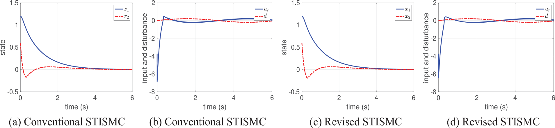
Since the sliding surface is zero initially, both simulations provide almost the same results. In order to see some difference, let us assume that $x_{2} (0)$ has been replaced by zero in (61), that is, the initial condition of the sliding surface has changed to a nonzero value. The simulation results are presented in Figure 4.

Figure 4.

Simulation of the conventional and revised STISMC for Example 4.

STISMC satisfies the ISS condition by design and therefore, both conventional and revised STISMC are stable. Nevertheless, the figure shows that the revised STISMC has a better transient behaviour.

Example 5: Conventional versus revised TSMC: Consider

(\begin{matrix} {\overset{\cdot}{x}}_{1} \\ {\overset{\cdot}{x}}_{2} \end{matrix}) = (\begin{matrix} x_{2} \\ u + d (t) \end{matrix}),

(65)

with $d (t) = 0.4 \sin (t)$ . The designed controller signal based on the conventional TSMC, as in (15), is

u (x) = - sign (s) - x_{1}^{- \frac{2}{3}} x_{2},

(66)

s (t) = x_{2} + 3 x_{1}^{\frac{1}{3}} .

(67)

On the other hand, the designed revised TSMC, as in (17), is

u (x) = - sign (s) - x_{1}^{- \frac{2}{3}} x_{2} - 3 x_{1},

(68)

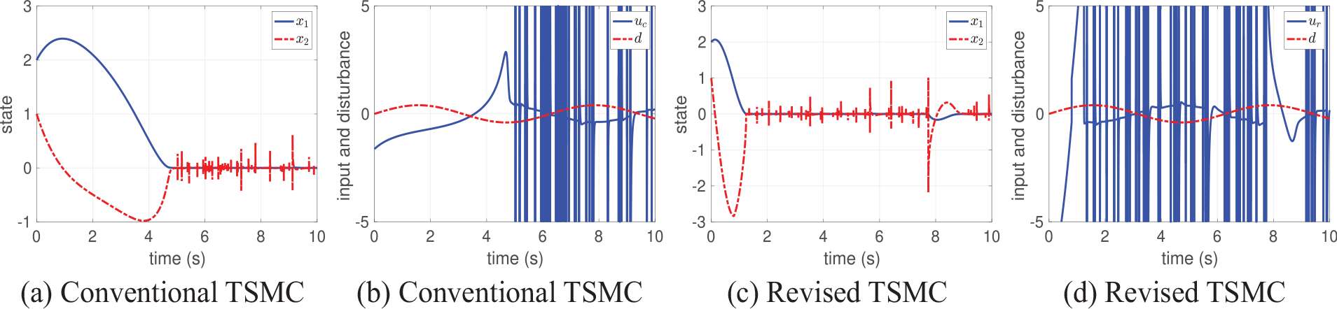
The simulation results are presented in Figure 5. TSMC satisfies the ISS condition by design and therefore, both conventional and revised TSMC are stable. The inherent singularity of TSMC causes unwanted spikes in the control signal for both cases. Nevertheless, the revised TSMC shows much faster convergence.

Figure 5.

Simulation of the conventional and revised TSMC for Example 5.

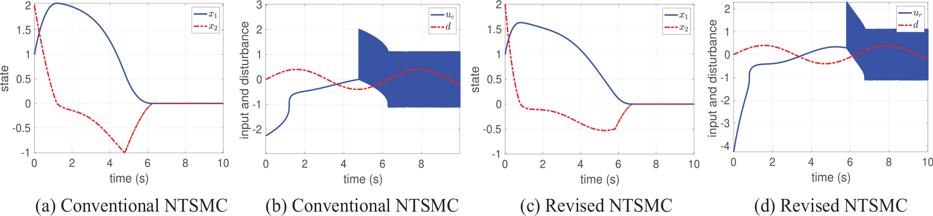
Example 6: Conventional versus revised NTSMC: Consider system (65) given in Example 5. The designed controller signal based on the conventional NTSMC, as in (21), is

u (x) = - sign (s) - x_{2}^{\frac{1}{3}},

(69)

s (t) = x_{1} + \frac{3}{5} x_{2}^{\frac{5}{3}} .

(70)

On the other hand, the designed revised NTSMC, as in (22), is

u (x) = - sign (s) - x_{2}^{\frac{1}{3}} - x_{2} .

(71)

The simulation results are presented in Figure 6. NTSMC satisfies the ISS condition by design and therefore, both conventional and revised NTSMC are stable. The figure shows that the revised NTSMC has smaller state peaks and therefore, a better transient behaviour.

Figure 6.

Simulation of the conventional and revised NTSMC for Example 6.

Conclusion

SMCs are widely used for their robustness against bounded matched uncertainties. In these controllers, the ISS condition should hold for stability. Global asymptotic stability of six Lyapunov-based SMCs were studied in this paper. We used a Lyapunov-based stability analysis for these controllers, which led to a new generation of SMCs with guaranteed global asymptotic stability and without the ISS condition. We conjecture it is possible to revise any Lyapunov-based SMC using the proposed method. The numerical examples illustrated the importance of revised controllers in which the revised SMCs were stable while the conventional ones were not in some cases. The study of additional aspects of revised SMCs such as performance, robustness, and ultimate bound requires more investigation.

Footnotes

Acknowledgements

The authors would like to thank members of ACSL (Advanced Control Systems Lab.) of University of Tehran for the fruitful discussion on the subject.

Declaration of conflicting interests

The author(s) declared no potential conflicts of interest with respect to the research, authorship, and/or publication of this article.

Funding

The author(s) received no financial support for the research, authorship, and/or publication of this article.

ORCID iDs

Mohammad Javad Yazdanpanah

Mohammad Reza Jahed-Motlagh

References

Asl

Hagh

Palm

(2017) Robust control by adaptive non-singular terminal sliding mode. Engineering Applications of Artificial Intelligence 59: 205–217.

Azar

Zhu

(eds) (2015) Advances and Applications in Sliding Mode Control Systems. Studies in Computational Intelligence, 576. Cham: Springer International Publishing.

Bartolini

Pisano

Punta

Usai

(2003) A survey of applications of second-order sliding mode control to mechanical systems. International Journal of Control 76(910): 875–892.

Bhat

Bernstein

(2000) Finite-time stability of continuous autonomous systems. SIAM Journal on Control and Optimization 38(3): 751–766.

Ding

(2017) Second-order sliding mode controller design subject to mismatched term. Automatica 77: 388–392.

Feng

Man

(2002) Non-singular terminal sliding mode control of rigid manipulators. Automatica 38(12): 2159–2167.

Fridman

Shtessel

Edwards

Yan

(2008) Higher-order sliding-mode observer for state estimation and input reconstruction in nonlinear systems. International Journal of Robust and Nonlinear Control: IFAC-Affiliated Journal 18(4–5): 399–412.

Han

Kao

Gao

(2017) Robust sliding mode control for uncertain discrete singular systems with timevarying delays and external disturbances. Automatica 75: 210–216.

Khalil

(2002) Nonlinear Systems. Upper Saddle River, NJ: Prentice hall.

10.

Laghrouche

Plestan

Glumineau

(2007) Higher order sliding mode control based on integral sliding mode. Automatica 43(3): 531–537.

11.

Levant

(2005) Homogeneity approach to high-order sliding mode design. Automatica 41(5): 823–830.

12.

, et al. (2014) Fault-tolerant control of Markovian jump stochastic systems via the augmented sliding mode observer approach. Automatica 50(7): 1825–1834.

13.

Spurgeon

(1999) Output feedback stabilization of MIMO non-linear systems via dynamic sliding mode. International Journal of Robust and Nonlinear Control: IFAC-Affiliated Journal 9(5): 275–305.

14.

Moreno

Osorio

(2012) Strict Lyapunov functions for the super-twisting algorithm. IEEE Transactions on Automatic Control 57(4): 1035–1040.

15.

Polyakov

Fridman

(2014) Stability notions and Lyapunov functions for sliding mode control systems. Journal of the Franklin Institute 351(4): 1831–1865.

16.

Shtessel

Moreno

Fridman

(2017) Twisting sliding mode control with adaptation: Lyapunov design, methodology and application. Automatica 75: 229–235.

17.

Sontag

(2008) Input to state stability: Basic concepts and results. Nonlinear and Optimal Control Theory. Berlin, Heidelberg: Springer, pp. 163–220.

18.

Utkin

Shi

(1996) DecemberIntegral sliding mode in systems operating under uncertainty conditions. In: Proceedings of 35th IEEE Conference on Decision and Control, Vol. 4, pp. 4591–4596. IEEE.

19.

Vidyasagar

(2002) Nonlinear Systems Analysis, Vol. 42. Siam.

20.

Yang

Yin

(2018) Descriptor observers design for markov jump systems with simultaneous sensor and actuator faults. IEEE Transactions on Automatic Control 64(8): 3370–3377.

21.

Yang

Yin

(2019) Reduced order sliding mode observer-based fault estimation for Markov jump systems. IEEE Transactions on Automatic Control 64(11): 4733–4740.

22.

Yang

Jiang

Yin

(2018) Fault-tolerant control of time-delay Markov jump systems with itô stochastic process and output disturbance based on sliding mode observer. IEEE Transactions on Industrial Informatics 14(12): 5299–5307.

23.

Long

(2015) Finite-time consensus for second-order multi-agent systems with disturbances by integral sliding mode. Automatica 54: 158–165.

24.

Zhihong

Paplinski

(1994) A robust MIMO terminal sliding mode control scheme for rigid robotic manipulators. IEEE Transactions on Automatic Control 39(12): 2464–2469.