






Abstract
This study analyzes with the technology of auto tuning using relay feedback test for non-square MIMO system through process modeling, identification, input-output pairing and control strategies. However, the control configuration selection based on conventional steady-state Relative Gain Array (RGA) matrix sometimes degrades the loop performance and it needs attention. This study also deals with the real challenges in time domain modeling and appropriate pairing of loops for non-linear chemical processes. The choice of input-output pairing for square system has been extended to non-linear chemical processes. This ensures the system’s stability by selecting an appropriate manipulated-controlled variable pairing in non-linear chemical processes and the same is also tested for benchmark of non-linear chemical processes. In this study, two types of non-square systems are considered: one is systems with excess input than output variables and the other is systems with excess output than input variables. Some benchmark non-linear chemical processes, such as processes with mild nonlinearity, moderate to high nonlinearity and highly nonlinearity, are also taken for this study. Three standard benchmark processes are used in analysis of nonlinear chemical processes, namely: (1) Continuous Stirred Tank Reactor (CSTR) process; (2) hydrogen-ion- concentration (pH) process and (3) distillation column and this procedure is illustrated via simulation of 3-by-2 and 2-by-3 non-linear chemical processes.
Keywords
Introduction
In a process having only one input variable used for controlling one output variable, the design of controller is simple. In most chemical and industrial processes the controller design is complex, as the system has multiple inputs and multiple outputs, making it multivariable in nature. Thus, with a multivariable process having equal number of input variables and output variables, such systems are termed as square systems because their transfer function matrices are square. Many benchmark square systems are given in the literature (Luyben, 1986). However, some of the multivariable systems have a number of input variables that are not equal to number of output variables. Such multivariable systems are termed as non-square systems. There are two types of non-square systems: systems that have fewer inputs than output variables will be referred to as under defined systems, while the systems with more input than output variables will be referred to as over defined systems. The under defined systems have a deficiency in input variables and over defined systems have an excess of input variables. Thus, non-square multivariable systems with n output variables and m input variables whose transfer function matrix will therefore be of dimension n x m. The system is under defined if m < n, and the system is over defined if m > n.
In the case of non-square systems, the most obvious problem with that after input-output pairing is there will be always a residual of unpaired input or output variables, depending on which of these are in excess. The innovation in this study, the nontrivial issue in non-square systems is addressed. Apart from these nontrivial issues, the other issue is which variable should be left redundant and which ones should take an active part in the control scheme.
The main issue in under defined Multi Input Multi Output (MIMO) system is that not all the outputs can be controlled since we do not have enough input variables. In the case of over defined MIMO system, we have an excess of input variables, and therefore we can actually achieve arbitrary control of the fewer output variables in more than one way. The limits of applicability of both under defined and over defined MIMO systems are very difficult to control.
Some of the multivariable processes are non-linear chemical processes exhibiting non-square MIMO systems. For example, mixing tank process (Arkun and Reeves, 1989) 2-by-3 system, shell control problem (Vlachos et al., 1999) 7-by-5 system, and so forth, are typical non-square multivariable process in industry. Three benchmark non-linear chemical processes are identified as non-square MIMO processes, namely, a mild non-linear Continuous Stirred Tank Reactor (CSTR) process (Khalid and Dawood, 2015) having two manipulated variables and three controlled variables; a Hydrogen-ion-concentration (pH) neutralization process (Henson and Seborg, 1994) having moderate to high non-linearity and highly non-linear distillation column (Marlin, 1986) having three manipulated variables and two controlled variables.
Astrom and Hagglund (1984) first proposed the relay feedback test for process control practitioners as a closed-loop tool for system identification and control. As the non-linear chemical processes are multivariable in nature, Shen and Yu (1994) proposed sequential method of identification for automatic control of multivariable systems. To synthesize a control system, singular value decomposition (SVD) framework for non-square linear systems was proposed by Lau et al. (1985). For non-square linear systems, block relative gain array, relative gain array are derived by Arkun and Reeves (1989) and Chang and Yu (1990). He et al. (2007) proposed equivalent transfer function method to non-square MIMO systems for Proportional Integral/Proportional Integral Derivative (PI/PID) decoupled controller design. The method has been applied to example with right half plane zero as given in the literature by Sarma and Chidambaram (2005). Further for two input two output system modelling and parameter estimation was proposed by Sujatha and Panda (2012). Sujatha and Panda (2013b) derived the novel method of interaction measure to select the proper input-output pairs. Mnasser and Bouani (2015) proposed the robust predictive controller for a class of multi-input–multi-output non-linear systems. Modeling and control of non-square systems using relay-feedback method were discussed by Kalpana et al. (2015). Saidi et al. (2019) studied the comparsion of internal model controller for non-square systems. In many of the above works, a dummy variable has been added to make the system as squared one for making the design to follow conventional way.
As the non-linear chemical processes are sensitive to plant parametric uncertainty, it is desired to design the robust feedback control system to utilize the technique that addresses all the plant variations up front; incorporates the information on desired output tolerance and mantaining the reasonable loop gain. Using the quantitative feedback theory, a compensator and prefilter may be designed to achieve a specified robust design which will be presented in future research work.
In general, all the literatures, the non-square systems are treated as square systems for control purpose either by discarding some inputs or by adding new outputs. Similarly, by eliminating some inputs can cause performance degradation and by appending new outputs can incur unnecessary cost. This focuses the motivation of research in these non-square systems. The contribution of this study is to bring the clear picture on how to model and control both the types of non-square MIMO systems.
The entire paper is organized as follows: Section 1 deals with the introduction. Section 2 discusses non-square MIMO systems and its types. Case studies on non-linear systems are discussed in Section 3. Section 4 highlights the proposed methodology and it includes algorithm and flow chart. Modeling, validation and parameter estimation of non-linear chemical processes are explained in Section 5. Control configuration selection based on conventional and proposed method for both the types of non-square MIMO systems are presented in Section 6. Closed loop studies and stability analysis are given in Sections 7 and 8, respectively. Conclusions are given in Section 9.
Non-square MIMO systems and its types
Block diagram of under defined non-square systems
Consider an open-loop under defined non-square MMO systems with n-1 inputs and n outputs. The system considered in this work has 2-inputs and 3-outputs. The general formulation of 3-by-2 MIMO system is shown in Figure 1. Figure 2 represents the block diagram of open-loop 3-by-2 nonsquare MIMO system. Here, m is the input variables, y is the output variables. The process transfer function matrix, G is expressed by equation (1).

General formulation of 3-by-2 nonsquare MIMO system.

Block diagram of open loop 3-by-2 nonsquare MIMO system.
The input and output variables are
The transfer function of Orgunnaike and Ray (OR) (1979) distillation column given by equation 2 represents the multiproduct plant distillation column for the separation of binary mixture of ethanol-water. The top compositions are controlled by manipulating the flow rates, pressure of the reflux and the reboiler stream. In this study, feed flow rate is considered as the disturbance. The input variables of the process are overhead reflux flow rate, side stream draw off rate and reboiler stream pressure. The output variables are overhead mole fraction of ethanol, side stream mole fraction of ethanol and the 19th tray temperature.
Consider the situation in which the binary distillation column used in this case has its sidestream draw-off rate set at a fixed amount that cannot be changed, and yet all three of its output variables – the overhead mole fraction of ethanol, the sidestream mole fraction of ethanol, and the Tray #19 temperature – are still being monitored, and are to be controlled. The benchmark underdefined non-square system considered here is Orgunnaike and Ray distillation column, given in equation (3)
where the input variables m1 and m2 are, respectively, the overhead reflux rate and the reboiler steam pressure. It is impossible to control all three output variables with only two input variables; however, the side stream mole fraction of ethanol is deemed the least important of the output variables, leaving two output variables to be controlled with the two input variables.
Upon deciding to leave the control of the side stream composition out of the control scheme, we may now rewrite the model as
along with the additional relation
From equation (4), the 3-by-2 underdefined non-square MIMO systems are treated as 2-by-2 square MIMO systems, as shown in Figure 3.

Modified block diagram of 3-by-2 nonsquare MIMO system.
Using Skogestad’s half rule (2003), elements in the transfer function matrix are approximated to First Order Plus Dead Time (FOPDT) model. Hence, the modified transfer function matrix of equation (4) is represented as
Block diagram of over defined non-square systems
Similarly, an over defined non-square MMO systems has n inputs and n-1 outputs. The system considered in this work has 3-inputs and 2-outputs. Figure 4 and Figure 5 represents the general block diagram and open loop transfer function of 2-by-3 MIMO system. Here, m is the input variables, y is the output variables and G is process transfer function matrix, expressed by equation (6)

General block diagram of 2-by-3 nonsquare MIMO system.

Open loop model of 2-by-3 MIMO system.
From the block diagram it is obvious that the non square is difficult to control as it is has an unequal number of inputs and output.
For the systems with 3 inputs and 2 outputs, that is, 2-by-3 MIMO system can be divided into three subsystems with all the possible combinations of 2-by-2 MIMO systems, whose block diagrams are represented in Figures 6, 7 and 8, respectively, with different combinations of inputs.

Block diagram of subsystem1.

Block diagram of subsystem2.

Block diagram of subsystem3.
Through pulse testing, the following transfer function model was obtained
This is a 2-by-3 MIMO system, and as such, we have a situation in which only two of the three candidate input variables will be used for control, while the third input variable will have to be set at a fixed value, and will therefore be redundant.
To determine which variable should be active and which should be redundant, we first obtain all the possible 2-by-2 MIMO subsystems; there are three such subsystems.
Case studies
In this research, work focuses on three benchmark non-linear chemical processes with various types of nonlinearity, starting from mild to highly non-linear systems.
The following case studies are done in this study, namely: (1) CSTR process–mildly nonlinear system; (2) pH neutralization process–moderate to high nonlinear system and (3) distillation column–highly non-linear system, and these problems are identified and the results on parametric identification and control are obtained using relay feedback test.
CSTR process
In the present case, a laboratory CSTR reactor system shown in Figure 9 is considered in which the reactants are sodium hydroxide (NaOH) and ethyl acetate (EtAc). The products due to alkaline hydrolysis of ester are sodium acetate and ethyl alcohol. This CSTR process has inlet flow rate (F) and cooling flow in jacket (Fj) as the manipulated variables. The controlled variables are concentration (CA), reactor absolute temperature (T) and cooling water temperature (Tj).

Representation of a CSTR system.
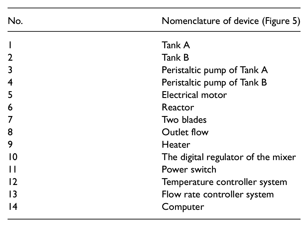
The CSTR process has two manipulated and three controlled variables and is categorized as 3-by-2 under defined non-square MIMO systems.
This process can be treated as square MIMO systems with ethyl acetate and hot water as manipulated variables and reaction temperature and ethyl acetate concentration as controlled variables. The process transfer function matrix of CSTR process is presented in equation (11)
pH process
Most of the physical pH processes exhibit nonlinear behaviour to some degree. The nonlinearities are of either mild or high type. The schematic of pH neutralization process is shown in Figure 10.

A schematic representation of pH neutralization process.
Referring to Bagher et al. (2011), the transfer function matrix of pH neutralization process is given in equation (12)
The pH neutralization process has three input variables such as flow-rates (Q) of acid, base and buffer; and two output variables as pH and level (h) of the tank. Hence, the process is defined as 2-by-3 over defined non-square MIMO system. The process is treated as square MIMO systems where pH2 and h2 are to be controlled variables using Q4 and Q6 as the manipulated variables with Q1 and Q3 held constant. The resulting process transfer function matrix is represented in the following equation (13)
Distillation column
The design of binary distillation process shown in Figure 11 was suggested by Weischedel and McAvoy (1981) is a highly nonlinear chemical process.

A schematic of a binary distillation tower.
The parameters (Table 1) of the distillation tower are listed below.
Operating variables of the binary distillation column.
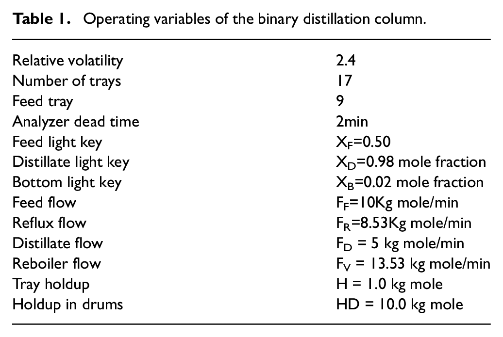
The potential manipulated variables of the distillation process are reflux (FR) and reboiler flow rate (FV), whereas distillate (XD) and bottom composition (XB) are the controlled variables here. The disturbance variable is the feed composition (XF).
The outputs are recorded by conducting experiment on each input variables. From the process reaction curve, the transfer functions are obtained for the distillation column is described by the following equation
This nonlinear system has three input variables and two output variables. Hence, the distillation column is defined as 2-by-3 over defined non-square systems.
The same system can be treated as square system whose transfer function matrix (equation 16) is described as
Proposed methodology
Algorithm
4.2. Flowchart
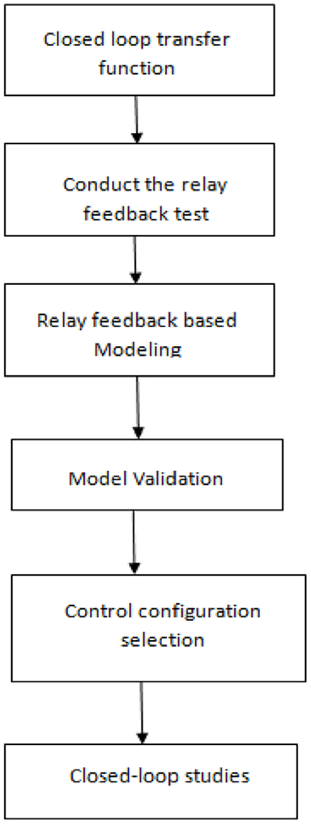
Modeling and validation for non-linear chemical processes using relay feedback test
As shown in Figure 12, consider n-by-n MIMO systems with decentralized PI controller.

Block diagram of n-by-n multivariable systems with decentralized PI controller.
The general modified transfer function of non-square MIMO systems represented as 2-by-2 square MIMO systems is described by
In auto tuning procedure the initial relationship between y and m is simply as
where the subscript OL denotes the open-loop. When the loop is closed sequentially, the closed-loop relationship between y and m becomes complicated. Therefore, it is considered that all the individual transfer functions of 2-by-2 MIMO systems are of FOPDT types.
In this case, the off-diagonal closed-loop transfer function can be found as
The above Equations (19) and (20) give interaction measure in closed-loop sense and the MIMO auto tuning can be done by sequential tuning procedures. Consider a 2-by-2 MIMO system with a known pairing (y1- m1); (y2- m2) under decentralized control. Then, the sequential auto tuning approach has several advantages; firstly, it makes the problem simple. The reason is that the proposed approach treats the MIMO system as a sequence of SISO systems where the relay feedback system is proven to be useful and reliable. Secondly, it operates in an efficient manner and, thirdly, it is a more accurate approach in terms of identification.
The procedure for MIMO auto tuning is described as follows.
As shown in Figure 13(a), initially a relay is placed between y1 and m1, while loop 1 is on manual mode. Following the relay feedback test, a controller for loop 1 can be designed from the ultimate gain and ultimate frequency.

(a) Step 1 of sequential method of tuning for 2-by-2 multivariable system.
The next step, as shown in Figure 13(b), is to perform relay feedback test between y3 and m2, while loop 1 is on auto mode. A controller can be designed for loop 2 following the relay feedback test.
As shown in Figure 13(c), once the controller on loop 2 is set on auto mode, another relay feedback test is formed between y1 and m1. In general, a new set of tuning constants is found for the controller in loop 1 and this procedure is repeated until the controller parameter converges. Typically, the controller parameter converges in 3–4 relay feedback tests in the case of 2-by-2 MIMO systems.
Modeling of non-square MIMO systems using ideal relay feedback test
The procedure for obtaining mathematical model of MIMO systems are explained in detail by Sujatha and Panda (2012). The ideal relay response for equation (14) is assumed to be formed by n-number of small step changes. At the first instant, (after synchronizing input with output by time shift) the response can be described as
Where, the term y1(t-1) is one step ahead prediction of y1.
At the second instant, the time is reset to zero at the initial point. The step response (relay output) can be given by: (i.e. introducing a time shift by D amount in equation (21))
where
Equation (22) can be simplified as follows
The relay response at the third interval lags by an amount D21+Pu/2 and D22+Pu/2 from an input of I and II parts: Thus, the above equation can be given as
Equation (24) can be easily simplified as
It can be seen from the above equation that the terms in the RHS (i.e. yn = y1+y2+y3+…… is the sum of the step responses at t1, t2, t3….) are slowly forming a series. As the time tends to infinity the response becomes stabilized and it can be described as yn = y1+y2+y3+……. In general, the ultimate properties are found out in 3–4 iterations, which are enough to get converged properties of ultimate parameters (Ku and Pu)
Let
In equation (20), RHS has four parts
The RHS of the above series becomes
First part = [1-2+2-2+…. upto
Similar way, Third part = 1
Second part =
This second part can be substituted into following series
Second part =
Similar way, Fourth part =
Thus, the generalized analytical expressions for equation (20) using ideal relay feedback test for 2-by-2 MIMO system is given by
The term yn(t-1) in Equation (27) is one step ahead prediction of yn.
Similarly, the generalized analytical expressions for equation (19) using ideal relay feedback test for 2-by-2 MIMO system is given by
The term yn(t-1) in equation (28) is one step ahead prediction of yn.
Model validation for 2-By-2 MIMO systems
The analytical expressions (developed in equations (21) and (22)) provide the mathematical models for undesirable relay responses of MIMO system. These theoretical equations are validated for non-square systems having 2-by-2 MIMO structure using ideal relay feedback tests for the period from t=0 to t=PU/2, respectively.
From Figure 14, it can be seen that the validation of the derived mathematical models where theoretical response of 3-by-2 non-square MIMO systems matches exactly with experimental one for ideal relay feedback tests.

Validation of analytical expression (dashed) of 3-by-2 non-square MIMO systems with experimental ideal relay response (solid) for OR process.
Similarly, the model validation of all the subsystems of the example taken for over defined non-square MIMO systems are shown in Figures 15, 16 and 17, respectively.

Validation of analytical response of subsystem 1 of 3-by-2 over defined non-square MIMO systems.

Model validation response of subsystem 2.

Model validation response of subsystem 3.
From the above figures, it is clear that undesired relay responses obtained after simulating the benchmark under defined and over defined non-square MIMO systems are compared with its original ideal relay responses and it is validated.
The model validation is done for all the nonlinear benchmark chemical processes described in Section 3 by simulation using MATLAB.
Figure 18 shows the model validation curve for CSTR chemical process and it is observed that the theoretical response curve matches exactly with the simulated response curve.

Model validation of analytical expression (dashed) of nonlinear chemical process with experimental ideal relay response (solid) for CSTR process.
The model validation is conducted for the pH process and it is found that the theoretical curve is approximately following the simulated curve as depicted in Figure 19.

Validated response of pH process.
For the distillation column, the ideal relay response for both theoretical and experimental are validated and it is represented in Figure 20 depicting the model validation.

Model validation for distillation column.
From these responses, it is clear that the experimental ideal response matches the theoretical ideal relay response for the nonlinear chemical processes.
Identification of parameters of 2-By-2 MIMO systems
The parameters of nonlinear chemical processes are estimated as given in Sujatha et al. (2013a) by formulating and applying the following boundary conditions to equations (27) and (28).
where m represents the model, a represents amplitude and D* for apparent dead time.
Applying the boundary conditions from equations (29) to (32) in the generalized analytical expression for 2-by-2 MIMO process, one can obtain the unknown parameters
The steps involved to estimate the parameters of 2-by-2 MIMO system:
From the undesired relay response, find out the dead times D21 and D12 from initial part of response.
Similarly, from the desired relay response obtain the dead times D22 and D11 from initial part of response.
Solve the equations simultaneously by applying the boundary conditions, to find unknown parameters k21, τ21, k22, τ22, k12, τ12, k11, τ11 of 2-by-2 MIMO system.
Tables 2 and 3 show the comparison between the true and estimated parameters of non-square MIMO systems and also error between these two values.
Comparison of true and estimated parameters of under defined non-square MIMO systems.
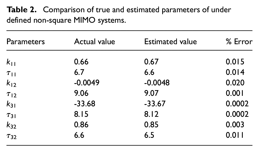
Comparison of true and estimated parameters of over defined non-square MIMO systems.
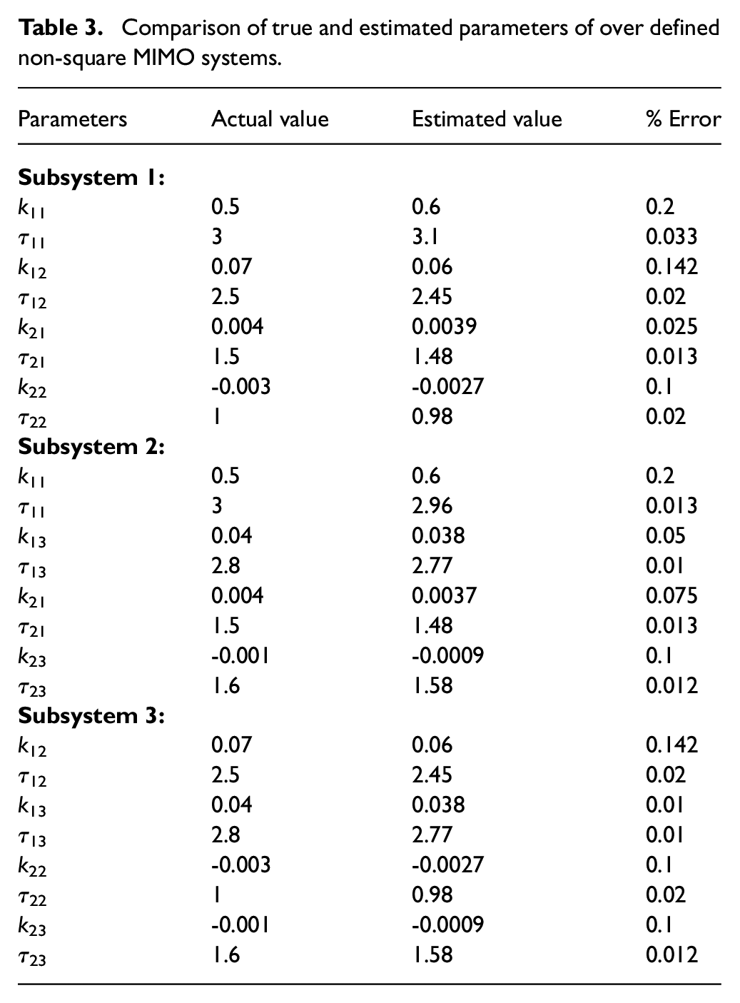
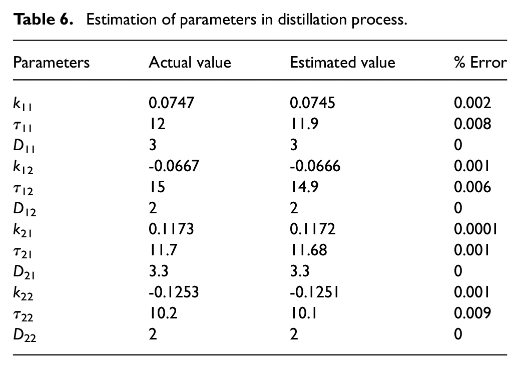
Tables 4, 5 and 6 show the error between the true and estimated parameters of benchmark nonlinear chemical processes. This method of parameter estimation is efficient in identifying the parameters of non-square MIMO processes.
CSTR process parameter estimation.
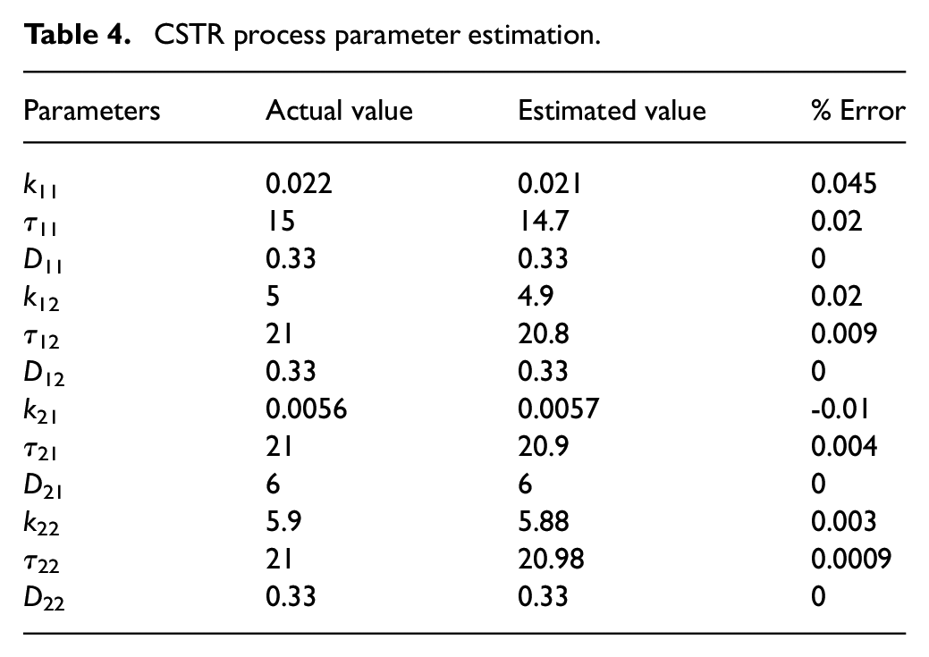
Parameter estimation of pH process.
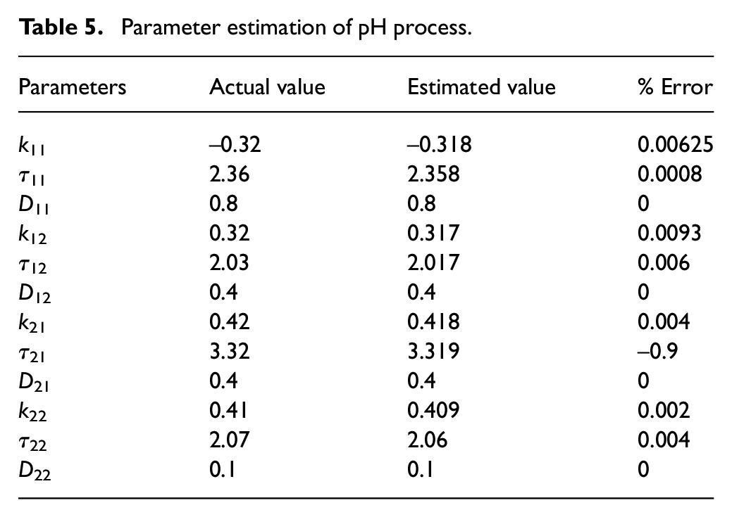
Estimation of parameters in distillation process.
Data from undesired closed-loop containing information on interactions (loop) are used for identifying the unknown process parameters. Parameter estimation algorithms using ultimate properties and land mark points are formulated to identify model parameters. The method is efficient for identifying MIMO process parameters.
Control configuration selection of non-square systems
Conventional method of loop pairing for under defined non-square MIMO systems
The modified (square) subsystem’s steady-state gain matrix is obtained as
The recommended input/ output pairing scheme is:
y1– m1; overhead reflux to control overhead composition
y3– m2; reboiler steam pressure to control Tray #19 temperature
The strategy is to choose a square subsystem by dropping off the excess number of output variables on the basis of economic importance; the subsequent analysis is the same as for square systems.
Proposed method of loop pairing under defined system
The under defined systems have two inputs (m1 and m2) and three outputs (y1, y2 and y3) and are squared by leaving y2 and expressed as 2x2 square MIMO systems. The square system that have two inputs (m1 and m2) and three outputs (y1 and y3) are considered. The proposed method of loop pairing is done by comparing the area under undesired responses for both diagonal and off-diagonal pairing, as given by Sujatha et al. (2013b). The pair that offers minimum area is chosen as a judicious loop pairing.
(y1-m1); (y3-m2) pairing
Figure 21 and Figure 22 show the closed loop undesired responses for diagonal pairing and the area under the curve is obtained in Table 7.
(y1-m2); (y3-m1) pairing

Closed loop undesired response for diagonal pairing of OR column, (y3/m1).

Closed loop undesired response for diagonal pairing of OR column, (y1/m2).
Comparison of areas under the disturbance/ load responses for OR column.
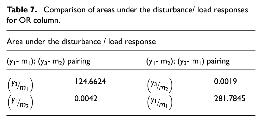
The closed loop response for off diagonal pairing is shown in Figure 23 and Figure 24 and its corresponding area is tabulated in Table 7.

Closed loop undesired response for off diagonal pairing of OR column, (y3/m1).

Closed loop undesired response for off diagonal pairing of OR column, (y1/m2).
From Table 7, it is clear that the desirable pairing for OR column is (y1− m1); (y3− m2) pairing.
Conventional method of loop pairing for over defined non-square MIMO systems
RGA: In this case, we have an excess of input variables, and therefore we can actually achieve arbitrary control of the fewer output variables in more than one way. The strategy for loop pairing is:
First determine, from the given process model, all the
Obtain the RGAs for each of these square subsystems.
Examine these RGAs and pick the best subsystem on the basis of the overall character of its RGA (in terms of how close it is to the ideal RGA).
Having thus determined the best subsystem, use its RGA to determine which input variable within this subsystem to pair with which output variable.
Next, RGA for each subsystem are obtained and the results are as follows.
For subsystem 1
For subsystem 2
For subsystem 3
Based on inspection of these three RGAs, it appears that Subsystem 1 will offer us the best possible control, because its RGA is the closest to the ideal situation; it is somewhat better than Subsystem 2, and far superior to Subsystem 3.
Having thus decided on Subsystem 1, the implication is that the input variables m1 and m2 are to be used for control and m3 is to be redundant. The final task is to pair the variables of this subsystem, an easy exercise. The best possible loop pairing within this subsystem is y1– m1 and y2– m2.
This example has shown that for under defined systems, the strategy is to choose a square subsystem by dropping off the excess number of output variables on the basis of economic importance; the subsequent analysis is the same as for square systems.
Proposed method of loop pairing – over defined system
The pairing for over defined systems having three inputs and two outputs can be treated as three subsystems having two inputs and two outputs and the method used for pairing of the square system is extended.
Case 1: (y1-m1); (y3-m2) pairing
Subsystem 1 closed loop responses are plotted in Figures 25 and 26 and its area is given in Table 8.

Closed loop undesired response for diagonal pairing (y2/m1).

Closed loop undesired response for diagonal pairing (y1/m2).
Comparison of areas under the load responses for subsystem1.
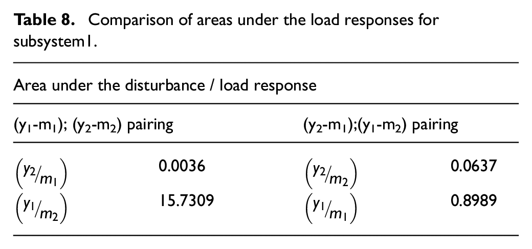
The undesired responses for off diagonal pairing are obtained in Figures 27 and 28 and its area is also given in Table 8.

Closed loop undesired response for off diagonal pairing (y2/m2).

Closed loop undesired response for off diagonal pairing (y1/m1).
Hence, desirable pairing for the subsystem 1 is (y2-m1); (y1-m2).
Case 1: (y1–m1); (y2-m3) pairing
For the diagonal pairing, the closed loop undesired responses are obtained in Figure 29 and Figure 30, respectively.

Closed loop undesired response for diagonal pairing (y2/m1).

Closed loop undesired response for diagonal pairing (y1/m2).
The closed loop undesired responses for off diagonal pairing for subsystem 2 is obtained in Figure 31 and Figure 32.

Closed loop undesired response for off diagonal pairing (y2/m2).

Closed loop undesired response for off diagonal pairing (y1/m1).
From Table 9, is clear that minimum area is obtained only for (y1-m3); (y2-m1) pairing. Hence, desirable pairing for the subsystem 2 is (y1-m3); (y2-m1).
Comparison of areas under the load responses for subsystem 2.
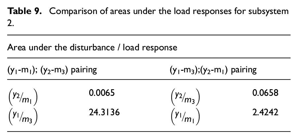
Similarly, the same procedure can be extended for subsystem 3. From subsystem 1 and 2, it is clear that for this particular system, the recommended input-output pairing is (y1-m3); (y2-m1).
Conventional method of loop pairing for non-linear chemical process
From Table 10, it is clear that from RGA matrix for all the benchmark process, the desirable input-output pair is (y1-m1); (y2-m2).
Conventional loop pairing method- relative gain array.

Proposed loop pairing for the non-linear chemical processes
The judicious choice of loop pairing is based on comparing the areas under the closed loop undesired responses for all combinations of input-output pairing. The pair that offers minimum area is chosen as a judicious choice of loop pairing.
Loop pairing of CSTR process
The loop pairing in CSTR process is obtained by assuming diagonal pairing and off diagonal pairing, the closed loop response are obtained and shown in Figures 33, 34, 35 and 36, respectively. The area under the closed loop undesired responses are calculated and its values are tabulated in Table 11 for comparison. The correct pairing is chosen based on the minimum area obtained after comparison.

Closed loop undesired response for diagonal pairing (y2/m1).
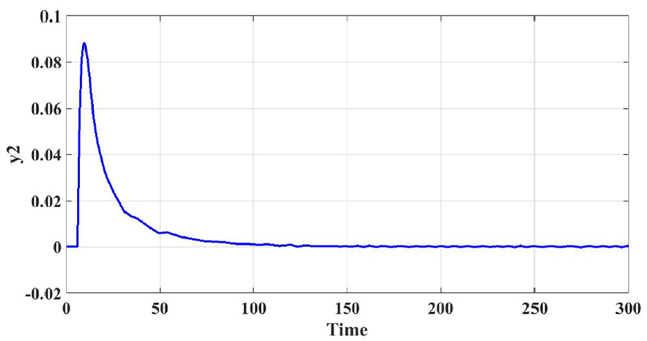
Closed loop undesired response for diagonal pairing (y1/m2).

Closed loop undesired response for off diagonal pairing (y2/m2).

Closed loop undesired response for off diagonal pairing (y1/m1).
Proposed loop pairing – Comparison of areas under the load responses.

Figure 33 represents the closed loop undesired response, y2 of CSTR process by assuming the diagonal pairing when there is change in input m1 while m2=0.
For CSTR process, the closed-loop undesired response, y1 when there is change in m2 for diagonal pairing of CSTR process is represented in Figure 34.
Figure 35 shows that for CSTR process, the closed loop undesired response y2 for the change in m2 by assuming off-diagonal pairing.
The closed loop undesired response y1 for the change in m1 for off diagonal pairing in CSTR process is represented in Figure 36.
Loop pairing of pH process
For the pH process, closed loop undesired responses are obtained for both diagonal and off-diagonal pairing as shown in Figures 37, 38, 39 and 40. The areas obtained under these curves are given in Table 11 and the same is compared to obtain the desired input-output pair based on minimum value.

Closed loop undesired response for diagonal pairing (y2/m1).

Closed loop undesired response for diagonal pairing (y1/m2).
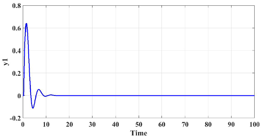
Closed loop undesired response for off diagonal pairing (y2/m2).

Closed loop undesired response for off diagonal pairing (y1/m1).
Figure 37 represents the closed loop undesired response y2 for the change in m1 for diagonal pairing of pH process.
For diagonal pairing in pH process, closed loop undesired response y1 for change in m2 is shown in Figure 38.
For the pH process, the closed loop undesired response y2 for change in m2 is represented in Figure 39 for off-diagonal pairing.
For off diagonal pairing in pH process, Figure 40 represents the closed-loop undesired response y1 for the change in m1.
Loop pairing of distillation column
Similar to CSTR and pH process, the pairing for distillation column are also carried out to choose the correct input-output pairing.
Closed loop undesired response for diagonal pairing of distillation column is represented in Figure 41.

Closed loop undesired response for diagonal pairing (y2/m1).
Figure 42 shows that closed loop response of distillation column for diagonal pairing.
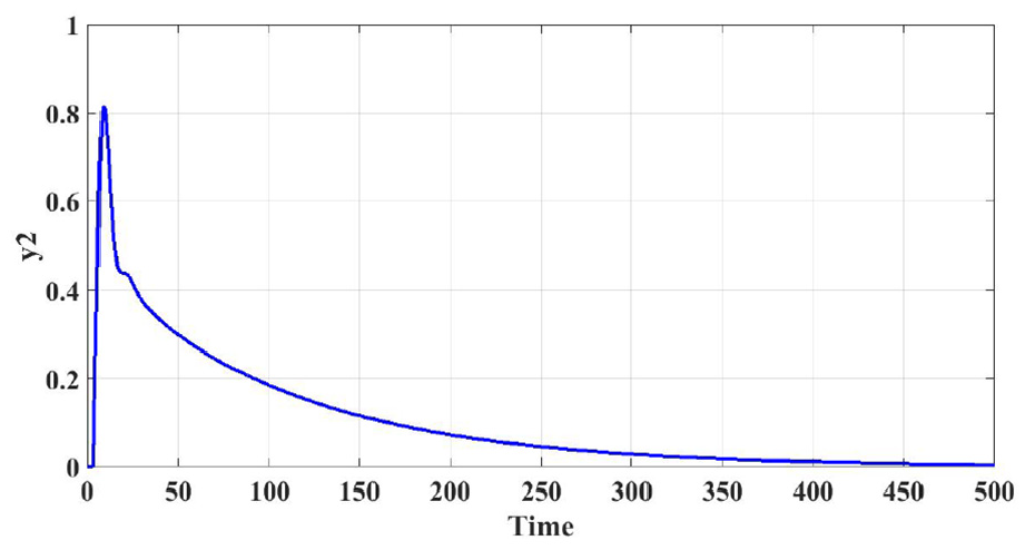
Closed loop undesired response for diagonal pairing (y1/m2).
For the distillation column, closed loop undesired response y2 for the change in m2 for off diagonal pairing is shown in Figure 43.

Closed loop undesired response for off diagonal pairing (y2/m2).
Figure 44 represents that the closed loop undesired response y1 for off diagonal pairing of distillation column

Closed loop undesired response for off diagonal pairing (y1/m1).
Similarly, Figures 41, 42 and Figures 43, 44 represent undesired responses for distillation column and its area is given in Table 11.
From Table 11, for all benchmark nonlinear chemical processes, it is clear that the minimum area is obtained only for (y1-m1); (y2-m2) pairing. Hence, desirable pairing for all these processes is
Closed loop controller tuning Internal Model Control-Proportional Integral Derivative (IMC-PID) laurent tuning rule
IMC-PI controller parameters are derived by equating the closed loop response to desired closed-loop response involving user defined tuning parameter, λ. Thus, the IMC-PI controller parameter by Panda (2009) for FOPDT processes are computed using the following expressions
Closed loop response of under-defined non-square MIMO system
The parameters of multi-loop controllers using IMC for SISO system has been extended to MIMO processes are listed in the following Table 12.
Controller parameters for under defined non-square MIMO system.
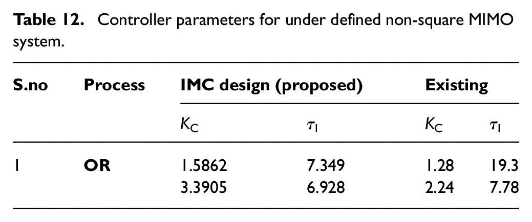
The simulation results given in Figure 45 shows that IMC design provides better performance.

Set response of under defined non-square MIMO systems.
Thus, the ISE values are compared for proposed and existing method for the under defined systems are tabulated in Table 13.
Comparison of ISE values for proposed and existing method.

Closed loop response of over defined non-square MIMO system
The controller parameters of subsystem 1, subsystem 2 and subsystem 3 are listed in Table 14.
Controller parameters of over defined non-square MIMO systems.

The closed-loop step responses for subsystem 1 and subsystem 2 of overdefined nonsquare MIMO systems are shown in Figures 46 and 47, better performance can be obtained by designing controllers using IMC. Similarly, the closed loop step responses for subsystem 3 can also be obtained.

Set response of subsystem1 of overdefined nonsquare MIMO systems.

Set response of subsystem 2 of overdefined nonsquare MIMO system.
Table 15 represents the comparison of ISE values for over defined MIMO systems.
ISE values for over defined systems.

Closed loop response of nonlinear chemical process
Table 16 represents the controller parameters for the nonlinear chemical processes
Controller parameters of over defined non-square MIMO systems.

The closed loop responses for these non-linear chemical processes are shown in Figures 48, 49 and 50, respectively.

Closed loop response of CSTR process for set point tracking.

pH process and its closed loop response.

closed loop response of distillation column.
ISE values for nonlinear chemical processes are tabulated in Table 17.
ISE values for nonlinear chemical processes.

Stability analysis of non-square systems
The characteristic equation of any system, closed loop or open loop, is the equation that you get when you take the denominator of the transfer function describing the system and set it equal to zero. The resulting Nth– order polynomial equation in s has N roots, and these dictate the stability, damping and speed of response of the system.
For closed loop systems by Luyben (1996), the denominator of the transfer functions in the closed loop servo and load transfer function matrices gives the closed-loop characteristic equation. The denominator is to be
This is the most important equation in multivariable control. It applies for any type of controller, diagonal (multi loop SISO) or full multivariable controller. If any of the roots of this equation are in the right half of the s plane, the system is closed loop unstable.
The closed loop characteristic equation for a 2x2 process with a diagonal feedback controller
The closed loop characteristic equation depends on the tuning of both feedback controllers.
Thus, the stability analysis of non-square MIMO systems are listed in Table 18. It is observed that the system is stable.
Stability analysis of non-square MIMO systems.

Conclusion
In this study, two types of non-square systems namely, underdefined and overdefined systems are modelled and controlled. The estimated parameters are obtained using the landmark points from the model. The control configuration selection has been done by capturing and comparing the area under the closed loop undesired responses for both diagonal and off-diagonal pairing. The pairing is decided based on area comparison, which gives the minimum area under the curve. The input-output pairing based on the proposed methods is carried out for both under defined and over defined non-square MIMO systems. Closed loop studies also carried out using IMC-based PI controller. The proposed method of modeling and control can also be extended to overdefined non-square MIMO systems with non minimum phase.
Footnotes
Declaration of conflicting interests
The author(s) declared no potential conflicts of interest with respect to the research, authorship, and/or publication of this article.
Funding
The author(s) received no financial support for the research, authorship, and/or publication of this article.
