Extended conjugate gradient squared and conjugate residual squared methods for solving the generalized coupled Sylvester tensor equations

Abstract

In this paper, two attractive iterative methods – conjugate gradient squared (CGS) and conjugate residual squared (CRS) – are extended to solve the generalized coupled Sylvester tensor equations $\sum_{j = 1}^{n} X_{j} \times_{1} A_{ij 1} \times_{2} A_{ij 2} . . . \times_{d} A_{ijd} = C_{i}, i = 1, 2, . . ., n$ . The proposed methods use tensor computations with no maricizations involved. Also, some properties of the new methods are presented. Finally, several numerical examples are given to compare the efficiency and performance of the proposed methods with some existing algorithms.

Keywords

Tensor equations CGS CRS iterative method

Introduction

Throughout this paper, tensors are written in calligraphic font, for example, $A$ . Let $d$ be a positive integer, an order $d$ tensor $A = (a_{i_{1} i_{2} . . . i_{d}}) (1 \leq i_{j} \leq n_{j}, j = 1, 2, . . ., d)$ is a multidimensional array with $N (N = n_{1} n_{2} . . . n_{d})$ entries (Kolda, 2006; Kolda and Bader, 2009). Each entry of $A$ is denoted by $a_{i_{1} i_{2} . . . i_{d}}$ . $O$ with all entries zero denotes the zero tensor. With this definition of tensor, matrices are tensors of order two where signified by capital letters, for example, $A$ . As usual, $C$ denotes the complex number field.

Recently, general tensor equations have attracted a lot of attentions (Beik et al., 2015, 2016; Li et al., 2010; Shi et al., 2013; Sun et al., 2016). In this paper, we are concerned with the generalized coupled Sylvester tensor equations

\sum_{j = 1}^{n} X_{j} \times_{1} A_{ij 1} \times_{2} A_{ij 2} . . . \times_{d} A_{ijd} = C_{i}, i = 1, 2, . . ., n,

(1)

where the matrices $A_{ijl} \in C^{n_{ijl} \times n_{ijl}}$ $(i, j = 1, 2, . . ., n$ and $l = 1, 2, . . ., d)$ , the tensors $C_{i} \in C^{n_{i 1} \times . . . \times n_{id}} (i = 1, 2, . . ., n)$ are known and tensors $X_{j} \in C^{n_{j 1} \times . . . \times n_{jd}} (j = 1, 2, . . ., n)$ are unknown and the definition of $j$ -mode product $\times_{j} (j = 1, 2, . ., n)$ is as the following definition.

Definition 1: (Kolda, 2006). The operators $\times_{k} (k = 1, 2, . . ., d)$ represent the $k$ -mode product of a tensor $X$ with a matrix $A \in C^{m \times n_{k}}$ defined as follows

(X \times_{k} A)_{i_{1} i_{2} . . . i_{k - 1} j i_{k + 1} . . . i_{d}} = \sum_{i_{k} = 1}^{n_{k}} x_{i_{1} i_{2} . . . i_{k - 1} i_{k} i_{k + 1} . . . i_{d}} a_{j i_{k}}

Definition 2: (Sun et al., 2016) For a tensor $A = (a_{i_{1} . . . i_{N} j_{1} . . . j_{M}}) \in C^{I_{1} \times . . . \times I_{N} \times J_{1} \times . . . \times J_{M}}$ , let $B = (b_{i_{1} . . . i_{M} j_{1} . . . j_{N}}) \in C^{J_{1} \times . . . \times J_{M} \times I_{1} \times . . . \times I_{N}}$ be the conjugate transpose of $A$ , where $b_{i_{1} . . . i_{M} j_{1} . . . j_{N}} = {\bar{a}}_{j_{1} . . . j_{M} i_{1} . . . i_{N}}$ . The tensor $B$ is denoted by $B^{*}$ . When $b_{i_{1} . . . i_{M} j_{1} . . . j_{N}} = a_{j_{1} . . . j_{M} i_{1} . . . i_{N}}$ , $B$ is called the transpose of $A$ , denoted by $A^{T}$ .

Definition 3: (Brazell et al., 2013) Let $N, M$ be positive integers. The inner product of two tensors $X, Y \in C^{I_{1} \times . . . \times I_{N} \times J_{1} \times . . . \times J_{M}}$ is defined by

$< X, Y > = \sum_{j_{M} = 1}^{J_{M}} . . . \sum_{j_{1} = 1}^{J_{1}} \sum_{i_{N} = 1}^{I_{N}} . . . \sum_{i_{1} = 1}^{I_{1}} x_{i_{1} . . . i_{N} j_{1} . . . j_{M}} {\bar{y}}_{j_{1} . . . j_{M} i_{1} . . . i_{N}},$

so the tensor norm that generated by this inner product is

$‖ X ‖ = \sqrt{< X, X >} = \sqrt{\sum_{j_{M} = 1}^{J_{M}} . . . \sum_{j_{1} = 1}^{J_{1}} \sum_{i_{N} = 1}^{I_{N}} . . . \sum_{i_{1} = 1}^{I_{1}} | x_{i_{1} . . . i_{N} j_{1} . . . j_{M}} |^{2}},$

which is the tensor Frobenius norm. We say that $X, Y$ are orthogonal if $< X, Y > = 0 .$

We define a new inner product that is needed in the continuing.

Definition 4: Let $(X, Y), (W, S) \in C^{n_{1} \times n_{2} \times . . . \times n_{d}} \times C^{n_{1} \times n_{2} \times . . . \times n_{d}}$ . Then

< < (X, Y), (W, S) > > = < X, W > + < Y, S > .

It is easy to show that $< < ., . > >$ is an inner product on linear space $C^{n_{1} \times n_{2} \times . . . \times n_{d}} \times C^{n_{1} \times n_{2} \times . . . \times n_{d}}$ and its associated norm is indicated by $| | . | |_{*}$ and is as $| | (X, Y) | |_{*} = \sqrt{| | X {| |}^{2} + | | Y {| |}^{2}} .$

For ease of notations and calculation, the linear equation system (1) can be defined as an operator form. To this end, we have the following definition.

Definition 5: Let $H_{j}, j = 1, 2, . . ., n$ be the linear space $C^{n_{j 1} \times . . . \times n_{jd}}, j = 1, 2, . . ., n .$ Then

\begin{matrix} L : H_{1} \times H_{2} \times . . . \times H_{n} \to H_{1} \times H_{2} \times . . . \times H_{n} \\ L (X_{1}, X_{2}, . . ., X_{n}) = (\begin{matrix} \sum_{j = 1}^{n} X_{j} \times_{1} A_{1 j 1} \times_{2} A_{1 j 2} . . . \times_{d} A_{1 jd} \\ \sum_{j = 1}^{n} X_{j} \times_{1} A_{2 j 1} \times_{2} A_{2 j 2} . . . \times_{d} A_{2 jd} \\ . . . \\ \sum_{j = 1}^{n} X_{j} \times_{1} A_{nj 1} \times_{2} A_{nj 2} . . . \times_{d} A_{njd} \end{matrix}) \end{matrix}

According to Definition 5, linear system (1) can be rewritten as

L (X_{1}, X_{2}, . . ., X_{n}) = C,

(2)

where $C = {({C_{1}}^{T}, {C_{2}}^{T}, . . ., {C_{n}}^{T})}^{T}$ .

When $X_{j}, j = 1, 2, . . ., n$ are an order 2 tensors, (1) reduces to

\sum_{j = 1}^{n} A_{ij 1} X_{j} A_{ij 2}^{*} = C_{i}, i = 1, 2, . . ., n,

which is the generalized coupled Sylvester matrix equations. Thus, (1) is called the generalized coupled Sylvester tensor equations. Generalized (coupled) Sylvester matrix equations have a wide range applications in system and control theory and the generalized eigenvalue problems (Ding and Chen, 2005a, 2005b; Golub et al., 1978; Kagström and Westin, 1989).

Several kinds of tensor equations (1) are as follows

X \times_{1} A_{1} + X \times_{2} A_{2} + . . . + X \times_{d} A_{d} = C,

(3)

X \times_{1} A_{1} \times_{2} A_{2} . . . \times_{d} A_{d} = C,

(4)

X \times_{1} A_{1} \times_{2} A_{2} . . . \times_{d} A_{d} + Y \times_{1} B_{1} \times_{2} B_{2} . . . \times_{d} B_{d} = C,

(5)

{\begin{matrix} X \times_{1} A_{1} \times_{2} A_{2} . . . \times_{d} A_{d} = C_{1}, \\ X \times_{1} B_{1} \times_{2} B_{2} . . . \times_{d} B_{d} = C_{2}, \end{matrix}

(6)

{\begin{matrix} X \times_{1} A_{1} \times_{2} A_{2} . . . \times_{d} A_{d} + Y \times_{1} B_{1} \times_{2} B_{2} . . . \times_{d} B_{d} = C_{1}, \\ X \times_{1} C_{1} \times_{2} C_{2} . . . \times_{d} C_{d} + Y \times_{1} D_{1} \times_{2} D_{2} . . . \times_{d} D_{d} = C_{2} . \end{matrix}

(7)

The tensor equation (3) often arises from the finite element, finite difference or spectral methods (Bai et al., 2003; Grasedyck, 2004; Li et al., 2009). Several methods are proposed for solving this equation. For example Chen and Lu (2012, 2013) have proposed the GMRES, CG and MCG-based on tensor form, respectively. Beik et al. (2016) also presented a conjugate gradient and a nested conjugate gradient algorithms with the tensor form by the Arnoldi process and the full orthogonalization method.

Definition 6: The tensor equations (1) are said to be consistent if there exist ${\tilde{X}}_{j}, j = 1, 2, . . ., n$ satisfying in $(1)$ , ${\tilde{X}}_{j}, j = 1, 2, . . ., n$ are said to be solution of (1).

To the best our knowledge, so far less iterative method has been applied to solve equation (1). These issues motivated the authors to present extended conjugate gradient squared and extended conjugate residual squared (CRS) algorithms to solve (1). These methods are based on tensor form and use tensor computations with no maricizations involved. As we know, the common conjugate gradient squared (CGS) and conjugate residual squared methods are two types of the most important and useful algorithms to compute the solution of non-Hermitian linear system

Ax = b, A \in C^{n \times n}, x \in C^{n} .

(8)

The remainder of this paper is organized as follows. In Section 2, we first review the common CGS and CRS algorithms for solving (8) and then extended CGS and CRS methods are obtained according to tensor form to solve (1). In Section 3, we present comparison results. Finally, some concluding remarks and acnowledgements are given in Section 4.

Extended CGS and CRS methods for solving (1)

In this section, first we present a short introduction to the common CGS and CRS methods to solve (8) and then extended CGS and extended CRS (called ECGS and ECRS, respectively) algorithms are presented for solving (1).

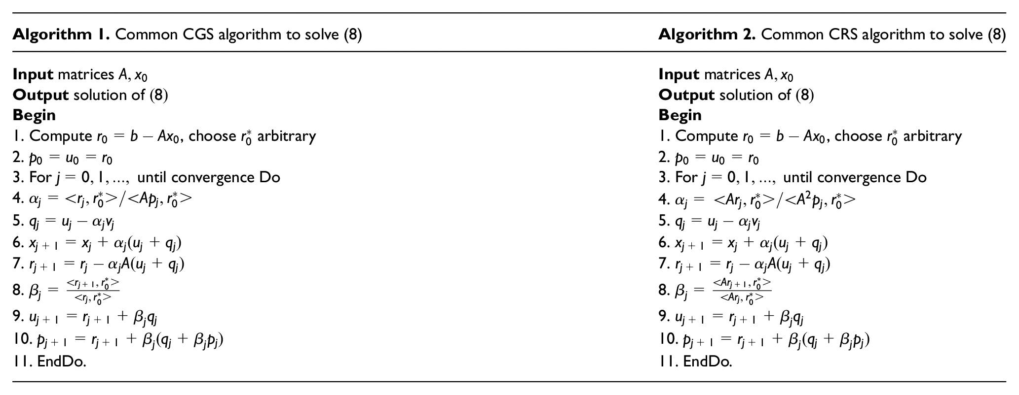
Two types of the iterative methods for solving large sparse non-Hermitian linear systems of equations are the bi-conjugate gradient (Bi-CG) and bi-conjugate residual (Bi-CR) methods that are based on the non-symmetric Lanczos procedure. For more details about Bi-CG and Bi-CR, one may refer to Saad (2003). The common conjugate gradient squared algorithm was developed by Sonneveld (1984), mainly to avoid using the transpose of $A$ in the Bi-CG and to gain faster convergence (the expected convergence rate is about twice that of the Bi-CG algorithm) for roughly the same computational cost. The common CGS algorithm for solving (8) is summarized in Algorithm 1. In exact arithmetic, the common CGS algorithm terminates with true solution after $j \leq n$ steps (see Sonneveld, 1984). By using Bi-CR and common CGS algorithms, the common CRS algorithm for solving (8) is shown in Algorithm 2.

Algorithm 1. Common CGS algorithm to solve (8)	Algorithm 2. Common CRS algorithm to solve (8)
Input matrices $A, x_{0}$	Input matrices $A, x_{0}$
Output solution of $(8)$	Output solution of $(8)$
Begin	Begin
1. Compute $r_{0} = b - A x_{0}$ , choose $r_{0}^{*}$ arbitrary	1. Compute $r_{0} = b - A x_{0}$ , choose $r_{0}^{*}$ arbitrary
2. $p_{0} = u_{0} = r_{0}$	2. $p_{0} = u_{0} = r_{0}$
3. For $j = 0, 1, . . .,$ until convergence Do	3. For $j = 0, 1, . . .,$ until convergence Do
4. $α_{j} = < r_{j}, r_{0}^{} > / < A p_{j}, r_{0}^{} >$	4. $α_{j} = < A r_{j}, r_{0}^{} > / < A^{2} p_{j}, r_{0}^{} >$
5. $q_{j} = u_{j} - α_{j} v_{j}$	5. $q_{j} = u_{j} - α_{j} v_{j}$
6. $x_{j + 1} = x_{j} + α_{j} (u_{j} + q_{j})$	6. $x_{j + 1} = x_{j} + α_{j} (u_{j} + q_{j})$
7. $r_{j + 1} = r_{j} - α_{j} A (u_{j} + q_{j})$	7. $r_{j + 1} = r_{j} - α_{j} A (u_{j} + q_{j})$
8. $β_{j} = \frac{< r_{j + 1}, r_{0}^{} >}{< r_{j}, r_{0}^{} >}$	8. $β_{j} = \frac{< A r_{j + 1}, r_{0}^{} >}{< A r_{j}, r_{0}^{} >}$
9. $u_{j + 1} = r_{j + 1} + β_{j} q_{j}$	9. $u_{j + 1} = r_{j + 1} + β_{j} q_{j}$
10. $p_{j + 1} = r_{j + 1} + β_{j} (q_{j} + β_{j} p_{j})$	10. $p_{j + 1} = r_{j + 1} + β_{j} (q_{j} + β_{j} p_{j})$
11. EndDo.	11. EndDo.

In the following, we provide the ECGS and ECRS algorithms for solving (1), but before this purpose it is necessary for us to review the properties of tensor $k$ -mode product used in this paper. The following theorems establish the associative law for the $k$ -mode product.

Theorem 1: (Kolda, 2006). If $A \in C^{n_{1} \times n_{2} \times . . . \times n_{d}}, M_{1}, M_{k} \in C^{m_{k} \times n_{k}}, M_{2} \in C^{p \times m_{k}}$ and $M_{j} \in C^{m_{j} \times n_{j}} (k \neq j)$ , then $(A \times_{k} M_{1}) \times_{k} M_{2} = A \times_{k} (M_{2} M_{1}), (A \times_{k} M_{k}) \times_{j} M_{j} = (A \times_{j} M_{j}) \times_{k} M_{k} .$

Theorem 2. (Kolda, 2006). If $A \in C^{p \times q}, X \in C^{n_{1} \times n_{2} \times . . . \times n_{k - 1} \times p \times n_{k + 1} \times . . . \times n_{d}}$ and $Y \in C^{n_{1} \times n_{2} \times . . . \times n_{k - 1} \times q \times n_{k + 1} \times . . . \times n_{d}}$ then

< X, Y \times_{k} A > = < X \times_{k} A^{*}, Y > .

The mode- $k$ matricization of a tensor $X \in C^{n_{1} \times n_{2} \times . . . \times n_{d}}$ is denoted by $X (k)$ and the mode- $k$ fibres are arranged to be the columns of the resulting matrix (Kolda and Bader, 2009). The operator “ $vec$ “ denotes the columns of a matrix or tensor to form a vector (Kolda and Bader, 2009). For a matrix $A = (a_{1}, a_{2}, . . ., a_{n}) = (a_{ij}) \in C^{m \times n}$ and a matrix $B$ , $A \otimes B = (a_{ij} B)$ is a Kronecker product and $vec (A) = (a_{1}^{T}, a_{2}^{T}, . . ., a_{n}^{T})^{T}$ , where $a_{i}, 1 \leq i \leq n$ is the $i$ -th column of $A$ and for a tensor $X \in C^{I_{1} \times I_{2} \times . . . \times I_{N}}$ , $X (1)$ is the mode-1 matricization of the tensor $X$ . By using the property of the Kronecker product, it can be shown that tensor equations (1) are equivalent to the following equations

\sum_{j = 1}^{n} G_{ij} vec (X_{j}) = vec (C_{i}), i = 1, 2, . . ., n,

where

G_{ij} = A_{ijd} \otimes . . . \otimes A_{ij 2} \otimes A_{ij 1}, i, j = 1, 2, . . ., n,

and ⊗ stands for Kronecker product.

By means of Kronecker product and vectorization operator, the general coupled tensor equations (1) can be transformed into the following linear system

\underset{A}{\underset{︸}{(\begin{matrix} G_{11} & G_{12} & . . . & G_{1 n} \\ G_{21} & G_{22} & . . . & G_{2 n} \\ . . . & . . . & . . . & . . . \\ G_{n 1} & G_{n 2} & . . . & G_{nn} \end{matrix})}} \underset{x}{\underset{︸}{(\begin{matrix} vec (X_{1}) \\ vec (X_{2}) \\ . . . \\ vec (X_{n}) \end{matrix})}} = \underset{b}{\underset{︸}{(\begin{matrix} vec (C_{1}) \\ vec (C_{2}) \\ . . . \\ vec (C_{n}) . \end{matrix})}}

(9)

The linear system (9) is consistent if and only if (1) is consistent. The size of (9) is very large even for small values of $n$ and thus the using of common CGS and CRS algorithms to solve (9) instead of solving corresponding tensor equations (1) will consume much more computer time and memory space when the dimension increases. In order to overcome this problem, we apply the ECGS and ECRS algorithms according to tensor form to solve (1) as follows

p_{0} = u_{0} = r_{0} = b - A x_{0} = b - (\begin{matrix} G_{11} & G_{12} & . . . & G_{1 n} \\ G_{21} & G_{22} & . . . & G_{2 n} \\ . . . & . . . & . . . & . . . \\ G_{n 1} & . . . & G_{n 2} & G_{nn} \end{matrix}) x_{0},

(10)

v_{k} = A p_{k}, r_{k + 1} = r_{k} - α_{k} A (u_{k} + q_{k}), z_{k} = A v_{k}, w_{k} = A r_{k} .

(11)

Set

b = (\begin{matrix} vec (C_{1}) \\ vec (C_{2}) \\ . . . \\ vec (C_{n}) \end{matrix}), x_{k} = (\begin{matrix} vec (X_{1, k}) \\ vec (X_{2, k}) \\ . . . \\ vec (X_{n, k}) \end{matrix}), p_{k} = (\begin{matrix} vec (P_{1, k}) \\ vec (P_{2, k}) \\ . . . \\ vec (P_{n, k}) \end{matrix}), w_{k} = (\begin{matrix} vec (W_{1, k}) \\ vec (W_{2, k}) \\ . . . \\ vec (W_{n, k}) \end{matrix}), v_{k} = (\begin{matrix} vec (V_{1, k}) \\ vec (V_{2, k}) \\ . . . \\ vec (V_{n, k}) \end{matrix})

(12)

u_{k} = (\begin{matrix} vec (U_{1, k}) \\ vec (U_{2, k}) \\ . . . \\ vec (U_{n, k}) \end{matrix}), z_{k} = (\begin{matrix} vec (Z_{1, k}) \\ vec (Z_{2, k}) \\ . . . \\ vec (Z_{n, k}) \end{matrix}), q_{k} = (\begin{matrix} vec (Q_{1, k}) \\ vec (Q_{2, k}) \\ . . . \\ vec (Q_{n, k}) \end{matrix}), r_{k} = (\begin{matrix} vec (R_{1, k}) \\ vec (R_{2, k}) \\ . . . \\ vec (R_{n, k}) \end{matrix}), r_{0}^{*} = (\begin{matrix} vec (R_{1, 0}^{*}) \\ vec (R_{2, 0}^{*}) \\ . . . \\ vec (R_{n, 0}^{*}) \end{matrix})

(13)

where $C_{i}, X_{i, k}, P_{i, k}, Q_{i, k}, Z_{i, k}, U_{i, k}, V_{i, k}, W_{i, k}, R_{i, k}, R_{i, 0}^{*} \in C^{n_{i 1} \times . . . \times n_{id}}$ for $i = 1, 2, . ., n$ and $k = 0, 1, 2, . . .$ .

Inspired by usual CGS, the tensors $P_{i, k}, Q_{i, k}$ and $U_{i, k}$ are auxiliary tensors and $R_{i, k}, i = 1, 2, . . ., n$ are $k$ th residual of $i$ th equation, that is

\begin{matrix} R_{i, k} = C_{i} - \sum_{j = 1}^{n} X_{j, k} \times_{1} A_{ij 1} \times_{2} A_{ij 2} . . . \times_{d} A_{ijd}, \\ i = 1, 2, . . ., n, k = 0, 1, 2, . . . . \end{matrix}

In regard to (2), the $k$ th residual is as $R_{k} = C - L (X_{1, k}, X_{2, k}, . . ., X_{n, k})$ . Therefore, the residual norm is $| | R_{k} | |_{*} = \sqrt{\sum_{i = 1}^{n} | | R_{i, k} {| |}^{2}} .$

Substituting equations (12) and (13) into equations (10) and (11), it implies that

(\begin{matrix} vec (U_{1, 0}) \\ vec (U_{2, 0}) \\ . . . \\ vec (U_{n, 0}) \end{matrix}) = (\begin{matrix} vec (P_{1, 0}) \\ vec (P_{2, 0}) \\ . . . \\ vec (P_{n, 0}) \end{matrix}) = (\begin{matrix} vec (R_{1, 0}) \\ vec (R_{2, 0}) \\ . . . \\ vec (R_{n, 0}) \end{matrix}),

(\begin{matrix} vec (W_{1, k}) \\ vec (W_{2, k}) \\ . . . \\ vec (W_{n, k}) \end{matrix}) = (\begin{matrix} vec (\sum_{j = 1}^{n} R_{j, k} \times_{1} A_{1 j 1} \times_{2} A_{1 j 2} . . . \times_{d} A_{1 jd}) \\ vec (\sum_{j = 1}^{n} R_{j, k} \times_{1} A_{2 j 1} \times_{2} A_{2 j 2} . . . \times_{d} A_{2 jd}) \\ . . . \\ vec (\sum_{j = 1}^{n} R_{j, k} \times_{1} A_{nj 1} \times_{2} A_{nj 2} . . . \times_{d} A_{njd}) \end{matrix}),

(\begin{matrix} vec (V_{1, k}) \\ vec (V_{2, k}) \\ . . . \\ vec (V_{n, k}) \end{matrix}) = (\begin{matrix} vec (\sum_{j = 1}^{n} P_{j, k} \times_{1} A_{1 j 1} \times_{2} A_{1 j 2} . . . \times_{d} A_{1 jd}) \\ vec (\sum_{j = 1}^{n} P_{j, k} \times_{1} A_{2 j 1} \times_{2} A_{2 j 2} . . . \times_{d} A_{2 jd}) \\ . . . \\ vec (\sum_{j = 1}^{n} P_{j, k} \times_{1} A_{nj 1} \times_{2} A_{nj 2} . . . \times_{d} A_{njd}) \end{matrix}),

(\begin{matrix} vec (Z_{1, k}) \\ vec (Z_{2, k}) \\ . . . \\ vec (Z_{n, k}) \end{matrix}) = (\begin{matrix} vec (\sum_{j = 1}^{n} V_{j, k} \times_{1} A_{1 j 1} \times_{2} A_{1 j 2} . . . \times_{d} A_{1 jd}) \\ vec (\sum_{j = 1}^{n} V_{j, k} \times_{1} A_{2 j 1} \times_{2} A_{2 j 2} . . . \times_{d} A_{2 jd}) \\ . . . \\ vec (\sum_{j = 1}^{n} V_{j, k} \times_{1} A_{nj 1} \times_{2} A_{nj 2} . . . \times_{d} A_{njd}) \end{matrix}),

(\begin{matrix} vec (R_{1, k + 1}) \\ vec (R_{2, k + 1}) \\ . . . \\ vec (R_{n, k + 1}) \end{matrix}) = (\begin{matrix} vec (R_{1, k}) \\ vec (R_{2, k}) \\ . . . \\ vec (R_{n, k}) \end{matrix}) - α_{k} \times (\begin{matrix} vec (\sum_{j = 1}^{n} (U_{j, k} + Q_{j, k}) \times_{1} A_{1 j 1} \times_{2} A_{1 j 2} . . . \times_{d} A_{1 jd}) \\ vec (\sum_{j = 1}^{n} (U_{j, k} + Q_{j, k}) \times_{1} A_{2 j 1} \times_{2} A_{2 j 2} . . . \times_{d} A_{2 jd}) \\ . . . \\ vec (\sum_{j = 1}^{n} (U_{j, k} + Q_{j, k}) \times_{1} A_{nj 1} \times_{2} A_{nj 2} . . . \times_{d} A_{njd}) \end{matrix})

By using equations (12) and (13), we have the following relation

\begin{matrix} < r_{k + 1}, r_{0}^{*} > = 〈 (\begin{matrix} vec (R_{1, k + 1}) \\ vec (R_{2, k + 1}) \\ . . . \\ vec (R_{n, k + 1}) \end{matrix}), (\begin{matrix} vec (R_{1, 0}^{*}) \\ vec (R_{2, 0}^{*}) \\ . . . \\ vec (R_{n, 0}^{*}) \end{matrix}) 〉 \\ = \sum_{i = 1}^{n} < vec (R_{i, k + 1}), vec (R_{i, 0}^{*}) > \\ = \sum_{i = 1}^{n} < R_{i, k + 1}, R_{i, 0}^{*} > . \end{matrix}

By the same discussion, we have

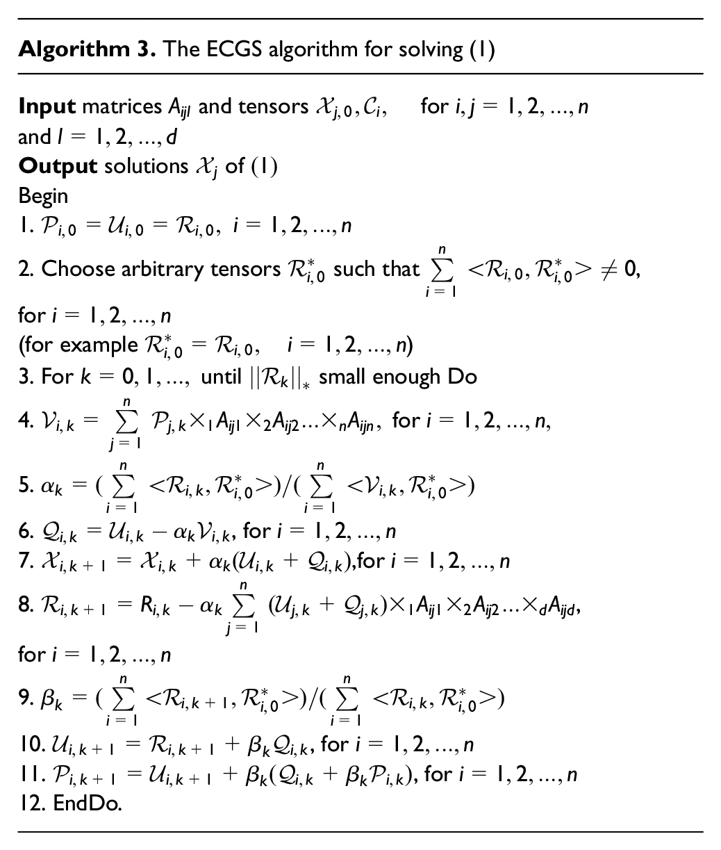
< v_{k}, r_{0}^{*} > = \sum_{i = 1}^{n} < V_{i, k}, R_{i, 0}^{*} >, < w_{k}, r_{0}^{*} > = \sum_{i = 1}^{n} < W_{i, k}, R_{i, 0}^{*} >,

< z_{k}, r_{0}^{*} > = \sum_{i = 1}^{n} < Z_{i, k}, R_{i, 0}^{*} > .

From the above discussion and based on Algorithm 1, we can describe the ECGS algorithm for solving (1) as follows.

Some important results concerning the ECGS algorithm are stated in the following theorem.

Theorem 3: The following properties hold.

(i) $\sum_{i = 1}^{n} < Q_{i, k}, R_{i, 0}^{*} > = 0 .$

(ii) $\sum_{i = 1}^{n} < U_{i, k + 1}, R_{i, 0}^{*} > = 0, \sum_{i = 1}^{n} < P_{i, k + 1}, R_{i, 0}^{*} > = 0 .$

(iii) $R_{i, k + 1} = C_{i} - \sum_{j = 1}^{n} X_{j, k + 1} \times_{1} A_{ij 1} \times_{2} A_{ij 2} . . . \times_{d} A_{ijd}, i = 1, 2, . . ., n .$

Proof:

$i$ . The proof is by induction on $k$ . For $k = 0$ ,

\begin{matrix} \sum_{i = 1}^{n} < Q_{i, 0}, R_{i, 0}^{*} > = \sum_{i = 1}^{n} < U_{i, 0} - α_{0} V_{i, 0}, R_{i, 0}^{*} > \\ = \sum_{i = 1}^{n} < U_{i, 0}, R_{i, 0}^{*} > - α_{0} \sum_{i = 1}^{n} < V_{i, 0}, R_{i, 0}^{*} > \\ = 0 . \end{matrix}

The last equation comes from line 1 of Algorithm 3 that implies $U_{i, 0} = R_{i, 0}$ and by definition of $α_{0}$ .

Algorithm 3. The ECGS algorithm for solving (1)
Input matrices $A_{ijl}$ and tensors $X_{j, 0}, C_{i},$ for $i, j = 1, 2, . . ., n$ and $l = 1, 2, . . ., d$ Output solutions $X_{j}$ of $(1)$ Begin 1. $P_{i, 0} = U_{i, 0} = R_{i, 0}, i = 1, 2, . . ., n$ 2. Choose arbitrary tensors $R_{i, 0}^{}$ such that $\sum_{i = 1}^{n} < R_{i, 0}, R_{i, 0}^{} > \neq 0$ , for $i = 1, 2, . . ., n$ (for example $R_{i, 0}^{} = R_{i, 0}, i = 1, 2, . . ., n$ ) 3. For $k = 0, 1, . . .,$ until $\| \| R_{k} \| \|_{}$ small enough Do 4. $V_{i, k} = \sum_{j = 1}^{n} P_{j, k} \times_{1} A_{ij 1} \times_{2} A_{ij 2} . . . \times_{n} A_{ijn},$ for $i = 1, 2, . . ., n,$ 5. $α_{k} = (\sum_{i = 1}^{n} < R_{i, k}, R_{i, 0}^{} >) / (\sum_{i = 1}^{n} < V_{i, k}, R_{i, 0}^{} >)$ 6. $Q_{i, k} = U_{i, k} - α_{k} V_{i, k}$ , for $i = 1, 2, . . ., n$ 7. $X_{i, k + 1} = X_{i, k} + α_{k} (U_{i, k} + Q_{i, k})$ ,for $i = 1, 2, . . ., n$ 8. $R_{i, k + 1} = R_{i, k} - α_{k} \sum_{j = 1}^{n} (U_{j, k} + Q_{j, k}) \times_{1} A_{ij 1} \times_{2} A_{ij 2} . . . \times_{d} A_{ijd}$ , for $i = 1, 2, . . ., n$ 9. $β_{k} = (\sum_{i = 1}^{n} < R_{i, k + 1}, R_{i, 0}^{} >) / (\sum_{i = 1}^{n} < R_{i, k}, R_{i, 0}^{} >)$ 10. $U_{i, k + 1} = R_{i, k + 1} + β_{k} Q_{i, k}$ , for $i = 1, 2, . . ., n$ 11. $P_{i, k + 1} = U_{i, k + 1} + β_{k} (Q_{i, k} + β_{k} P_{i, k})$ , for $i = 1, 2, . . ., n$ 12. EndDo.

Algorithm 3. The ECGS algorithm for solving (1)

Input matrices

A_{ijl}

and tensors

X_{j, 0}, C_{i},

for

i, j = 1, 2, . . ., n

and

l = 1, 2, . . ., d

Output solutions

X_{j}

(1)

Begin
1.

P_{i, 0} = U_{i, 0} = R_{i, 0}, i = 1, 2, . . ., n

2. Choose arbitrary tensors

R_{i, 0}^{*}

such that

\sum_{i = 1}^{n} < R_{i, 0}, R_{i, 0}^{*} > \neq 0

, for

i = 1, 2, . . ., n

(for example

R_{i, 0}^{*} = R_{i, 0}, i = 1, 2, . . ., n

)
3. For

k = 0, 1, . . .,

until

| | R_{k} | |_{*}

small enough Do
4.

V_{i, k} = \sum_{j = 1}^{n} P_{j, k} \times_{1} A_{ij 1} \times_{2} A_{ij 2} . . . \times_{n} A_{ijn},

for

i = 1, 2, . . ., n,

α_{k} = (\sum_{i = 1}^{n} < R_{i, k}, R_{i, 0}^{*} >) / (\sum_{i = 1}^{n} < V_{i, k}, R_{i, 0}^{*} >)

Q_{i, k} = U_{i, k} - α_{k} V_{i, k}

, for

i = 1, 2, . . ., n

X_{i, k + 1} = X_{i, k} + α_{k} (U_{i, k} + Q_{i, k})

,for

i = 1, 2, . . ., n

R_{i, k + 1} = R_{i, k} - α_{k} \sum_{j = 1}^{n} (U_{j, k} + Q_{j, k}) \times_{1} A_{ij 1} \times_{2} A_{ij 2} . . . \times_{d} A_{ijd}

, for

i = 1, 2, . . ., n

β_{k} = (\sum_{i = 1}^{n} < R_{i, k + 1}, R_{i, 0}^{*} >) / (\sum_{i = 1}^{n} < R_{i, k}, R_{i, 0}^{*} >)

10.

U_{i, k + 1} = R_{i, k + 1} + β_{k} Q_{i, k}

, for

i = 1, 2, . . ., n

11.

P_{i, k + 1} = U_{i, k + 1} + β_{k} (Q_{i, k} + β_{k} P_{i, k})

, for

i = 1, 2, . . ., n

12. EndDo.

Suppose that $i$ is true for $k = l - 1 > 0$ . For $k = l$

\begin{matrix} \sum_{i = 1}^{n} < Q_{i, l}, R_{i, 0}^{*} > = \sum_{i = 1}^{n} < U_{i, l} - α_{k} V_{i, l}, R_{i, 0}^{*} > \\ = \sum_{i = 1}^{n} < U_{i, l}, R_{i, 0}^{*} > - α_{l} \sum_{i = 1}^{n} < V_{i, l}, R_{i, 0}^{*} > \\ = \sum_{i = 1}^{n} < R_{i, l}, R_{i, 0}^{*} > - α_{l} \sum_{i = 1}^{n} < V_{i, l}, R_{i, 0}^{*} > \\ + β_{l - 1} \sum_{i = 1}^{n} < Q_{i, l - 1}, R_{i, 0}^{*} > \\ = \sum_{i = 1}^{n} < R_{i, l}, R_{i, 0}^{*} > - α_{l} \sum_{i = 1}^{n} < V_{i, l}, R_{i, 0}^{*} > \\ = 0 . \end{matrix}

The last two equations come form induction assumption that implies $\sum_{i = 1}^{n} < Q_{i, l - 1}, R_{i, 0}^{*} > = 0$ and the definition of $α_{l}$ .

By the same discussion, combining the ‘ $vec$ ‘ operator and the inherent properties of common CGS and this fact that the coefficient iterates $α_{k}$ and $β_{k}$ are derived based on their counterparts in Bi-CG for updating the residual tensors and the search direction tensors, the proof of relations $ii$ and $iii$ is easy. ■

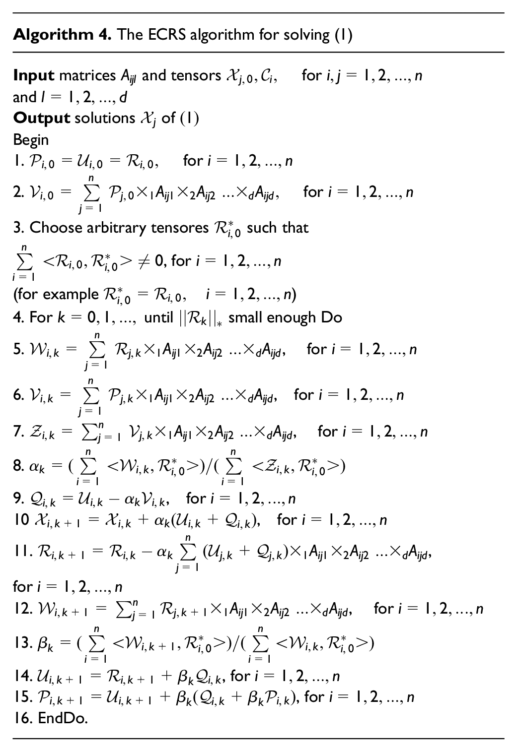
Based on Algorithm 2, we can describe the ECRS algorithm for solving $(1)$ as follows.

The next theorem lists a number of properties regarding the iterates in the above algorithm.

Theorem 4: The following properties hold

(i) $\sum_{i = 1}^{n} < Q_{i, k} \times_{1} A_{ij 1} \times_{2} A_{ij 2} . . . \times_{d} A_{ijd}, R_{i, 0}^{*} > = 0$ for $j = 1, 2, . . ., n$ .

(ii) $\sum_{i = 1}^{n} < U_{i, k + 1} \times_{1} A_{ij 1} \times_{2} A_{ij 2} . . . \times_{d} A_{ijd}, R_{i, 0}^{*} > = 0$ for $j = 1, 2, . . ., n$ .

(iii) $\sum_{i = 1}^{n} < P_{i, k + 1} \times_{1} A_{ij 1} \times_{2} A_{ij 2} . . . \times_{d} A_{ijd}, R_{i, 0}^{*} > = 0$ for $j = 1, 2, . . ., n$ .

(iv) $R_{i, k + 1} = C_{i} - \sum_{j = 1}^{n} X_{j, k + 1} \times_{1} A_{ij 1} \times_{2} A_{ij 2} . . . \times_{d} A_{ijd}$ , $i = 1, 2, . . ., n$ .

Proof:

$i$ . The proof is by induction on $k$ . For $k = 0$

\begin{matrix} \sum_{i = 1}^{n} < Q_{i, 0} \times_{1} A_{ij 1} \times_{2} A_{ij 2} . . . \times_{d} A_{ijd}, R_{i, 0}^{*} > \\ = \sum_{i = 1}^{n} < U_{i, 0} \times_{1} A_{ij 1} \times_{2} A_{ij 2} . . . \times_{d} A_{ijd} - α_{0} V_{i, 0} \times_{1} \\ A_{ij 1} \times_{2} A_{ij 2} . . . \times_{d} A_{ijd}, R_{i, 0}^{*} > \\ = \sum_{i = 1}^{n} < U_{i, 0} \times_{1} A_{ij 1} \times_{2} A_{ij 2} . . . \times_{d} A_{ijd}, R_{i, 0}^{*} > \\ - α_{0} \sum_{i = 1}^{n} < V_{i, 0} \times_{1} A_{ij 1} \times_{2} A_{ij 2} . . . \times_{d} A_{ijd}, R_{i, 0}^{*} > \\ = 0 . \end{matrix}

The last equation comes from line 1 of Algorithm 4 that implies $U_{i, 0} = R_{i, 0}$ and the definition of $α_{0}$ .

Algorithm 4. The ECRS algorithm for solving (1)
Input matrices $A_{ijl}$ and tensors $X_{j, 0}, C_{i},$ for $i, j = 1, 2, . . ., n$ and $l = 1, 2, . . ., d$ Output solutions $X_{j}$ of $(1)$ Begin 1. $P_{i, 0} = U_{i, 0} = R_{i, 0},$ for $i = 1, 2, . . ., n$ 2. $V_{i, 0} = \sum_{j = 1}^{n} P_{j, 0} \times_{1} A_{ij 1} \times_{2} A_{ij 2} . . . \times_{d} A_{ijd},$ for $i = 1, 2, . . ., n$ 3. Choose arbitrary tensores $R_{i, 0}^{}$ such that $\sum_{i = 1}^{n} < R_{i, 0}, R_{i, 0}^{} > \neq 0$ , for $i = 1, 2, . . ., n$ (for example $R_{i, 0}^{} = R_{i, 0}, i = 1, 2, . . ., n$ ) 4. For $k = 0, 1, . . .,$ until $\| \| R_{k} \| \|_{}$ small enough Do 5. $W_{i, k} = \sum_{j = 1}^{n} R_{j, k} \times_{1} A_{ij 1} \times_{2} A_{ij 2} . . . \times_{d} A_{ijd}$ , for $i = 1, 2, . . ., n$ 6. $V_{i, k} = \sum_{j = 1}^{n} P_{j, k} \times_{1} A_{ij 1} \times_{2} A_{ij 2} . . . \times_{d} A_{ijd}$ , for $i = 1, 2, . . ., n$ 7. $Z_{i, k} = \sum_{j = 1}^{n} V_{j, k} \times_{1} A_{ij 1} \times_{2} A_{ij 2} . . . \times_{d} A_{ijd}$ , for $i = 1, 2, . . ., n$ 8. $α_{k} = (\sum_{i = 1}^{n} < W_{i, k}, R_{i, 0}^{} >) / (\sum_{i = 1}^{n} < Z_{i, k}, R_{i, 0}^{} >)$ 9. $Q_{i, k} = U_{i, k} - α_{k} V_{i, k}$ , for $i = 1, 2, . . ., n$ 10 $X_{i, k + 1} = X_{i, k} + α_{k} (U_{i, k} + Q_{i, k})$ , for $i = 1, 2, . . ., n$ 11. $R_{i, k + 1} = R_{i, k} - α_{k} \sum_{j = 1}^{n} (U_{j, k} + Q_{j, k}) \times_{1} A_{ij 1} \times_{2} A_{ij 2} . . . \times_{d} A_{ijd}$ , for $i = 1, 2, . . ., n$ 12. $W_{i, k + 1} = \sum_{j = 1}^{n} R_{j, k + 1} \times_{1} A_{ij 1} \times_{2} A_{ij 2} . . . \times_{d} A_{ijd}$ , for $i = 1, 2, . . ., n$ 13. $β_{k} = (\sum_{i = 1}^{n} < W_{i, k + 1}, R_{i, 0}^{} >) / (\sum_{i = 1}^{n} < W_{i, k}, R_{i, 0}^{} >)$ 14. $U_{i, k + 1} = R_{i, k + 1} + β_{k} Q_{i, k}$ , for $i = 1, 2, . . ., n$ 15. $P_{i, k + 1} = U_{i, k + 1} + β_{k} (Q_{i, k} + β_{k} P_{i, k})$ , for $i = 1, 2, . . ., n$ 16. EndDo.

Algorithm 4. The ECRS algorithm for solving (1)

Input matrices

A_{ijl}

and tensors

X_{j, 0}, C_{i},

for

i, j = 1, 2, . . ., n

and

l = 1, 2, . . ., d

Output solutions

X_{j}

(1)

Begin
1.

P_{i, 0} = U_{i, 0} = R_{i, 0},

for

i = 1, 2, . . ., n

V_{i, 0} = \sum_{j = 1}^{n} P_{j, 0} \times_{1} A_{ij 1} \times_{2} A_{ij 2} . . . \times_{d} A_{ijd},

for

i = 1, 2, . . ., n

3. Choose arbitrary tensores

R_{i, 0}^{*}

such that

\sum_{i = 1}^{n} < R_{i, 0}, R_{i, 0}^{*} > \neq 0

, for

i = 1, 2, . . ., n

(for example

R_{i, 0}^{*} = R_{i, 0}, i = 1, 2, . . ., n

)
4. For

k = 0, 1, . . .,

until

| | R_{k} | |_{*}

small enough Do
5.

W_{i, k} = \sum_{j = 1}^{n} R_{j, k} \times_{1} A_{ij 1} \times_{2} A_{ij 2} . . . \times_{d} A_{ijd}

, for

i = 1, 2, . . ., n

V_{i, k} = \sum_{j = 1}^{n} P_{j, k} \times_{1} A_{ij 1} \times_{2} A_{ij 2} . . . \times_{d} A_{ijd}

, for

i = 1, 2, . . ., n

Z_{i, k} = \sum_{j = 1}^{n} V_{j, k} \times_{1} A_{ij 1} \times_{2} A_{ij 2} . . . \times_{d} A_{ijd}

, for

i = 1, 2, . . ., n

α_{k} = (\sum_{i = 1}^{n} < W_{i, k}, R_{i, 0}^{*} >) / (\sum_{i = 1}^{n} < Z_{i, k}, R_{i, 0}^{*} >)

Q_{i, k} = U_{i, k} - α_{k} V_{i, k}

, for

i = 1, 2, . . ., n

X_{i, k + 1} = X_{i, k} + α_{k} (U_{i, k} + Q_{i, k})

, for

i = 1, 2, . . ., n

11.

R_{i, k + 1} = R_{i, k} - α_{k} \sum_{j = 1}^{n} (U_{j, k} + Q_{j, k}) \times_{1} A_{ij 1} \times_{2} A_{ij 2} . . . \times_{d} A_{ijd}

, for

i = 1, 2, . . ., n

12.

W_{i, k + 1} = \sum_{j = 1}^{n} R_{j, k + 1} \times_{1} A_{ij 1} \times_{2} A_{ij 2} . . . \times_{d} A_{ijd}

, for

i = 1, 2, . . ., n

13.

β_{k} = (\sum_{i = 1}^{n} < W_{i, k + 1}, R_{i, 0}^{*} >) / (\sum_{i = 1}^{n} < W_{i, k}, R_{i, 0}^{*} >)

14.

U_{i, k + 1} = R_{i, k + 1} + β_{k} Q_{i, k}

, for

i = 1, 2, . . ., n

15.

P_{i, k + 1} = U_{i, k + 1} + β_{k} (Q_{i, k} + β_{k} P_{i, k})

, for

i = 1, 2, . . ., n

16. EndDo.

Suppose that $i$ is true for $k = l - 1 > 0$ . For $k = l$

\begin{matrix} \sum_{i = 1}^{n} < Q_{i, l} \times_{1} A_{ij 1} \times_{2} A_{ij 2} . . . \times_{d} A_{ijd}, R_{i, 0}^{*} > \\ = \sum_{i = 1}^{n} < U_{i, l} \times_{1} A_{ij 1} \times_{2} A_{ij 2} . . . \times_{d} A_{ijd} - α_{l} V_{i, l} \times_{1} \\ A_{ij 1} \times_{2} A_{ij 2} . . . \times_{d} A_{ijd}, R_{i, 0}^{*} > \\ = \sum_{i = 1}^{n} < R_{i, l} \times_{1} A_{ij 1} \times_{2} A_{ij 2} . . . \times_{d} A_{ijd}, R_{i, 0}^{*} > \\ - α_{l} \sum_{i = 1}^{n} < V_{i, l} \times_{1} A_{ij 1} \times_{2} A_{ij 2} . . . \times_{d} A_{ijd}, R_{i, 0}^{*} > \\ + β_{l - 1} \sum_{i = 1}^{n} < Q_{i, l - 1} \times_{1} A_{ij 1} \times_{2} A_{ij 2} . . . \times_{d} A_{ijd}, R_{i, 0}^{*} > \\ = \sum_{i = 1}^{n} < R_{i, l} \times_{1} A_{ij 1} \times_{2} A_{ij 2} . . . \times_{d} A_{ijd}, R_{i, 0}^{*} > \\ - α_{l} \sum_{i = 1}^{n} < V_{i, l} \times_{1} A_{ij 1} \times_{2} A_{ij 2} . . . \times_{d} A_{ijd}, R_{i, 0}^{*} > \\ = 0 . \end{matrix}

The last two equations come form induction assumption that implies

$\sum_{i = 1}^{n} < Q_{i, l - 1} \times_{1} A_{ij 1} \times_{2} A_{ij 2} . . . \times_{d} A_{ijd}, R_{i, 0}^{*} > = 0$ and the definition of $α_{l}$ .

By the same discussion, combining the ‘ $vec$ ‘ operator and the inherent properties of common CRS and this fact that the coefficient iterates $α_{k}$ and $β_{k}$ are derived based on their counterparts in Bi-CR for updating the residual tensors and the search direction tensors, the proof of relations $ii, iii$ and $iv$ is obtained.

Numerical examples

In this section, we give some numerical examples to show the effectiveness of the proposed algorithms. For this purpose we compare the ECGS and ECRS algorithms with Bi-CG, Bi-CR, LSQR, CGLS, GI, all in tensor forms that we have done only their codes and avoided here the related algorithms, and GLS-BTF (Karimi and Dehghan, 2017) algorithms. All examples were carried out in double precision with a MATLAB code, while the computer specifications are Microsoft Windows XP Intel(R), Core(TM)i7-7500U, CPU 2.70 GHz, with 8 GB of RAM.

In all of the following examples we choose initial tensors $X_{j, 0} = O, j = 1, 2, . . . n$ .

Example 1: (Karimi and Dehghan, 2017; Xu and Wang, 2019). First, we consider the equation

- ν Δ u + c^{T} \nabla u = f, in Ω = [0, 1] \times [0, 1] \times [0, 1],

u = 0, on \partial Ω .

A standard finite difference discretization on equidistant nodes (mesh-size $h = 1 / (n + 1)$ ), combined with a second order convergent scheme (Fromm’s scheme) for the term $c^{T} \nabla u$ , leads to the linear system $Ax = b$ where $A = I_{n} \otimes I_{n} \otimes A_{1} + I_{n} \otimes A_{2} \otimes I_{n} + A_{3} \otimes I_{n} \otimes I_{n},$ and

A_{i} = \frac{ν}{h^{2}} (\begin{matrix} - 2 & 1 \\ 1 & - 2 & 1 \\ ⋱ & ⋱ & ⋱ \\ 1 & - 2 & 1 \\ 1 & - 2 \end{matrix}) + \frac{c_{i}}{4 h} (\begin{matrix} - 3 & 5 & - 1 \\ - 1 & - 3 & 5 & ⋱ \\ ⋱ & ⋱ & ⋱ & - 1 \\ - 1 & - 3 & 5 \\ - 1 & - 3 \end{matrix}), i = 1, 2, 3 .

The corresponding tensor equation is $X \times_{1} A_{1} + X \times_{2} A_{2} + X \times_{3} A_{3} = C,$ which can be regarded as the Sylvester tensor equation $(3)$ . For

\begin{matrix} (a) . ν = 1, c_{1} = 0.1, c_{2} = 0.2, c_{3} = 0.3, n = 25 \\ (b) . ν = 3, c_{1} = 1, c_{2} = 2, c_{3} = 3, n = 50, \\ (c) . ν = 5, c_{1} = 5, c_{2} = 5, c_{3} = 5, n = 75, \\ (d) . ν = 2, c_{1} = 5, c_{2} = 10, c_{3} = 15, n = 100, \end{matrix}

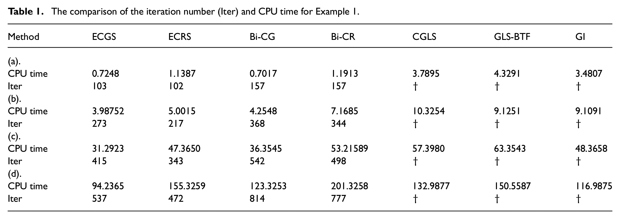
we apply the mentioned algorithms to compute the sequence ${X_{j}}$ . For simplicity, we construct the right-hand side tensor $C$ such that the exact solution would be a tensor where all of its elements are equal to one. The numerical results are presented in the Table 1, where the stopping criterion is $\frac{| | R_{j} {| |}_{*}}{| | R_{0} {| |}_{*}} < 10^{- 10}$ . We use † to indicate that there was no convergence up to 1000 iterations.

Table 1.

The comparison of the iteration number (Iter) and CPU time for Example 1.

Method	ECGS	ECRS	Bi-CG	Bi-CR	CGLS	GLS-BTF	GI
(a).
CPU time	0.7248	1.1387	0.7017	1.1913	3.7895	4.3291	3.4807
Iter	103	102	157	157	†	†	†
(b).
CPU time	3.98752	5.0015	4.2548	7.1685	10.3254	9.1251	9.1091
Iter	273	217	368	344	†	†	†
(c).
CPU time	31.2923	47.3650	36.3545	53.21589	57.3980	63.3543	48.3658
Iter	415	343	542	498	†	†	†
(d).
CPU time	94.2365	155.3259	123.3253	201.3258	132.9877	150.5587	116.9875
Iter	537	472	814	777	†	†	†

The numerical results in Table 1 show the superiority of ECGS and ECRS over other methods.

Example 2: In this example, we consider the tensor equation (7) with parameters

A_{1} = triu (rand (m), 1) + i \times diag (2.75 + diag (rand (m))),

A_{2} = tril (rand (n), 1) - 2 i \times diag (1.5 + diag (rand (n))),

A_{3} = triu (rand (l), l) + diag (1.5 + diag (rand (l))),

B_{1} = (triu (rand (m), 1) - diag (1.5 + diag (rand (m)))),

B_{2} = tril (rand (n), 1) - diag (2 + diag (rand (n))),

B_{3} = triu (rand (l), l) + i \times diag (2 + diag (rand (l))),

D_{1} = triu (rand (m), 1) + 3 i \times diag (1 + diag (rand (m))),

D_{2} = tril (rand (n), 1) - diag (1.5 + diag (rand (n))),

D_{3} = triu (rand (l), l) - i \times diag (1 + diag (rand (l))),

E_{1} = (triu (rand (m), 1) - diag (2 + diag (rand (m)))),

E_{2} = triu (rand (n), n) + diag (1.5 + diag (rand (n))),

E_{3} = (triu (rand (l), 1) - diag (1.5 + diag (rand (l)))) .

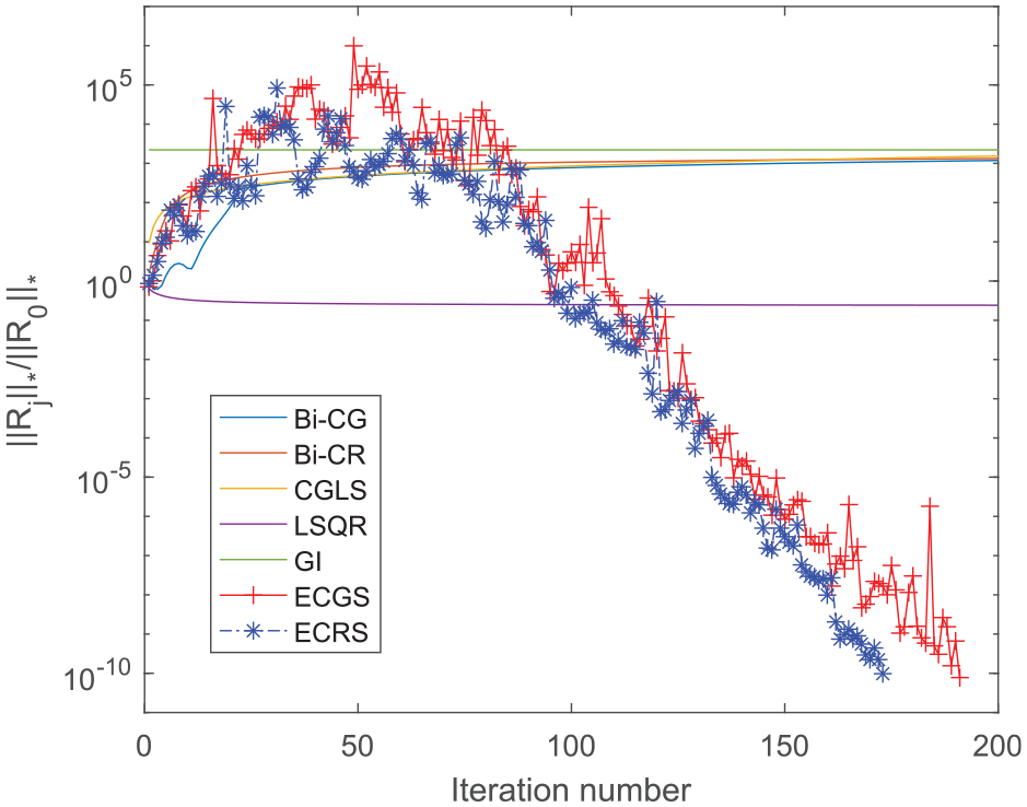
By choosing $C$ , $F$ such that the exact solution would be a tensors where all of their elements are equal to one and applying the mentioned algorithms for $m = 40$ , $n = 30$ and $l = 20$ , we compute ${X_{j}}$ and ${Y_{j}}$ . The convergence curves are shown in Figure 1, where the stopping criterion is $\frac{| | R_{j} {| |}_{*}}{| | R_{0} {| |}_{*}} < 10^{- 10} .$ As shown in Figure 1, the ECGS and ECRS algorithms have more superiority over other algorithms.

Example 3: (Xu and Wang, 2019). Consider the Stein tensor equation

X - X \times_{1} A_{1} \times_{2} A_{2} \times_{3} A_{3} = C,

with

\begin{matrix} A_{1} = tril (rand (m), 1) + i \times diag (1.5 + diag (rand (m))), \\ A_{2} = triu (rand (n), 1) - 2 i \times diag (2 + diag (rand (n))), \\ A_{3} = triu (rand (l), l) + diag (1.5 + diag (rand (l))), \\ C = i \times tenrand (m, n, l) . \end{matrix}

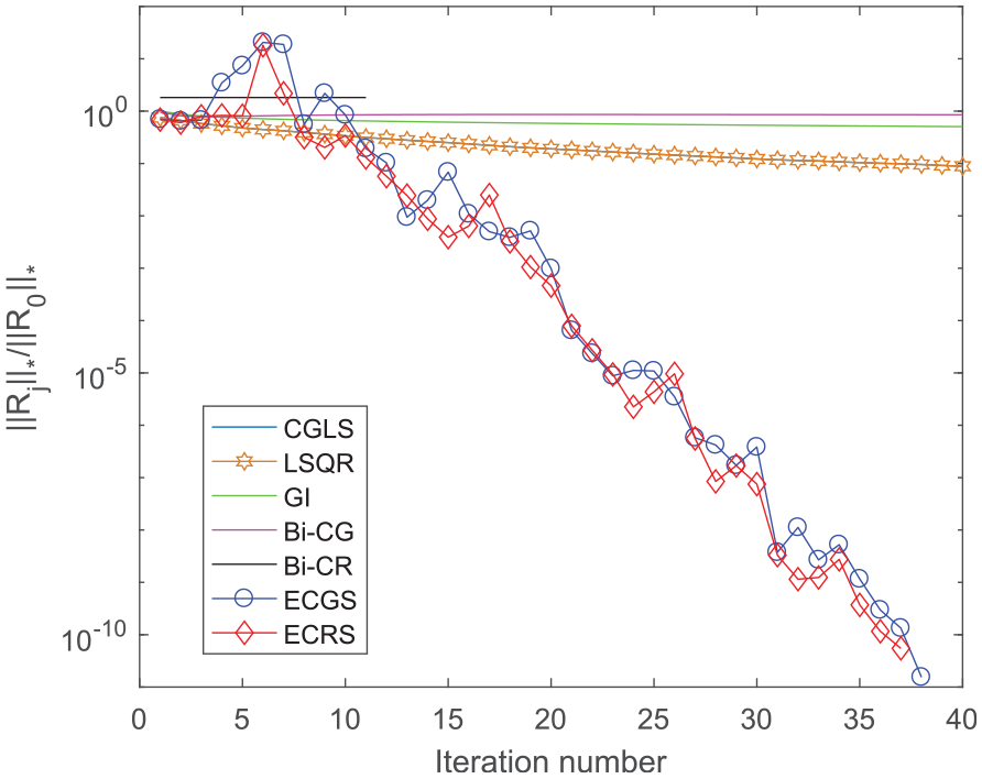
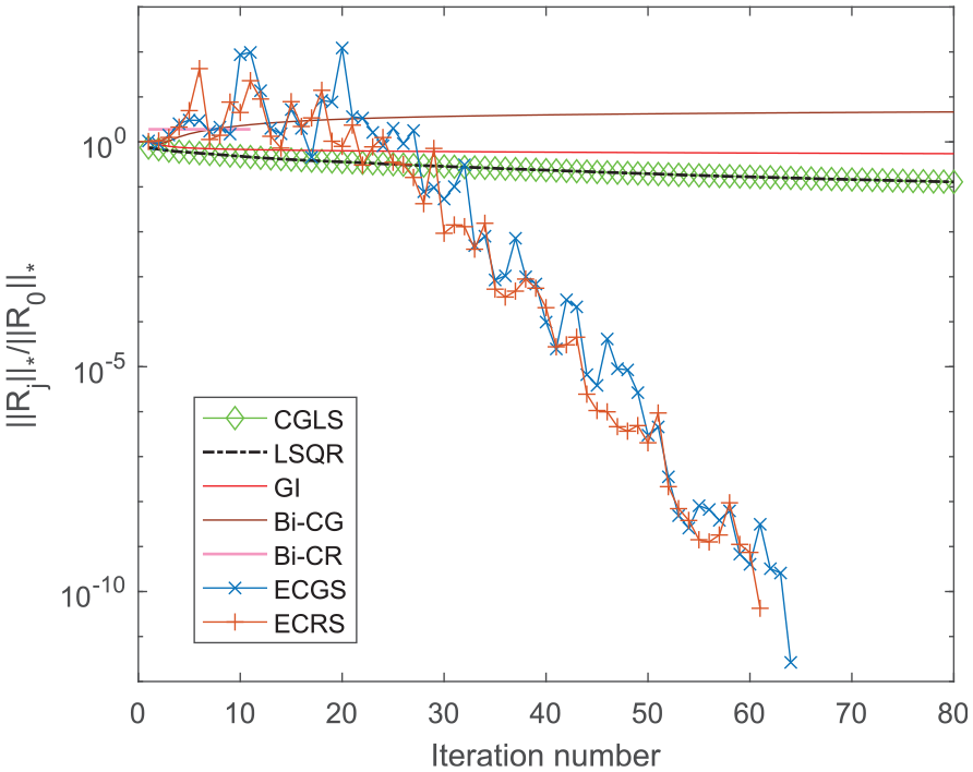
For (a). $m = 30, n = 20$ , $l = 10$ and (b). $m = 50, n = 40$ , $l = 30$ , we apply the mentioned algorithms to compute ${X_{j}}$ . The corresponding convergence histories are depicted in Figures 2 and 3, respectively.

Example 4: Finally, let us consider the generalized coupled Sylvester tensor equations

{\begin{matrix} X \times_{1} A_{1} \times_{2} A_{2} + Y \times_{1} B_{1} \times_{2} B_{2} + Z \times_{1} C_{1} \times_{2} C_{2} = D \\ X \times_{1} E_{1} \times_{2} E_{2} + Y \times_{1} F_{1} \times_{2} F_{2} + Z \times_{1} G_{1} \times_{2} G_{2} = H \\ X \times_{1} I_{1} \times_{2} I_{2} + Y \times_{1} J_{1} \times_{2} J_{2} + Z \times_{1} K_{1} \times_{2} K_{2} = L, \end{matrix}

with parameters

A_{1} = i \times triu (rand (m, m), 1) + diag (1.75 + diag (rand (m))), A_{2} = tril (rand (n, n), 1) + diag (1.5 + diag (rand (n)))

B_{1} = - triu (rand (m, m), 1) - i \times diag (1.5 + diag (rand (m))), B_{2} = tril (rand (n, n), 1) + diag (2 + diag (rand (n)))

C_{1} = triu (rand (m, m), 1) - 2 i \times diag (2 + diag (rand (m))), C_{2} = tril (rand (n, n), 1) + diag (1.5 + diag (rand (n)))

E_{1} = - i \times triu (rand (m, m), 1) - diag (2 + diag (rand (m))), E_{2} = triu (rand (n, n), n) + diag (1.5 + diag (rand (n)))

F_{1} = i \times triu (rand (m, m), 1) + diag (1.75 + diag (rand (m))), F_{2} = tril (rand (n, n), 1) + diag (1.5 + diag (rand (n)))

G_{1} = - triu (rand (m, m), 1) - i \times diag (1.5 + diag (rand (m))), G_{2} = tril (rand (n, n), 1) + diag (2 + diag (rand (n)))

I_{1} = triu (rand (m, m), 1) - 2 i \times diag (2 + diag (rand (m))), I 2 = tril (rand (n, n), 1) + diag (1.5 + diag (rand (n)))

J_{1} = - i \times triu (rand (m, m), 1) - diag (2 + diag (rand (m))))), J_{2} = triu (rand (n, n), n) + diag (1.5 + diag (rand (n)))

K_{1} = i \times triu (rand (m, m), 1) + diag (1.75 + diag (rand (m))), K_{2} = tril (rand (n, n), 1) + diag (1.5 + diag (rand (n)))

D = i \times tenrand (m, n, l), H = i \times tenrand (m, n, l), L = i \times tenrand (m, n, l) .

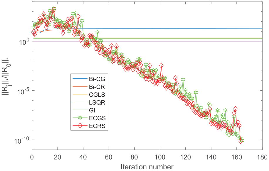
For $m = 40$ , $n = 30$ and $l = 20$ , by applying the mentioned algorithms we compute the sequences ${X_{j}}$ , ${Y_{j}}$ and ${Z_{j}}$ . The convergence curves are depicted in Figure 4, which shows the performance of the proposed algorithms.

Concluding remarks

In this paper, we have proposed the ECGS and ECRS methods for solving general coupled Sylvester tensor equations (1). These methods are base on tensor format. In contrast with the common CGS and CRS methods for solving matricization form of (1), the ECGS and ECRS methods need the less flops and storage. Inspired by the properties of CGS and CRS, we have presented some properties of the new methods. Our numerical results have shown that the proposed methods perform much better than others.

Footnotes

Acknowledgements

The authors would like to thank the anonymous referees for their comments and suggestions, which helped to considerably improve the manuscript.

Declaration of conflicting interests

The author(s) declared no potential conflicts of interest with respect to the research, authorship, and/or publication of this article.

Funding

The author(s) received no financial support for the research, authorship, and/or publication of this article.

ORCID iDs

Eisa Khosravi Dehdezi

Saeed Karimi

References

Bai

Golub

(2003) Hermitian and skew-hermitian splitting methods for non-hermitian positive definite linear systems. SIAM Journal on Matrix Analysis and Applications 24(3): 603–626.

Beik

FPA

Ahmadi Asl

(2015) Residual norm steepest descent based iterative algorithms for Sylvester tensor equations. Journal of Mathematical Modeling 2(2): 115–131.

Beik

FPA

Saberi Movahed

Ahmadi Asl

(2016) On the Krylov subspace methods based on tensor format for positive definite Sylvester tensor equations. Numerical Linear Algebra with Applications 23(3): 444–466.

Brazell

Navasca

, et al. (2013) Solving multilinear systems via tensor inversion. SIAM Journal on Matrix Analysis and Applications 34(2): 542–570.

Chen

Yin

Huang

G-X

(2012) An iterative algorithm for the generalized reflexive solution of the matrix equations AXB = E, CXD = F. Journal of Applied Mathematics 2012(3): 1–20.

Chen

(2012) A projection method and Kronecker product preconditioner for solving Sylvester tensor equations. Science China Mathematics 55(6): 1281–1292.

Ding

Chen

(2005a) Gradient based iterative algorithms for solving a class of matrix equations. IEEE Transactions on Automatic Control 50(8): 1216–1221.

Ding

Chen

(2005b) Iterative least squares solutions of coupled Sylvester matrix equations. Systems and Control Letters 54(2): 95–107.

Grasedyck

(2004) Existence and computation of low Kronecker-rank approximations for large linear systems of tensor product structure. Computing 72(3–4): 247–265.

10.

Golub

Nash

Van Loan

(1978) A Hessenberg-Schur method for the problem AX + XB = C. IEEE Transactions on Automatic Control 24(6): 909–913.

11.

Kagström

Westin

(1989) Generalized Schur methods with condition estimators for solving the generalized Sylvester equation. IEEE Transactions on Automatic Control 34(7): 745–751.

12.

Karimi

Dehghan

(2018) Global least squares method based on tensor form to solve linear systems in Kronecker format. Transactions of the Institute of Measurement and Control 40(7): 2378–2386.

13.

Kolda

(2006) Multilinear operators for higher-order decompositions. Tech. Report SAND2006–2081.

14.

Kolda

Bader

(2009) Tensor decompositions and applications. SIAM Review 51(3): 455–500.

15.

Sun

Y-S

Zhang

D-W

(2009) Chebyshev collocation spectral methods for coupled radiation and conduction in a concentric spherical participating medium. ASME Journal of Heat Transfer 131(6): 062701 (9 pages).

16.

Tian

Sun

, et al. (2010) Schur-decomposition for 3D matrix equations and its application in solving radiative discrete ordinates equations discretized by Chebyshev collocation spectral method. Journal of Computational Physics 229(4): 1198–1212.

17.

Paige

Saunders

(1982) LSQR: an algorithm for sparse linear equations and sparse least squares. ACM Transactions on Mathematical Software 8(1): 43–71.

18.

Saad

(2003) Iterative Methods for Sparse Linear Systems, 2nd Edn. Philadelphia: SIAM.

19.

Shi

Wei

Ling

(2013) Backward error and perturbation bounds for high order Sylvester tensor equation. Linear and Multilinear Algebra 61(10): 1436–1446.

20.

Sonneveld

(1989) CGS, a fast Lanczos-type solver for nonsymmetric linear systems. SIAM Journal on Scientific and Statistical Computing 10(1): 36–52.

21.

Sun

Zheng

Wei

(2016) Moore penrose inverse of tensors via Einstein product. Linear and Multilinear Algebra 64(4): 686–698.

22.

Wanga

Q-W

(2019) Extending Bi-CG and Bi-CR methods to solve the Stein tensor equation. Computers and Mathematics with Applications 77(12): 3117–3127.